Modeling COVID-19 for Lifting Non-Pharmaceutical Interventions

, ,
and
The MITRE Corporation, United States
Journal of Artificial
Societies and Social Simulation 24 (2) 9
<https://www.jasss.org/24/2/9.html>
DOI: 10.18564/jasss.4585
Received: 09-Nov-2020 Accepted: 25-Mar-2021 Published: 31-Mar-2021
Abstract
As a result of the COVID-19 worldwide pandemic, the United States instituted various non-pharmaceutical interventions (NPIs) in an effort to slow the spread of the disease. Although necessary for public safety, these NPIs can also have deleterious effects on the economy of a nation. State and federal leaders need tools that provide insight into which combination of NPIs will have the greatest impact on slowing the disease and at what point in time it is reasonably safe to start lifting these restrictions to everyday life. In the present work, we outline a modeling process that incorporates the parameters of the disease, the effects of NPIs, and the characteristics of individual communities to offer insight into when and to what degree certain NPIs should be instituted or lifted based on the progression of a given outbreak of COVID-19. We apply the model to the 24 county-equivalents of Maryland and illustrate that different NPI strategies can be employed in different parts of the state. Our objective is to outline a modeling process that combines the critical disease factors and factors relevant to decision-makers who must balance the health of the population with the health of the economy.Introduction
In December of 2019, a cluster of pneumonia cases of unknown origin were identified in Wuhan, China. An investigation into the cases commenced in early January 2020 that led to the discovery of a novel coronavirus now designated SARS-CoV-2. The virus causes an infectious disease now known as Coronavirus Disease 2019 or COVID-19. Common symptoms of COVID-19 include shortness of breath, fever, dry cough, fatigue, and respiratory distress. On March 11th, 2020, the World Health Organization declared a global pandemic. As of this writing, global deaths exceed 2.3 million according to Johns Hopkins University (Johns Hopkins University 2020) and COVID-19 cases have been confirmed in 192 countries and regions around the world.
Prior to November 2020, there was no approved vaccine effective against COVID-19 (Rothan & Byrareddy 2020). Treatment involves addressing the symptoms as the virus runs its course. Therefore, most countries have implemented NPIs in an effort to prevent the spread of COVID-19. These interventions usually involve restricting the movements of the population. The U.S. has employed school closures, shelter-in-place orders, business closures, limits on or banning of public gatherings, closing public spaces such as parks, and social distancing orders that require people to stay at least six feet from each other. In addition, a combination of testing and tracing anyone who came in contact with a positive case – referred to as contact tracing – and requiring them to self-quarantine for approximately 14 days is another tactic for limiting the spread.
The restrictions to daily life have driven the world into one of the largest recessions in history (Gopinath 2020). The Bureau of Economic Analysis reported that U.S. real Gross Domestic Product (GDP) contracted 31.4% in the second quarter and the U.S. unemployment rate rose from 3.6% in January 2020 to 14.7% in April 2020 (Analysis 2020; Labor & Statistics 2020). The economic recession creates an urgency to lift the NPIs and population restrictions that is in direct conflict with the desire to stop the spread of disease and keep the population healthy. State and federal leaders therefore need tools that can provide insight into the risk to populations of lifting NPIs before the disease is completely wiped out or a vaccine is developed. In response to this need and in keeping with the call to action from Squazzoni et al. (2020), we present an agent-based, social contact network driven approach to modeling how NPIs will impact the pandemic in a given region.
The dynamics of a pandemic are a function of the biological characteristics of the disease, the biologic response of those infected, and the behaviors of those in the region affected by the disease. In this way a pandemic is an emergent phenomenon of the social systems within which it is embedded (Epstein 2006; Galea et al. 2010). Emergent phenomena are a characteristic of complex systems (Cowan 1999; Mitchell 2009), and an efficient way to discover their future state is to simulate the dynamics (Buss et al. 1990) with an agent-based model (ABM) (Axtell 2000; Wilensky & Rand 2015). In these types of systems the interactions among agents are as important to the overall dynamics as the characteristics of the agents themselves. Indeed, empirical studies have shown that the same disease can exhibit heterogeneous transmission characteristics as it spreads to different communities (Meyers et al. 2005). This fact led researchers to look for ways to more realistically model the contact structure of a given population (Bansal et al. 2007). Bansal et al. conclude that homogeneous mixing is an over-simplified assumption and that some degree of heterogeneity in the contact network is necessary to accurately model the spread of a disease. However, community structure itself is dynamic and changes naturally or forcibly over time, such as in response to changing environmental conditions. Thus, incorporating heterogeneous mixing by modeling a contact network is still a simplified assumption if that network remains static within the model.
NPIs are designed to deliberately reduce physical contact among the population, thereby changing the contact structure. A strict reductionist approach to this problem will only provide partial insights into the system dynamics. Further, as pointed out by Manzo (2020), other features of the social contact network can impact the spread of disease. He notes specifically the relationships between the degree distribution, the clustering of ego-centered networks, and the high reachability of global networks impact the probability of contact between members of otherwise distant social circles. These features not only contribute to the spread of diseases, but they can also inform targeted interventions that more effectively deter widespread pandemics. Other authors, notably, Block et al. (2020) and Nishi et al. (2020), have noted that intervention strategies should take the network structure into account. Manzo & Rijt (2020) show specifically that targeting hubs in the contact network can improve containment of disease.
The challenge for decision-makers faced with a deadly pandemic is therefore to estimate the initial contact structure of their community and then determine how that structure might change when different NPIs are implemented. In the current work, we establish a procedure for inferring the degree distribution of a given county in the U.S. from Census data (Census 2020). This provides a pre-pandemic community structure. We then constructed an agent-based model (ABM) that incorporates the daily behavior of individuals in a given community, along with the constraints to that behavior imposed by NPIs. The ABM ingests the pre-pandemic community network inferred from Census data to drive heterogeneous social contact when no NPIs are implemented. The post-pandemic contact structure emerges as a function of compliance with NPIs and we are able to assess differences in the spread of disease as a function of both contact network degree distribution and the impact that a given set of NPIs has on the network structure. When NPIs are imposed on the agent population the underlying contact network is disrupted. The severity of the disruption is a function of which specific NPIs are used, the compliance of the agents, and the outcome of the random variables incorporated into the model logic.
To illustrate the utility of our approach we model the 24 county-equivalents of Maryland. We show that different strategies can have the same impact on disease progression depending on the contact structure of each county. The ABM combined with the inferred contact network structure allows decision-makers to determine which factors are most important in classifying the risk of large outbreaks in different regions and facilitates the customization of NPI strategies. In the sections that follow, we describe the algorithm for inferring contact structure and outline the architecture of the ABM. We then describe the design of experiments that addresses our hypothesis about NPI strategies. Finally, we present the key outcomes from the simulation experiment and we close with a brief discussion.
Materials and Methods
Inferring network structure
Newman (2002) showed that the degree distribution of the contact network of a society, along with the characteristics of the disease, determines the size of an outbreak in a given community. Meyers et al. (2005) demonstrated this result for the SARS outbreak of 2003, noting that outbreaks of SARS occurring nearly simultaneously in different parts of Canada had vastly different progressions. In order to have a practically useful model of disease progression, we must therefore estimate the degree distribution of the contact network of each community. Fortunately, the U.S. Census conducts an extensive annual survey known as the American Community Survey (ACS) (Census 2020). The ACS provides county level information on characteristics of the population such as households, household size, school enrollment, occupation, and age distribution. Meyers et al. (2005) outlined a process for taking comparable data (their study focused on Vancouver, Canada) and inferring a network structure based on a few simplifying assumptions. Here we design a similar algorithm using the ACS data to create county-level social contact networks that are likely to be representative of human-to-human contact before the outbreak of COVID-19 and the associated NPIs.
Meyers et al. (2005) assumed that individuals living in the same household would have physical contact with probability \(p_{h} = 1.0\). That is, every vertex in a household has an edge with every other vertex in the same household. Once the household subgraphs are created, the population is then assigned to schools based on their age group and school enrollment data, and workplaces based on occupation data. Individuals who attend the same school have a physical contact with probability \(p_{s}=0.3\) and those who work together have contact with probability \(p_{o}=0.03\). Finally, people have friends, go to restaurants and stores, and otherwise interact socially. These public contacts occur with probability \(p_{p}=0.003\) and can involve any two individuals in the community. These parameters were also taken from Meyers et al. (2005) and we found empirically that they work well for the counties we studied. The full algorithmic statement is shown in Figure 1, but the basic premise is straightforward. Using the necessary values from the ACS, the contact network for each county-equivalent is built incrementally as follows:
- Create a vector of vertices distributed according to the ACS age brackets
- Group the vertices into households according to the ACS data
- Assign edges between members of a household with probability \(p_h\)
- For each school level, assign edges between pairs of appropriate vertices with probability \(p_s\)
- For each occupation assign edges between pairs of appropriate vertices with probability \(p_o\)
- For all vertices assign edges between pairs with probability \(p_p\)
The Agent-based model
The ABM was built in the NetLogo multi-agent programmable modeling environment version 6.1.1 (Wilensky 1999). The basic model components are:
- the disease progression model
- the population of agents and their social contact structure
- the environment consisting of schools, homes, hospitals, workplaces, and public venues, and
- the logic of NPIs, testing, and contact tracing.
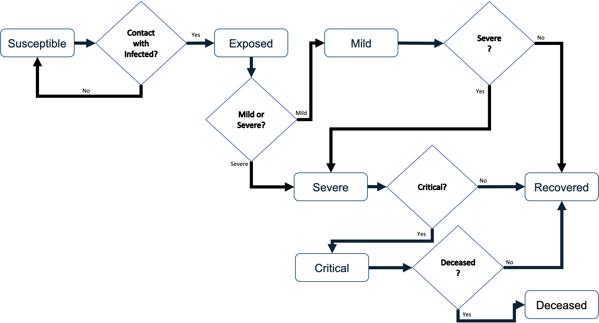
The disease progression model was designed to follow the dynamics of COVID-19 as they were understood as of March of 2020. Based on the classic Susceptible, Exposed, Infected, Recovered (SEIR) model, the agents move through discrete states as the virus runs its course. The disease states include Susceptible, Exposed, Mild, Severe, Critical, Deceased, and Recovered. When the model is initiated, most agents are instantiated as Susceptible except for a small number of user-specified number of agents who are initiated as Exposed in order to generate the outbreak. These few exposed agents progress to either Mild or Severe after the parameterized time duration of the Exposed state, at which point they can infect other agents with whom they come into contact.
The duration of each disease state is a parameter that can be overridden by the user, which facilitates flexibility and response to changes driven by emerging research in COVID-19 disease progression. The default dynamics are outlined in Table 1 (Lauer et al. 2020; Huang et al. 2020; CDC COVID-19 Response Team et al. 2020; Sanche et al. 2020; Eubank et al. 2020; Wang et al. 2020a; Wu and McGoogan 2020; Wang et al. 2020b ). We used a combination of published studies and pre-publication data on MedRxiv to establish the disease transmission parameters, but it should be noted that studies of COVID-19 are ongoing and these parameters should be updated at the time the model is being used for decision-making. For our purposes, these parameters worked well when fitting to the empirical data available at the time of our study.
| Time Period | Duration | Transition Probabilities | Value |
| Exposed Period | 5 days | From Exposed to Severe | 0.12 |
| Mild Period | 6 days | From Exposed to Mild | 0.88 |
| Severe Period | 4 days | From Mild to Severe | 0.40 |
| Critical Period (hospitalized) | 10 days | From Severe to Critical | 0.40 |
| Critical Period (at home) | 3 days | From Critical to Deceased | 0.60 or 1.0 at home |
The dynamics of COVID-19 progression are both time-based and stochastic. That is, different states of the disease have well-documented time frames, but the chance of an agent progressing through a mild or severe case is stochastic. When agents are co-located, there is some chance that the disease will be transferred from one agent to another. At each time step agents that are contagious (those in the Mild, Severe, or Critical states) will look for another agent on the same patch (small piece of the environment). If there is at least one other agent on the patch contagious agents will attempt to pass the virus to one other agent. Successful passing of the virus is a function of a user-specified probability of successfully getting the virus on the other agent, a user-specified mitigation probability, and the health status of the target agent (if they are already sick, they will not get sicker). The first two probability parameters allow the user to simulate situations such as wearing masks, maintaining social-distance, and hand-washing.
Once an agent becomes Exposed after five days they will move to either the Mild state (0.88 chance) or Severe state (0.12 chance). If the agent transitions to the Severe state, then after four days they will transition to either the Critical state (0.40 chance) or the Recovered state (0.60 chance). If on the other hand, the agent transitions to the Mild state from the Exposed state, after six days they will either transition to Severe state (0.40 chance) or the Recovered state (.60 chance). Once in the Recovered state agents are no longer able to contract the disease. Agents in the Critical state are assumed to need breathing assistance and significant medical support; therefore, if the agent is unable to go to the hospital within three days of becoming critical they will die with probability 1.0. Agents are contagious when they are in the Mild, Severe, or Critical states. The Mild state includes both symptomatic and asymptomatic agents and each agent has an attribute indicating which category they are in. It is assumed that agents in the Exposed state are not contagious. That is, the Exposed state represents an incubation period where the viral load in the agent is too low to infect others. This state is not the same as an asymptomatic state. Once agents progress to the Mild state they may be asymptomatic or symptomatic.
The next component of the ABM is the environment, which includes both physical spaces and the initial social contact structure of the population. The model is instantiated with the inferred contact network of a U.S. county scaled to be approximately 10,000 agents. These contact structures are generated using U.S. Census data and the algorithm described in the previous section. The size of the ABM environment is then adjusted to approximate the population density of the county in question. The physical space is created from the aforementioned networks. Agents are assigned to a school, work, public venue, and homes. The locations are then placed in the modeling environment. They can be mixed, as one might see in an urban area where individuals live, work, shop, and learn in close proximity or home locations can be more separated as one might see in rural or suburban counties.
The NPI component of the ABM is integrated into these physical locations and the agent behaviors. As the simulation runs, each agent spends one 12-hour time step at home and the next 12-hour time step at work, school, or a public venue as long as going to that venue is not prohibited by an NPI. The available NPIs include closing schools, closing work places, closing public venues, imposing social distancing requirements (i.e., stay home orders), and isolating individuals. Individual mitigation steps can also be modeled using the probabilities associated with disease transmission, as mentioned earlier.
The final model component is the logic of testing and contact tracing. There are two alternative testing strategies incorporated into the ABM; random selection of everyone not in the hospital, or targeted testing of a specific percentage of symptomatic and asymptomatic agents. For the first alternative, a user-specified number of agents are randomly chosen with replacement to be tested whenever testing takes place. For the second alternative, at a given point in time a number of tests are made available. This number is divided between symptomatic and asymptomatic agents. A set of agents equal to or less than the number of allocated tests is then randomly chosen and tested. Testing accuracy includes a user-defined false negative rate, but false-positives are not modeled. Thus an agent who received a positive test has COVID-19, but an agent receiving a negative test result is not guaranteed to be free of the disease. Symptomatic agents are defined as those with Mild, Severe, or Critical disease states. Agents in states Susceptible, Exposed, or Recovered are considered asymptomatic. All agents who are tested are placed in isolation for the duration of the testing period, which is a user-defined time parameter. Those who test positive are placed in isolation for 14 days and, if applicable, contact tracing is performed.
When agents are initialized they ‘decide’ to participate in contact tracing (opt-in) or not. This is done via a random draw against a user-specified parameter. Contact tracing can be triggered in two basic ways. The first is when a symptomatic individual arrives at the hospital and the second is through testing. If an agent who has opted-in tests positive, then contact tracing from that agent will commence.
Each agent collects data on the other agents it comes into contact with. The model assumes that agents co-located on a patch that is 0.1 km on a side are likely enough to be in significant contact with each other as to warrant being considered in the contract trace. At the beginning of each time step, agents update their health status and then collect contact data in a first-in-first-out queue that is 28 elements long (14 days). Agents from the contact list deemed to have been in contact with an infected agent are told to isolate for 14 days.
Verification and validation
Verification and Validation (V&V) is an important aspect of using simulations for decision-making. The two concepts are often conflated, so we based our verification and validation efforts on the established literature. Sargent (2013) defined verification as “ensuring that the computer program of the computerized model and its implementation are correct.” That is, did the modelers build the model correctly? Sargent defined validation as “substantiation that a model within its domain of applicability possesses a satisfactory range of accuracy consistent with the intended application of the model.” Stated another way, is the model useful for decision-making in the given domain? In order to determine if the model is built correctly we establish expectations for how the model will behave as it runs. But those expectations are driven by the domain being modeled. In this section we show a selection of results from our V&V experiments.
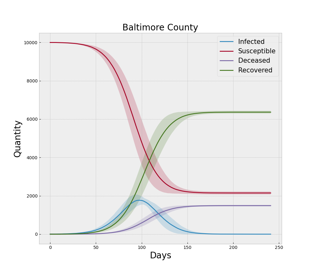
In the context of the ABM and COVID-19, the original form of the model is an extension of the canonical SEIR model where the assumptions of continuity are relaxed in favor of discrete agents and the concepts of behavioral changes induced by NPIs are incorporated. The final form of the model is a NetLogo representation of that logic. Verification begins with ensuring that logic was written correctly for the intended results. Beyond reviewing the code for errors, much of the verification process involves running the model under extreme settings to ensure the logic responds appropriately. For example, if no agents are initially set to the Exposed state, then no outbreak will ever occur and all the agents should remain in the Susceptible state for the duration of that run. Additionally, when we run multiple replications with different random number seeds we would expect the average of the time series from each disease state to become smoother with increased replications. Thus the averaged curves would behave similar to the standard SEIR models that are dominated by the decline in the Susceptible population and the increase in the Recovered and Deceased populations. Each curve from a single replication would be more rugged than one would expect from the canonical SEIR models due to the heterogeneous mixing facilitated by the contact network. When we sum the Mild, Severe, and Critical states to make a single Infected curve, this familiar set of smooth curves is indeed reproduced qualitatively by the ABM as illustrated in Figure 3. Note the dark lines in the figure represent the mean of 30 simulation replications and the shaded areas represent one standard deviation above and below that mean.
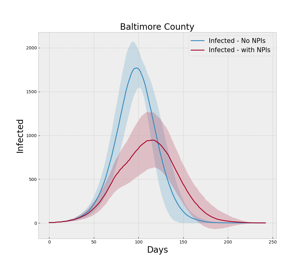
For the run generating Figure 4 we incorporate the NPIs of social distancing, testing, and tracing during the model run and note that the peak is lower than the baseline no-NPI run and the curve is rougher due to the more heterogeneous nature of social contact, which is what social distancing is designed to induce.
Proceeding in this manner we constructed a verification experiment to ensure each logical component of the model – such as testing and contact tracing – behave as intended. The heatmap shown in Figure 5 shows the interaction of different levels of testing and contact tracing for a representative dense county. As expected the two tactics interact to progressively reduce the peak number of infections and deaths.

Finally, we compared results from the simulation with the actual case counts reported in Maryland. This is a good exercise for ensuring model results are realistic, but it should be noted that precise statistical matches are not expected. There is uncertainty due to testing, the timing of NPIs, the actual adherence to NPIs, and relative scale of our 10,000 person simulations and the actual populations of a given county. Nevertheless the results shown in Figure 6 indicate that our model results reasonably represent the counties they are intended to model.

As currently implemented the model contains a number of parameters. Most of the parameters are used to define the population and its structure. There are also a number of other parameters associated with the use of NPIs and a number of parameters directly associated with the spread of the disease.
In our validation exercise the simulation demonstrated sensitivities one would expect to find in a model of this type. Disease spread was highly correlated to transmission probability and mitigation probability. Furthermore, testing made a significant difference when it was coupled with a population that complied with isolation orders. No unexpected sensitivities were uncovered, but it is important to note that SARS-Cov-2 is a novel virus and studies are producing new insights on a near daily basis. Parameterizing the model should thus remain an evolving exercise.
Experiment Design
To illustrate the utility of our modeling approach, we chose to model the 24 counties of Maryland, including the independent city Baltimore. The experiment is designed to answer the question: what is the impact of a given percent of the population being tested and a given level of participation in contact tracing if NPIs are lifted 70 days after the onset of the pandemic? This is approximately the time frame that Maryland followed when lifting NPIs in reality.
Maryland includes a mix of rural and urban counties. Baltimore and the suburbs of Washington, D.C. are the most populated areas with over 3 Million people, while Kent County has only around 19,434 inhabitants (Census 2020). Using the U.S. Census ACS data and the algorithm described earlier, we constructed the 24 contact structure graphs to represent the pre-NPIs state for initializing each simulation. The parameters used in constructing the graphs are shown in Table 2. We chose the number of agents for computational efficiency and the probabilities were taken from (Meyers et al. 2005). These graphs were ingested into the ABM as the initial contact structure.
| Parameter | Value |
|---|---|
| Total agents | \(10^4\) |
| \(P(\text{contact} | \text{household})\) | \(1.0\) |
| \(P(\text{contact} | \text{school})\) | \(3\)x\(10^{-3}\) |
| \(P(\text{contact} | \text{work})\) | \(3\)x\(10^{-4}\) |
| \(P(\text{contact} | \text{public})\) | \(3\)x\(10^{-6}\) |
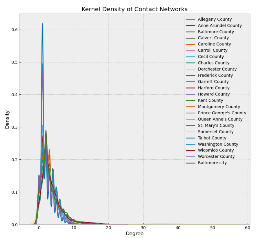
The degree distributions of each county graph are summarized by the means and standard deviations listed in Table 3 and the kernel distribution plots show in Figure 7.
| County | Mean | St. Dev | County | Mean | St. Dev | |
| Allegany County | 2.49 | 2.02 | Howard County | 2.97 | 2.21 | |
| Anne Arundel County | 2.72 | 2.09 | Kent County | 2.44 | 2.23 | |
| Baltimore County | 2.67 | 2.1 | Montgomery County | 2.8 | 2.11 | |
| Calvert County | 2.91 | 2.41 | Prince Georges County | 2.97 | 2.9 | |
| Caroline County | 2.75 | 2.53 | Queen Annes County | 2.58 | 2.05 | |
| Carroll County | 2.72 | 2.1 | St. Marys County | 2.96 | 2.28 | |
| Cecil County | 2.74 | 2.24 | Somerset County | 3.1 | 4.48 | |
| Charles County | 2.95 | 2.6 | Talbot County | 2.05 | 1.75 | |
| Dorchester County | 2.4 | 2.13 | Washington County | 2.58 | 2.15 | |
| Frederick County | 2.83 | 2.14 | Wicomico County | 3.14 | 2.82 | |
| Garrett County | 2.23 | 1.85 | Worcester County | 2.1 | 1.86 | |
| Harford County | 2.67 | 2.05 | Baltimore city | 2.71 | 2.5 |
The full experiment consisted of three sets of simulation runs. The first was a baseline run of 30 replications for each county with no NPIs or interventions. This scenario essentially represents the baseline course of the pandemic if no action were taken to slow the spread of disease. The second scenario instituted multiple NPIs 10 days after the start of each run and then partially lifted those NPIs 70 days after the start of each run. The NPIs were the closing of school and workplace venues, but not public venues. Social distancing was also enforced starting on day 10 at 95% and then reduced to 50% after 70 days. When the NPIs were lifted a strategy of testing and contact tracing was instituted. For this particular set of experiments we employed one-step contact tracing. That is, agents who came in direct contact with an infectious agent and were participating in the program were traced. But agents who came in contact with an agent who was traced were not in turn traced. In this scenario only symptomatic people were tested and contact tracing commenced for those participating cases that tested positive. Five levels of testing and five levels of agreeing to isolate after contact tracing were used for a full design of experiment consisting of 25 settings and 30 replications per county. The third scenario uses the same NPIs and timing as the second scenario, but employs a random testing strategy, which includes agents that are in the Susceptible, Exposed, Mild, or Recovered states. The same five levels of contact tracing participation were used, but the percent tested was varied across a set of higher testing levels. In our exploratory experimentation we found that higher percentages of random testing are required to achieve similar impact because the same quantity of tests uncovers fewer positive cases. This is because the symptomatic agents in the ABM only have COVID-19. Testing symptomatic cases is therefore the same as testing agents with the disease. Table 4 outlines the parameter settings for each of the three scenarios. Note that by setting social distancing to a high percentage but leaving venues open, we simulate the minimal interaction that occurs at essential businesses such as grocery stores.
| Parameter | Baseline | Symptomatic Testing | Random Testing |
| False | False | False | |
| schoolsClosedOn | never | step 20 (day 10) | step 20 (day 10) |
| schoolsClosedOff | always | step 140 (day 70) | step 140 (day 70) |
| workClosedOn | never | step 20 (day 10) | step 20 (day 10) |
| workClosedOff | always | step 140 (day 70) | step 140 (day 70) |
| socialDistanceOn | never | step 20 (day 10) | step 20 (day 10) |
| socialDistanceOff | always | never | never |
| socialDistanceProb | 0.0 | [0, 0.95, 0.5] | [0, 0.95, 0.5] |
| symptomaticTest | False | True | False |
| randomTest | False | False | True |
| percentTest | 0.0 | [0.002, 0.004, 0.006, 0.008, 0.01] | [0.002, 0.004, 0.006, 0.008, 0.01] |
| optInRate | 0.0 | [0.0, 0.25, 0.5, 0.75, 1.0] | [0.0, 0.25, 0.5, 0.75, 1.0] |
| Total Design Points | 1x24 = 24 | 5x5x24 = 600 | 5x5x24 = 600 |
| Number of Replications | 30 | 30 | 30 |
Results
In this section we review and compare the results of the different scenarios. It is important to note that these results do not represent a forecast of case counts or death rates. The purpose of this modeling approach is to provide insight into the relative impact that different NPI, testing, and tracing strategies will have when applied to areas of a particular state that have considerably different social contact structures.
Figure 8 and Table 5 show the impact of population density and social contact structure. Each box-whisker plot represents the distribution of the maximum number of infections across the 30 replications of the baseline scenario for a given county. Recall that the disease parameters are the same for each county and the populations are normalized to \(10^4\). The two variables that change from county-to-county are only the social contact structure driven by the U.S. Census data, and the population density controlled by the size of the environment the agents have to move around in. The key insight is that any strategy the state of Maryland adopts will need to treat 7 of the 24 counties differently. It is interesting to note that Harford County has roughly 75% fewer people than Montgomery County and Montgomery County is roughly 70% less dense than Baltimore City. Yet all three of these locations have an average maximum infected that is approximately four times larger than 17 of the counties in rest of the state.
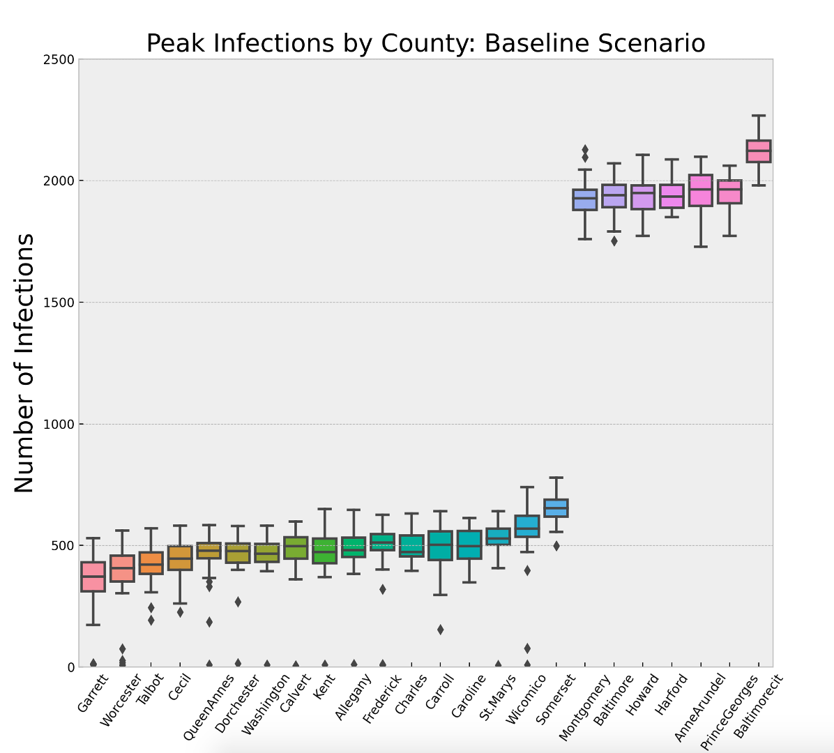
| County | Mean | St. Dev | County | Mean | St. Dev | |
| Garrett County | 340.53 | 132.95 | Carroll County | 491.13 | 103.52 | |
| Worcester County | 358.87 | 161.21 | Caroline County | 495.7 | 70.16 | |
| Talbot County | 416.03 | 81.62 | St.Marys County | 521.13 | 113.18 | |
| Cecil County | 438.67 | 80.37 | Wicomico County | 543.43 | 152.65 | |
| QueenAnnes County | 452.93 | 116.42 | Somerset County | 656.43 | 63.85 | |
| Dorchester County | 457.27 | 104.55 | Montgomery County | 1928.6 | 82.93 | |
| Washington County | 459.23 | 100.17 | Baltimore County | 1935.57 | 75.13 | |
| Calvert County | 464.5 | 138.09 | Howard County | 1938.33 | 77.1 | |
| Kent County | 472.03 | 112.4 | Harford County | 1943.83 | 60.88 | |
| Allegany County | 473.87 | 105.74 | AnneArundel County | 1949.47 | 84.8 | |
| Frederick County | 484.6 | 144.63 | PrinceGeorges County | 1953.5 | 67.57 | |
| Charles County | 490.43 | 57.57 | Baltimore City County | 2120.77 | 60.77 |
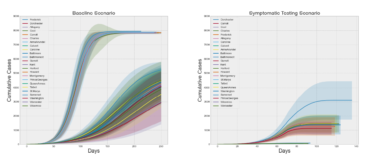
Next we analyzed the impact of a 50-day NPI strategy followed by a regime of symptomatic testing and contact tracing. From a broad perspective we can see in Figure 9 that the NPIs and testing and tracing combine to reduce the total cumulative cases considerably. Here we can see that if each county has the ability to test 1% of its population daily then the overall number of cases can be drastically reduced. Also note that, for this level of testing and contact tracing, the dynamics in Baltimore City separate from the other counties, most likely due to its extremely high density. There is still a difference from one county to the next due to the differences in density and contact structure. We selected three of the counties to look at in greater detail that are notionally representative of high, medium, and low density locations.
Baltimore City has the highest population density out of the 24 locations. Harford is seventh out of 24 in terms of density and Worcester is near the bottom. Figure 10 and Tables 6, 7, and 8 show the mean peak infections for each of the 25 design points of the symptomatic testing scenario, along with the baseline mean peak infections for each of these counties. The combined impact of the NPIs, testing, and tracing is evident, but the variation in the impact is greatly affected by the density and social contact structure of the county. It is less obvious from these plots whether different levels of testing or contact tracing have a significant effect on the mean peak infections. Indeed, using a two-sample Kolmogorov-Smirnov test with \(\alpha=0.05\) we can only reject the null hypotheses that the mean peak infections are the same when testing the baseline against the COVID-19 testing level of 0.002 and comparing that level of testing with any other level of testing for Baltimore and Harford Counties. In Worcester County all levels of testing are distinguishable from the baseline, but not from each other.

Interestingly, the story changes when we analyze deaths in these three counties within the 250 simulated days, as seen in Figure 11. The differences between certain levels of testing becomes more pronounced. Again, applying a two-sample Kolmogorov-Smirnov test to the different pair-wise combinations of testing levels we can now differentiate all pairs except the highest two levels in Baltimore and Harford County (\(\alpha=0.05\)). The levels remain indistinguishable in Worcester County. These results are important for decision-makers trying to allocate scarce resources, such as testing and contact tracing, across multiple regions of interest because the same results can be obtained in some places with fewer resources than in others.

| Baltimore City Results | |||||
| Percent Test | Opt-in Contact Trace | Mean Peak Infections | St Dev. | Mean Deaths | St Dev. |
| Baseline: 0 | Baseline: 0 | 2120.77 | 60.77 | 1492.83 | 36.49 |
| 0.002 | 0 | 1616.33 | 143.57 | 1349.74 | 53.80 |
| 0.25 | 1631.67 | 143.15 | 1366.50 | 44.74 | |
| 0.5 | 1663.03 | 152.83 | 1356.70 | 49.03 | |
| 0.75 | 1673.00 | 162.70 | 1365.50 | 49.70 | |
| 1 | 1604.03 | 301.80 | 1317.53 | 221.35 | |
| 0.004 | 0 | 1292.07 | 324.28 | 1137.20 | 142.99 |
| 0.25 | 1372.37 | 309.37 | 1178.43 | 205.63 | |
| 0.5 | 1131.10 | 428.04 | 1010.67 | 358.48 | |
| 0.75 | 1245.00 | 315.94 | 1130.17 | 216.38 | |
| 1 | 1279.97 | 375.51 | 1110.50 | 263.05 | |
| 0.006 | 0 | 1120.60 | 298.90 | 921.50 | 248.62 |
| 0.25 | 1049.41 | 433.80 | 801.97 | 349.41 | |
| 0.5 | 1069.27 | 283.91 | 874.07 | 246.01 | |
| 0.75 | 1080.83 | 358.13 | 857.40 | 272.31 | |
| 1 | 1091.87 | 315.94 | 900.67 | 239.07 | |
| 0.008 | 0 | 1038.07 | 296.12 | 707.00 | 252.90 |
| 0.25 | 998.00 | 335.28 | 678.07 | 271.98 | |
| 0.5 | 1012.43 | 298.68 | 698.57 | 241.05 | |
| 0.75 | 985.18 | 408.01 | 663.61 | 301.20 | |
| 1 | 1021.07 | 361.93 | 705.43 | 289.80 | |
| 0.01 | 0 | 911.67 | 331.05 | 538.73 | 250.77 |
| 0.25 | 1011.33 | 326.72 | 614.87 | 247.88 | |
| 0.5 | 1004.40 | 327.01 | 607.83 | 242.58 | |
| 0.75 | 931.63 | 343.79 | 556.00 | 248.95 | |
| 1 | 962.40 | 362.53 | 588.53 | 261.85 | |
| Harford County Results | |||||
| Percent Test | Opt-in Contact Trace | Mean Peak Infections | St Dev. | Mean Deaths | St Dev. |
| Baseline: 0 | Baseline: 0 | 1943.83 | 60.88 | 1481.00 | 38.47 |
| 0.002 | 0 | 1108.62 | 242.72 | 1220.90 | 227.12 |
| 0.25 | 1164.90 | 170.23 | 1260.07 | 68.15 | |
| 0.50 | 1126.00 | 207.99 | 1236.43 | 195.26 | |
| 0.75 | 1142.03 | 154.27 | 1266.37 | 62.09 | |
| 1 | 1127.70 | 165.27 | 1262.40 | 64.90 | |
| 0.004 | 0 | 628.00 | 272.13 | 610.93 | 326.14 |
| 0.25 | 702.10 | 205.18 | 721.07 | 279.82 | |
| 0.5 | 644.47 | 185.69 | 658.50 | 259.65 | |
| 0.75 | 593.17 | 209.00 | 613.13 | 296.7 | |
| 1 | 649.13 | 247.78 | 661.27 | 301.84 | |
| 0.006 | 0 | 536.83 | 183.92 | 354.80 | 175.41 |
| 0.25 | 552.13 | 175.49 | 364.33 | 181.76 | |
| 0.5 | 614.83 | 207.24 | 429.27 | 205.70 | |
| 0.75 | 598.23 | 182.03 | 416.57 | 198.25 | |
| 1 | 594.23 | 224.83 | 408.93 | 213.61 | |
| 0.008 | 0 | 586.93 | 189.63 | 333.83 | 141.39 |
| 0.25 | 564.17 | 218.69 | 324.10 | 170.46 | |
| 0.5 | 656.67 | 219.15 | 392.37 | 181.30 | |
| 0.75 | 519.63 | 176.15 | 288.53 | 121.61 | |
| 1 | 606.67 | 165.20 | 349.00 | 129.28 | |
| 0.01 | 0 | 485.67 | 174.02 | 250.80 | 112.98 |
| 0.25 | 563.13 | 190.68 | 296.20 | 131.20 | |
| 0.5 | 532.45 | 150.00 | 264.79 | 103.51 | |
| 0.75 | 592.03 | 221.39 | 314.79 | 151.94 | |
| 1 | 535.59 | 170.79 | 271.17 | 117.81 | |
| Worcester County Results | |||||
| Percent Test | Opt-in Contact Trace | Mean Peak Infections | St Dev. | Mean Deaths | St Dev. |
| Baseline: 0 | Baseline: 0 | 358.87 | 161.21 | 503.67 | 290.13 |
| 0.002 | 0 | 18.50 | 8.06 | 11.13 | 7.19 |
| 0.25 | 20.40 | 7.76 | 12.63 | 6.64 | |
| 0.5 | 18.83 | 8.73 | 11.80 | 7.98 | |
| 0.75 | 21.23 | 8.25 | 12.87 | 7.98 | |
| 1 | 18.23 | 7.78 | 10.93 | 6.63 | |
| 0.004 | 0 | 19.00 | 7.58 | 13.03 | 7.00 |
| 0.25 | 19.37 | 7.61 | 11.10 | 6.46 | |
| 0.5 | 16.20 | 4.94 | 9.23 | 4.98 | |
| 0.75 | 18.50 | 6.38 | 11.10 | 6.82 | |
| 1 | 17.47 | 9.00 | 10.27 | 7.26 | |
| 0.006 | 0 | 20.13 | 7.39 | 12.03 | 7.30 |
| 0.25 | 19.13 | 7.02 | 12.63 | 6.85 | |
| 0.5 | 18.70 | 8.38 | 11.23 | 6.10 | |
| 0.75 | 20.70 | 7.79 | 13.73 | 7.11 | |
| 1 | 19.77 | 9.13 | 13.63 | 9.61 | |
| 0.008 | 0 | 16.97 | 5.56 | 10.83 | 6.11 |
| 0.25 | 17.70 | 6.97 | 11.47 | 7.54 | |
| 0.5 | 19.43 | 9.69 | 12.47 | 7.71 | |
| 0.75 | 17.77 | 6.56 | 9.90 | 5.51 | |
| 1 | 17.13 | 7.52 | 9.67 | 4.89 | |
| 0.01 | 0 | 20.10 | 6.55 | 12.83 | 7.12 |
| 0.25 | 18.5 | 7.34 | 11.70 | 7.42 | |
| 0.5 | 19.93 | 8.45 | 12.47 | 7.04 | |
| 0.75 | 19.03 | 6.82 | 11.53 | 5.46 | |
| 1 | 19.80 | 8.46 | 12.80 | 7.94 | |
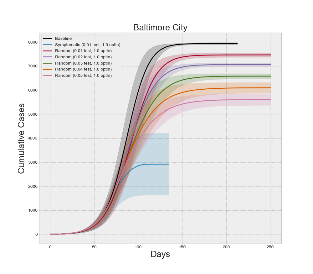
If we focus on any one county, we can analyze the interaction effects of different levels of testing and contact tracing, as well as if symptomatic or random testing produce different results. Recall that five of our design points between symptomatic testing and random testing overlap. Specifically, for all five levels of optInRate, the 1.0% testing level is included in both experiments. Holding the optInRate constant at 0.75, we can see in Figure 12 that more than 5.0% random testing is required to achieve the same results at 1.0% symptomatic testing. This result may seem misleading at first because healthcare professionals agree that more testing and random testing of asymptomatic people is highly recommended. It is important to note that all symptomatic agents in the model are indeed infected with COVID-19. So 1.0% testing of symptomatic individuals is testing a large percentage of the infectious population. Conversely, the random testing regime is forced to distribute the tests across a mix of infectious and non-infectious people. Since the non-infectious population is larger when NPIs are employed, the diluted number of true-positive tests makes the random regime appear less effective at higher levels of testing. In actuality, this reinforces the message of increased random testing. We know that many COVID-19 cases often exhibit few symptoms even though the individuals are infectious. These individuals are less likely to submit for testing because they might not even know they are sick. Increased levels of random testing provides greater opportunity of finding and isolating those cases – as illustrated by the model results – but that also means a greater level of testing is required to actually find those who are infected. It is also important to note that random testing is required to estimate the prevalence of the disease.
Discussion
In the present work, we illustrated a modeling approach for assessing alternate strategies of implementing and subsequently lifting non-pharmaceutical interventions in response to the COVID-19 pandemic. We underscored the previously-known result that social contact structure is a key factor in the size of an outbreak or pandemic and we illustrated how estimates of social contact structure combined with an agent-based model can be used to provide insight to decision-makers in the face of uncertainty. We summarized our findings in a limited design of experiments that focused on the 24 counties and county-equivalents of the state of Maryland. We showed that the different counties of Maryland fall into at least two distinct categories in terms of risk of large outbreaks and illustrated how different levels of testing can be employed to the same effect if the social contact structure is taken into account. It should be noted that the simulation is designed to enable the exploration of imposing and relaxing NPI strategies in a dynamic setting. For clarity of exposition, this initial effort focused on the imposition of NPIs to fully suppress the spread of the disease. A possible future effort could use the same model and input parameters to explore the optimal duration of a given NPI strategy or any combination of NPIs and duration.
We believe our work contributes to the ongoing struggle to contain the pandemic in the following ways. First, it is designed to be used by local governments with limited resources. This is critical for countries that delegated the decision-making to local provinces or states. Second, it is designed to use readily-available data for any region that conducts a census. Third, it is designed to be easy to use to explore the use of NPIs and inform decision-makers about how pandemic dynamics may change as a function of the timing of NPIs and the compliance of the population.
It is important to note that no model or suite of models is a panacea. Ultimately decision-makers are forced to make a choice under uncertainty to protect both the health and the economic well-being of the population. The approach outlined here is designed to provide insight into the marginal impact of one NPI and testing strategy versus another. This approach should be utilized by the decision-makers in conjunction with empirical analysis of the current state of their county or region of interest. The model parameters or logic should be constantly updated and the models re-run with new information as it comes available. That is, this modeling approach is designed for use in real-time alongside decision-makers at the time decisions are being formulated and implemented. To that end, the analysis presented here should be taken as notional rather than indicative of what might or might not happen in Maryland over the coming months.
During the writing of this report, unforeseen events extraneous to COVID-19 led to social unrest, protests, and riots in many major cities across the United States. Most of these locations were still operating under some level of restrictions to control the pandemic. Clearly, protests and riots bring people into close proximity and may ultimately prove to be super-spreading events. This sort of unpredictable event is not included in our model nor have we seen them included in the models we reviewed. This serves to underscore the difficulty and challenges of forecasting the progression of complex systems. Models and the insights they provide can help, but they are ultimately limited by assumptions. Decision-makers therefore require a combination of reliable data from their region of interest, rigorously designed models that make as few simplifying assumptions as possible, and ultimately the fortitude to make a decision in the face of uncertainty.
References
AXTELL, R. (2000). Why agents? On the varied motivations for agent computing in the social sciences. Center on Social and Economic Dynamics Brookings Institution.
BANSAL, S., Grenfell, B. T., & Meyers, L. A. (2007). When individual behaviour matters: Homogeneous and network models in epidemiology. Journal of the Royal Society Interface, 4(16), 879–891. [doi:10.1098/rsif.2007.1100]
BUREAU of Economic Analysis (2020). U. S. Bureau of Economic Analysis. Available at: https://www.bea.gov/index.php/news/glance.
BUREAU of Labor and Statistics. (2020). U. S. Bureau of Labor and Statistics. Available at: https://data.bls.gov/timeseries/LNS14000000.
BUSS, S., Papadimitriou, C. H., & Tsitsiklis, N. (1990). On the predictability of coupled automata: An allegory about Chaos. Proceedings [1990] 31st Annual Symposium on Foundations of Computer Science. [doi:10.1109/fscs.1990.89601]
CDC COVID-19 Response Team, Chow, N., Fleming-Dutra, K., Gierke, R., Hall, A., Hughes, M., Pilishvili, T., Ritchey, M., Roguski, K., Skoff, T. & Ussery, E. (2020). Preliminary estimates of the prevalence of selected underlying health conditions among patients with Coronavirus disease 2019— United States, February 12 - March 28, 2020. Morbidity and Mortality Weekly Report, 69(13), 382–386.
CENSUS, U. (2020). About the American Community Survey. Available at: https://www.census.gov/programssurveys/acs/about.html.
COWAN, G. A. (1999). 'Conference opening remarks.' In Complexity: Metaphors, Models and Reality (pp. 1–4). New York, NY: Perseus Books.
EPSTEIN, J. M. (2006). Generative Social Science: Studies in Agent-Based Computational Modeling.. Princeton, NJ: Princeton University Press. [doi:10.23943/princeton/9780691158884.003.0003]
EUBANK, S., Eckstrand, I., Lewis, B., Venkatramanan, S., Marathe, M. & Barrett, C. L. (2020). Commentary on Ferguson, et al.,“Impact of non-pharmaceutical interventions (NPIs) to reduce COVID-19 mortality and healthcare demand”. Bulletin of Mathematical Biology, 82(4), 1–7. [doi:10.1007/s11538-020-00726-x]
GALEA, S., Riddle, M., & Kaplan, G. A. (2010). Causal thinking and complex system approaches in epidemiology. International Journal of Epidemiology, 39(1), 97–106. [doi:10.1093/ije/dyp296]
GOPINATH, G. (2020). The Great Lockdown: Worst economic downturn since the Great Depression. Available at: https://blogs.imf.org/2020/04/14/the-great-lockdown-worst-economic-downturn-since-the-greatdepression.
HUANG, C., Wang, Y., Li, X., Ren, L., Zhao, J., Hu, Y., Zhang, L., Fan, G., Xu, J., Gu, X., Cheng, Z., Yu, T., Xia, J., Wei, Y., Wu, W., Xie, X., Yin, W., Li, H., Liu, M., Xiao, Y., Gao, H., Xie, J., Wang, G., Jiang, R., Gao, Z., Jin, Q., Wang, J. & Cao, B. (2020). Clinical features of patients infected with 2019 novel coronavirus in Wuhan, China. The Lancet, 395(10223), 497–506. [doi:10.1016/s0140-6736(20)30183-5]
JOHNS Hopkins University. (2020). Coronavirus Resource Center. Available at: https://coronavirus.jhu.edu.
LAUER, S. A., Grantz, K. H., Bi, Q., Jones, F. K., Zheng, Q., Meredith, H. R., Azman, A. S., Reich, N. G. & Lessler, J. (2020). The incubation period of coronavirus disease 2019 (COVID-19) from publicly reported confirmed cases: Estimation and application. Annals of Internal Medicine, 172(9), 577–582. [doi:10.7326/m20-0504]
MANZO, G. (2020). Complex social networks are missing in the dominant COVID-19 epidemic models. Sociologica, 14(1), 31–49.
MANZO, G., & Rijt, A. van de. (2020). Halting SARS-CoV-2 by targeting high-contact individuals. Journal of Artificial Societies and Social Simulation, 23(4), 10: https://www.jasss.org/23/4/10.html. [doi:10.18564/jasss.4435]
MEYERS, L. A., Pourbohloul, B., Newman, M. E., Skowronski, D. M., & Brunham, R. C. (2005). Network theory and SARS: Predicting outbreak diversity. Journal of Theoretical Biology, 232(1), 71–81. [doi:10.1016/j.jtbi.2004.07.026]
MITCHELL, M. (2009). Complexity: A Guided Tour. Oxford, NY: Oxford University Press.
NEWMAN, M. E. (2002). Spread of epidemic disease on networks. Physical Review E, 66(1), 016128.
NISHI, A., Dewey, G., Endo, A., Neman, S., Iwamoto, S. K., Ni, M. Y., Tsugawa, Y., Iosifidis, G., Smith, J. D., & Young, S. D. (2020). Network interventions for managing the COVID-19 pandemic and sustaining economy. Proceedings of the National Academy of Sciences, 117(48), 30285–30294. [doi:10.1073/pnas.2014297117]
ROTHAN, H. A., & Byrareddy, S. N. (2020). The epidemiology and pathogenesis of coronavirus disease (COVID-19) outbreak. Journal of Autoimmunity, 109, 102433. [doi:10.1016/j.jaut.2020.102433]
SANCHE, S., Lin, Y. T., Xu, C., Romero-Severson, E., Hengartner, N. W. & Ke, R. (2020). The novel coronavirus, 2019-nCoV, is highly contagious and more infectious than initially estimated. ArXiv preprint. Available at: https://arxiv.org/abs/2002.03268. [doi:10.1101/2020.02.07.20021154]
SARGENT, R. G. (2013). Verification and validation of simulation models. Journal of Simulation, 7(1), 12–24.
SQUAZZONI, F., Polhill, J. G., Edmonds, B., Ahrweiler, P., Antosz, P., Scholz, G., Chappin, É., Borit, M., Verhagen, H., Giardini, F., & Gilbert, N. (2020). Computational models that matter during a global pandemic outbreak: A call to action. Journal of Artificial Societies and Social Simulation, 23(2), 10: https://www.jasss.org/23/2/10.html. [doi:10.18564/jasss.4298]
WANG, D., Hu, B., Hu, C., Zhu, F., Liu, X., Zhang, J., Wang, B., Xiang, H., Cheng, Z., Xiong, Y., Zhao, Y., Li, Y., Wang, X. & Peng, Z. (2020a). Clinical characteristics of 138 hospitalized patients with 2019 novel coronavirus-infected pneumonia in Wuhan, China. JAMA, 323(11), 1061–1069. [doi:10.1001/jama.2020.1585]
WANG, L., Gao, Y.-H., Lou, L.-L. & Zhang, G.-J. (2020b). The clinical dynamics of 18 cases of COVID-19 outside of Wuhan, China. European Respiratory Journal, 55(4), 2000398. [doi:10.1183/13993003.00398-2020]
WILENSKY, U. (1999). NetLogo. IL: Center for connected learning and computer-based modeling, Northwestern University.
WILENSKY, U., & Rand, W. (2015). An Introduction to Agent-Based Modeling: Modeling Natural, Social, and Engineered Complex Systems with NetLogo.. Cambridge, MA: MIT Press.
WU, Z. & McGoogan, J. M. (2020). Characteristics of and important lessons from the coronavirus disease 2019 (COVID-19) outbreak in China: Summary of a report of 72314 cases from the Chinese Center for Disease Control and Prevention. JAMA, 323(13), 1239–1242. [doi:10.1001/jama.2020.2648]