The Use of Surrogate Models to Analyse Agent-Based Models

, ,
and
aBiometris, Wageningen University and Research, Netherlands; bWageningen University and Research, Netherlands; cLaboratory of Geo-Information and Remote Sensing, Wageningen University and Research, Netherlands; dBiometris, Wageningen University and, Netherlands
Journal of Artificial
Societies and Social Simulation 24 (2) 3![]()
<https://www.jasss.org/24/2/3.html>
DOI: 10.18564/jasss.4530
Received: 25-Oct-2019 Accepted: 02-Mar-2021 Published: 31-Mar-2021
Abstract
The utility of Agent Based Models (ABMs) for decision making support as well as for scientific applications can be increased considerably by the availability and use of methodologies for thorough model behaviour analysis. In view of their intrinsic construction, ABMs have to be analysed numerically. Furthermore, ABM behaviour is often complex, featuring strong non-linearities, tipping points, and adaptation. This easily leads to high computational costs, presenting a serious practical limitation. Model developers and users alike would benefit from methodologies that can explore large parts of parameter space at limited computational costs. In this paper we present a methodology that makes this possible. The essence of our approach is to develop a cost-effective surrogate model based on ABM output using machine learning to approximate ABM simulation data. The development consists of two steps, both with iterative loops of training and cross-validation. In the first part, a Support Vector Machine (SVM) is developed to split behaviour space into regions of qualitatively different behaviour. In the second part, a Support Vector Regression (SVR) is developed to cover the quantitative behaviour within these regions. Finally, sensitivity indices are calculated to rank the importance of parameters for describing the boundaries between regions, and for the quantitative dynamics within regions. The methodology is demonstrated in three case studies, a differential equation model of predator-prey interaction, a common-pool resource ABM and an ABM representing the Philippine tuna fishery. In all cases, the model and the corresponding surrogate model show a good match. Furthermore, different parameters are shown to influence the quantitative outcomes, compared to those that influence the underlying qualitative behaviour. Thus, the method helps to distinguish which parameters determine the boundaries in parameter space between regions that are separated by tipping points, or by any criterion of interest to the user.Introduction
Agent-based models (ABMs) are used for a wide range of applications (Macal 2016) and with various aims (Edmonds et al. 2019). The most common aim (Heath et al. 2009) is ‘explanation’, i.e., using the ABM to assess whether modelled interactions provide possible explanations for an observed phenomenon. When using ABMs for explanation, sensitivity analysis is needed for two reasons. First, explanations may be tested by using sensitivity analysis to vary relevant parameters. For example, Brown & Robinson (2006) tested the hypothesis that heterogeneous agent preferences in an ABM of residential development can explain observed patterns of sprawl. In this study, sensitivity analysis revealed that increasing heterogeneity does indeed increase the amount of sprawl, confirming their hypothesis. Second, sensitivity analysis is used to assess the robustness of an explanation (Grimm & Berger 2016). If the phenomenon to be explained depends on unrelated parameters, the explanation might need revision, or alternative explanations may be involved. Thus, we need to test robustness of the explanation to parameter changes. For example, in the Schelling model social segregation emerges under relatively small intolerances for neighbours of a different type (Schelling 1969). Sensitivity analysis has shown robustness of this emergence to changes in a number of assumptions and parameters, increasing the relevance of the model as explanation (Gilbert 2002; Grimm & Berger 2016). ABMs are not often used to make quantitative predictions (Heath et al. 2009), but when they are, sensitivity analysis is needed to reveal uncertainty of model predictions, and assess which parameters contribute most to this uncertainty (Ligmann-Zielinska et al. 2014). Note that this kind of assessment considers only uncertainty of predictions due to uncertain parameters, which is one out of multiple sources of uncertainty (Kwakkel et al. 2010; Walker et al. 2003).
The main strength of ABMs is that they allow for modelling a wide range of features, such as heterogeneous agents, local interactions, and various kinds of agent adaptation and learning. These features can lead to complex behavioural structures, enabling for instance, tipping points, adaptation of populations, and resilience. While this makes ABMs ideally suited for modelling complex adaptive systems, it also makes it challenging to perform sensitivity analysis. Extensive exploration of ABM parameter space is usually not practical due to the large number of parameters, high computational costs per model run, and strongly nonlinear relations between parameters and model outcomes. As a result, it is especially difficult to show robustness of model results, or uncertainties of model predictions. Thus, it is an important challenge to analyse ABMs by efficiently exploring different parameter settings and extracting relevant information from the simulation results (Crooks et al. 2008; Filatova et al. 2016; Macal 2016).
Sensitivity analysis is an essential tool to analyse ABMs. One-factor-at-a-time sensitivity analysis is a good tool for assessing effects of individual parameters. Furthermore, it can reveal the existence of tipping points in parameter space, thus helping to distinguish qualitatively different types of model behaviour. In fields like ecology, systems biology, economics, or physics, distinguishing these behaviours is considered to be an important aim, and specialised tools for bifurcation analysis are available (Kuznetsov 1998). For example, in ecology bifurcation analysis may be used to assess whether or not populations will go extinct, or show cyclic behaviour. For ABMs bifurcation analysis tools are not applicable and the main tool for model analysis is sensitivity analysis (Ten Broeke, Van Voorn, & Ligtenberg 2016). But, while one-factor-at-a-time sensitivity analysis is to some extent helpful for revealing different types of model behaviour, it ignores interaction effects (Ligmann-Zielinska et al. 2020). Variance-based global methods (Sobol 2001) can assess interaction effects over an ABM‘s entire parameter space and rank influential parameters based on their contribution to model output variance. However, these methods have two important limitations. First, the ABM outputs are aggregated without regarding the behaviour that underlies these outcomes. Thus, variance-based sensitivity analysis methods give little insight into what types of behaviour the model produces, which parameters determine the type of behaviour, or to what extent behaviour is robust (Magliocca et al. 2018; Ten Broeke et al. 2016). Thus, these methods do not really help to ’open the black box’ (Lorscheid et al. 2012) of ABMs. Second, the computational costs of gaining accurate variance-based sensitivity estimates are often prohibitive. These might be reasons why most ABM studies do not include a systematic sensitivity analysis (Thiele et al. 2014).
In this paper, we present a method for sensitivity analysis that addresses the above limitations by using surrogate models. Surrogate models can provide a way to explore ABM parameter space while keeping computational costs managable (Dosi et al. 2018; Edali & Yücel 2018; Most & Will 2011). The idea is to scan parameter space, and to fit a surrogate model to the resulting simulation data. Preliminary versions of the surrogate model are used to assess where in parameter space additional simulation data should be gathered to improve the surrogate model’s performance. Once the performance is sufficient, the surrogate model is used to generate additonal simulation data. In this paper, we will use support vector machines (SVMs) and support vector regression (SVR) as surrogate models. Both are machine learning techniques that are frequently used in Big Data applications (Bennett & Campbell 2000). Other classification or regression methods may be considered instead of SVM or SVR. Our main reasons for using SVM and SVR are that they are relatively simple, and known to be very flexible for fitting different kinds of relationship between input and output. SVM and SVR surrogate models allow for the estimation of large amounts of simulation data at much lower computational costs than the ABM. We use this data to compute sensitivity indices that would be too costly without a surrogate model. Preliminary versions of the surrogate model are also used to predict where in parameter space additional samples are needed, thus helping to further control the computational costs.
Surrogate models have been previously used as a tool for sensitivity analysis. For example, Edali & Yücel (2018) fitted a SVR model to a simple traffic ABM. Van Strien et al. (2019) have fitted an SVM to identify stable and unstable equilibria in an ABM of land-use change in a Swiss mountain region. They used the SVM to generate bifurcation diagrams that give insight into the resilience of the case-study. These results confirm that SVR and SVM can be suitable surrogate models for ABM. Other types of machine learning surrogate models have also been applied to ABM. For example, Lamperti et al. (2018) have demonstrated the use of decision trees for calibration of ABMs, and Barde & Van Der Hoog (2017) have proposed the use of Kriging metamodels for empirical validation of ABMs. Several studies have used a Bayesian approach to demonstrate the use of Gaussian processes for calibration (Ciampaglia 2013; O’Hagan 2006) and sensitivity analysis (O’Hagan 2006; Parry et al. 2013) of ABMs. The novelty of our approach lies in the combination of qualitative and quantitative analysis.
Our method consists of two steps. In the first step, we classify ABM simulation data (e.g., using SVM) into distinct behavioural regimes for which the ABM behaviour is different according to a pre-defined criterion. This criterion might distinguish regions separated by a tipping point, or can represent any quality of interest to the model user. For example, in this paper behavioural regimes will correspond to whether or not a population goes extinct, i.e., similar to a bifurcation diagram. We then compute sensitivity indices to show how robust this behaviour is to parameter changes. In the second step, we use a regression method (e.g., SVR) to assess quantitative differences within a regime, and estimate which parameters are influential. In this way, our method yields additional insight over methods of global sensitivity analysis, which aggregate across parameter space as a whole without considering qualitative differences in underlying model behaviour. While such an approach does show which parameters are influential overall, it often remains unclear in what way they are influential (Ten Broeke, Van Voorn, Kooi, et al. 2016). Our approach improves upon this, by distinguishing between whether a parameter is influential in driving the model towards a certain behavioural regime (e.g., extinction), or whether it is influential on the quantitative behaviour within the regime. Furthermore, using a surrogate model that divides parameter space in regions to accurately predict ABM output also helps to decrease the computational costs of global sensitivity analysis.
We apply the method proposed in this paper to analyse three case studies. The first case study is a differential equation model of predator-prey interaction. ABMs similar to this differential equation model have been discussed in scientific literature (Colon et al. 2015). Here we have chosen the differential equation model because of its simplicity, and because it has already been thoroughly analysed (Van Voorn et al. 2007). Both ABM versions and differential equation versions of the model contain tipping points beyond which the population goes extinct. Furthermore, it has been previously shown how these tipping points affect global sensitivity analysis results (Ten Broeke, Van Voorn, Kooi, et al. 2016). The second case study is an ABM in which agents compete in a spatial environment for a common-pool resource (Ten Broeke, Van Voorn, & Ligtenberg 2016). The third case study is an ABM of a Philippine tuna fishery system (Libre et al. 2015). Like the differential equation model, both ABMs have tipping points where the system collapses due to over-exploitation. The resource-consumer model has a relatively high level of abstraction, whereas the fishery model is a more concrete case study. For all three case studies, we demonstrate how SVM can be used to locate tipping points, which separate different behavioural regimes. Next, we use SVR to further investigate model behaviour within the region of parameter space for which the system does not collapse. In the Methods Section we describe the machine learning and sensitivity analysis techniques used in this paper. The Model Description Section gives a summarised description of the ABM test cases. The Results Section describes the results of applying SVM and SVR to analyse these test cases. The Discussion Section discusses the insights gained from applying the approach, and describes the strengths and limitations of the proposed method versus current methods of ABM analysis.
Methods
Our approach consists of two main parts. In the first part we classify the ABM’s output into different behavioural modes, and determine which parameters drive the ABM towards these behavioural modes. We assume here that the behavioural modes are defined in advance based on the interests of the modellers. Thus, the modellers need to already have some knowledge of what kind of behaviour can be produced by the model. This knowledge can for instance be obtained by performing an OFAT analysis (Ten Broeke, Van Voorn, & Ligtenberg 2016). For the examples in this paper, the criterion is whether or not the system goes to extinction, but any other criterion could be used instead. ABM output is compared directly to this criterion to determine to which behavioural mode model runs belong. An alternative approach would be to use an automated technique, such as a clustering procedure (Edali & Yücel 2019). This approach would help the modeller to explore what kind of behaviour the ABM generates without any pre-defined criterion, and would make the method applicable without having knowledge of the behaviour produced by the model. In the second part, we zoom in on a specific behavioural mode and we determine which parameters strongly affect the output. In this step, we apply a surrogate model to predict continuous ABM output. The approach is summarised in Figure 1 and discussed in more detail in the following paragraphs.
Sampling ABM parameter space
To train a surrogate model, we need a training set of sampled ABM parameter settings and corresponding output. To each parameter we assign a probability density function that represents the range over which we want to explore its effects (see e.g., Ligmann-Zielinska et al. (2014)). We draw a sample from these density functions using a replicated Latin hypercube design (McKay et al. 1979) to achieve balanced coverage of parameter space.
For the case studies in this paper, we will use an initial training sample of 1000 points. If the initial training sample does not yield sufficient performance of the surrogate model, we add additional sample points to the training sample using the adaptive sampling procedure described by Xu et al. (2014). The main idea is to draw additional sample points in the vicinity of sample points in which the surrogate model shows large prediction errors. In this way, the sampling density is increased in regions where the ABM dynamics show high activity. More precisely, for each iteration of the procedure, a large (100 times the size of the training sample) pool of sample points is generated. Each of these sample points is assigned to the closest training sample point based on Euclidian distance in parameter space. We then select a number of training sample points for which the prediction errors are largest (we use a batch size of 20). For each of these training sample points, we select a single sample point from the pool that was assigned to it. This sample point is added to the training set. The process continues either until the surrogate model fits sufficiently well (an F1 score exceeding 0.9 for classification, or a coefficient of prognosis exceeding 0.9 for regression), or until a maximum number of model runs has been performed. This maximum number of runs will usually depend on the computational costs of the ABM. For our three case studies, the details are provided in Sections 4.1, 4.6 and 4.11 respectively. In addition to the training sample we also draw a test sample, using replicated Latin hypercube sampling. This test sample remains the same throughout the analysis, and allows to test the performance of the surrogate model on an independent sample. For each of the case studies we use a test sample size of 1000 model runs.

Support vector machines
We use SVM surrogate models to classify ABM output into behavioural modes. Here we summarise the main ideas. A more thorough description of SVMs can be found in Appendix A and Ng (2008). For implementation we have used the e1071 package in R (Meyer et al. 2018). While we consider classification into two behavioural modes, the method can be extended to multiple modes by training a separate SVM for each mode. We write \({\bf x}'\) for the training sample of ABM parameters, and \({\bf y}'\) for the corresponding behavioural mode. The index \(i\) refers to specific sample points \({\bf x}'_i\) and their corresponding behavioural mode \(y'_i\) . The criterion for classification is
| \[h\left({\bf x}\right) = \left \{ \begin{array}{ll} -1 & \mbox{if $ \sum _{i=1}^m a_i y'_i K({\bf x}'_i , {\bf x}) + b \geq 0$} \\ 1 & \mbox{if $ \sum _{i=1}^m a_i y'_i K({\bf x}'_i , {\bf x} ) + b < 0.$} \\ \end{array} \right.\] | \[(1)\] |
Here, we write \({\bf x}\) for a parameter setting to be classified, \(h({\bf x})\) for the corresponding SVM prediction, and \(m\) for the number of training sample points. Note that the point \(\bf{x}\) to be classified differs from the training set \({\bf x}'\). The SVM prediction is based on the similarity between both, which is measured by the kernel function \(K({\bf x}'_i , {\bf x} )\). A weight \(a _i\) is assigned to each training sample point. Training consists of optimising the values of \(a _i\) and \(b\) such that the training sample points are classified correctly. Choosing a good sample size \(m\) is crucial for training the surrogate. As discussed in Section 2.3, we will start with \(m=1000\), but will increase the sample size over a number of iterations if needed.
For \(K({\bf x}'_i,{\bf x})\), any symmetric positive semi-definite function may be used (Ng 2008). The Gaussian kernel is the most common choice because it has been shown to perform well for many applications (Hsu et al. 2003). For this paper we have compared the performance of the Gaussian kernel against several other commonly used kernel functions, and we indeed find that the Gaussian kernel yields the best performance (Appendix C). So, throughout this paper we will use the Gaussian kernel,
| \[K({\bf x}'_i , {\bf x}) = \exp\left(-\frac{1}{2\sigma ^2} \| {\bf x}'_i - {\bf x} \|^2 \right). \] | \[(2)\] |
Support vector regression
We use SVR surrogate models to predict real-valued output data for some behavioural mode. This allows us to zoom in on a region of parameter space identified using SVM, and to investigate which parameters affect model output within this region the most. The prediction is given as
| \[f({\bf x}) = \sum _{i=1}^m (a_i - a_i^{\ast})K({\bf x}'_i , {\bf x}) + b .\] | \[(3)\] |
Cross-validation and testing
Both SVM and the SVR can be tuned by choosing the values of a few ‘meta-parameters’, which yields great flexibility for fitting a wide range of functions (Appendix A). But, these values should be chosen such that overfitting or underfitting are avoided. To this end we use fivefold cross-validation. The training set is split randomly in five equal parts. Four parts are recombined and used as training set, for a given set of meta-parameter values. The remaining part serves to assess the performance of the surrogate model. This is repeated five times, so that each of the five parts once serves to assess the performance. The meta-parameter values that on average yield the best performance are selected. The main idea behind this procedure is to avoid over-fitting by using independent samples for choosing meta-parameter values and training the surrogate model.
Sensitivity measures
We use sensitivity indices for two aims. The first aim is to indicate which parameters drive the model towards a behavioural mode. The second aim is to zoom in on one behavioural mode, and indicate which parameters strongly affect model output within this mode. A priori, we cannot know whether the same parameters are influential for both aims. Potentially, some parameters might influence the location of the border between behavioural modes, whereas other influence the quantitative results within a behavioural mode. Therefore, we use different indices to measure the contribution of each parameter for both aims.
When determining which parameters drive the model towards a behavioural mode, the model outcome is a binary variable \(y({\bf x})\) that shows whether or not the behavioural mode is found for parameter settings \({\bf x}\). To indicate the sensitivity of a single parameter \(p\), we consider the conditional probability of a behavioural mode (e.g., \(y({\bf x}) = 1\)), after fixing that parameter, \(P(y({\bf x})=1 | x_p)\). If the probability strongly depends on the value of \(x_p\), this indicates that the parameter influences which behavioural mode the model will display. If, in contrast, the parameter has little effect, then the conditional probability will vary little. As sensitivity index, we use the total range over which the conditional probability varies
| \[S_{p} = \max_{x_p} \left(P(y=1|x_p)\right) - \min_{x_p}(P( y = 1|x_p)). \] | \[(4)\] |
The second type of sensitivity index assesses the quantitative effect of a parameter within a behavioural mode. A choice for this could be the standard variance-based sensitivity index as proposed by Sobol (2001; Saltelli et al. 2008). This index assigns portions of variance in the output to different parameters. If fixing a parameter causes a considerable decrease in the variance of model output, the sensitivity of the model to this parameter is apparently large. If fixing the parameter does not decrease the variance, then the parameter apparently has no effect on the model output. This index is suitable when the variance is a good measure of the variation of model output, in which case the index also can be used to quantify interaction effects. However, for some models the variance is not a good measure for output variation, for example if the output distribution is bimodal, or contains strong outliers. This has been demonstrated for two of our case study models (Ten Broeke, Van Voorn, & Ligtenberg 2016; Ten Broeke, Van Voorn, Kooi, et al. 2016). In Ten Broeke, Van Voorn, Kooi, et al. (2016) it was shown that our first case study displays different, distinct modes of behaviour, which are separated by nonlinear boundaries in parameter space and are also dependent on initial conditions. As a result, the output is far from normally distributed, limiting the usefulness of variance-based sensitivity indices.
Several alternative indices are available that do not depend on the variance of the output distribution. Borgonovo (2007) introduced moment-free sensitivity indices that take into account the entire output distribution. Essentially, these indices are based on a comparison between the output distribution, and the conditional output distribution after fixing one parameter. This comparison is made for different values of the fixed parameter. If the fixed parameter is influential, both distributions will differ strongly on average. Entropy-based indices (Krzykacz-Hausmann 2001) are conceptually similar, but use an entropy-based measure to compare both distributions. Other possible alternatives include the DELSA method (Rakovec et al. 2014), risk-based measures (Tsanakas & Millossovich 2016), and Shapley effects (Molnar 2019). We believe any of these indices can be suitable for our method, although the reliance of DELSA on local derivatives is problematic for stochastic ABMs. A comparison between indices would be a useful topic of further study. For the present paper, we choose to use entropy-based indices (Krzykacz-Hausmann 2001) for their embedding in information theory.
The entropy \(H(Y)\) of output variable \(Y\) measures its unpredictability. Uncertain parameter values lead to output that is to some extent unpredictable. This unpredictability will decrease when parameter values are fixed. This decrease will be larger for parameters to which the model is strongly sensitive. Based on this idea, the entropy-based sensitivity is defined as,
| \[e_{p} = \frac{I(x_p,Y)}{H(Y)} = 1 - \frac{H(Y|x_p)}{H(Y)}.\] | \[(5)\] |
Equation 5 does not yield any information on interactions between \(x_p\) and other parameters. Such interactions can be relevant, because the effect of \(x_p\) may depend on the values of the other parameters. To assess parameter interactions, we propose the following index,
| \[e_p^\ast = \frac{1}{H(Y)}E_{x_{p}}\left[ H(Y|x_{\sim p})\right]\] | \[(6)\] |
Computing Equation 5 and 6 over a subset of parameter space that corresponds to a behavioural mode may cause dependencies between the model parameters. As a result, the effects of different parameters can become difficult to disentangle. For example, a parameter might be indicated as influential because it has a direct effect on the model output, but it may also be influential because it limits the range of a different parameter, which in turn affects the model output. We therefore check the correlations between parameters. If parameters are strongly correlated, there may be indirect effects like in the above example. To further account for such effects, we will compare Equation 5 and 6 to a sensitivity index based on the mean gradient of the output with respect to a parameter,
| \[g_{p} = E_{x_{\sim p}}\left[\frac{Y({\bf x}|x_p = x_{p,max}) - Y({\bf x}|x_p = x_{p,min})}{x_{p,max} - x_{p,min}} \right]\] | \[(7)\] |
The computation of above indices, especially Equation 5 (Krzykacz-Hausmann 2001) and Equation 6, requires a very large number of model runs. We therefore use the SVR surrogate model to estimate the ABM output to keep the computational costs within acceptable bounds.
Model Description
We study the following three test-cases.
Bazykin-Berezovskaya model
The Bazykin-Berezovskaya model describes the interaction between a prey population with an Allee effect and a predator population. The populations are described by an ordinary differential equation model,
| \[\frac{dY_1}{dt} = Y_1(Y_1-\zeta)(\kappa - Y_1) -Y_1Y_2\] | \[(8)\] |
| \[\frac{dY_2}{dt} = \gamma (Y_1 - h)Y_2 \] | \[(9)\] |
In this paper we show how our approach based on surrogate models can be used to deal with these tipping points in a sensitivity analysis. We consider whether or not the populations survive as distinct behavioural modes. In the first part of the analysis we will investigate under what conditions extinction occurs, and which parameters are involved. In the second part, we will focus on the region of parameter space where the populations survive. As main output we consider the population density \(Y_2\) , averaged between time-steps \(t=1000\) and \(t=5000\) to decrease the effect of oscillations on the output. We use the same parameter ranges as in Ten Broeke et al. (2016) (see Appendix D). This means that to demonstrate the method we vary the parameters \(\zeta\) and \(h\) and the initial condition \(Y_2(0)\), while keeping other parameters fixed.
Resource consumer ABM
The resource consumer ABM was previously published as a test-case for sensitivity analysis methodologies for ABMs (Ten Broeke, Van Voorn, & Ligtenberg 2016). The model is relatively simple, while still possessing essential characteristics that complicate sensitivity analysis for ABMs. The model consists of a square grid of sites on which resource grows and diffuses. Agents can move between sites and harvest from sites. Through these actions, agents compete for the resource, which they need to survive, to act, and to procreate.
The original publication (Ten Broeke, Van Voorn, & Ligtenberg 2016) includes a one-factor-at-a-time sensitivity analysis, regression-based global sensitivity analysis, and model-free global sensitivity analysis. It was concluded that the global methods yielded little insight into model behaviour because tipping points where the population goes extinct are ignored by these methods (Ten Broeke et al. 2016). In the following we show that more insight is gained by considering survival and extinction as distinct behavioural modes in our procedure. In the first part of the analysis we will investigate under what conditions extinction occurs, and which parameters are involved. In the second part, we will focus on the region of parameter space where the population survives. As main output we consider the number of agents, averaged between time-steps \(t=500\) and \(t=1000\). This averaging was done to allow for the model to converge to steady state, and to average out stochastic fluctuations. The considered parameter ranges are given in Appendix D. Both the considered output and parameter ranges are the same as those used in the previous analysis (Ten Broeke, Van Voorn, & Ligtenberg 2016).
Philippine fishery ABM
The fishery ABM was published with the aim to ‘evaluate the effects of social factors and bounded rationality on macro-level outcomes of fisheries’ (Libre et al. 2015). The spatial component of the model consists of a square grid of patches, on which fish grows and diffuses. Fishing companies, which are modelled as agents, decide yearly to buy or sell vessels. Fishing vessels, also modelled as agents, decide daily whether and where to fish. The agent behaviour of the companies and vessels are based on data from interviews with Filipino fishers. Default parameter values are based on the same interview data, as well as reports from the Philippine Bureau of Fisheries and Aquatic Resources and the Western and Central Pacific Fisheries Commission.
Previously, a one-factor-at-a-time sensitivity analysis was performed in which parameters are varied individually over a wide range (Libre et al. 2015). No global sensitivity analysis was performed. For the global sensitivity analysis in the present paper, we vary all parameters over the same range as used for the one-factor-at-a-time sensitivity analysis (Table 3). We use uniform distributions, except for some parameters of which the sum must equal one. For those parameters, we used a Dirichlet distribution to vary the individual parameters while keeping their sum constant. As main outputs we consider the total yearly profit of fishing companies and the total biomass of fish in the system. Like in the original publication, we simulate a time-span of 50 years per model run. To remove stochastic fluctuations, the output of each run is averaged over the second half of the simulation, after which the model has converged.
Results
Bazykin-Berezovskaya model
Performance of method
Both the test set and the training set consist of 1000 sample points, drawn using replicated Latin hypercube sampling. Since the model is deterministic, no replicates were used. Bifurcation analysis was used to determine analytically for which sample points the population goes extinct. This analytical outcome was used to train a SVM surrogate model to predict whether extinction occurs for sample points in the test set. We assess the performance of the SVM by its F1-score (Sasaki 2007) (Appendix D). A score of 1 would correspond to all test samples being classified correctly. Based on the training set of 1000 sample points, the surrogate model achieves an F1-score of 0.96. Thus, even without adaptive sampling the surrogate model performs well.
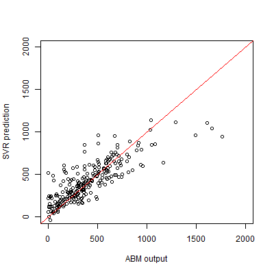
For the sample points with a non-extinct population we train an SVR surrogate model to predict the population density \(Y\). Plotting the SVR predictions against the test set output reveals a good match (Figure 3). We measure the performance of the SVR by the coefficient of prognosis (Most & Will 2011) (Appendix B) between the model output and SVR prediction. A coefficient of prognosis of 1 means that both models generate exactly the same output, while a value of 0 means that there is no correlation between the outputs. Based on the training set of 1000 sample points, we obtain a coefficient of prognosis of 0.98. Thus, the SVR accurately predicts the population density, and no sequential sampling is needed.
Classification into behavioural models
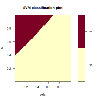
In total, 139 out of 1000 sample points in the test set maintain a positive population. The SVM predicts for which parameter settings the population goes extinct. Figure 2 shows the decision boundary as function of \(\zeta\) and \(h\) for \(y_0 = 0.1\). The population survives when \(h\) is sufficiently large, and \(\zeta\) is sufficiently small. Based on the values of the sensitivity indices \(S_p\) (Table 1) \(\zeta\) is the most important parameter for the survival of the population. But \(h\) and to a lesser extent \(Y_2(0)\) also influence survival.
Analysis of behavioural mode with surviving population
The SVR surrogate model predicts the population size for parameter settings where the population survives. The results show that when considering only the region of parameter space with a positive population, \(h\) is clearly the most influential parameter. This is true for both the first-order indices and the total-order indices. In contrast, when considering the entire parameter space, \(h\) and \(\zeta\) are approximately equally influential. This reveals that the influence of \(\zeta\) on the population size is largely explained by its influence on the tipping point where the population goes extinct. The variance-based index \(S_p\) shows \(\zeta\) to be more influential than \(h\), seemingly contradicting the values of \(e_p\) and \(e_{p,full}\). It has been previously shown that variance-based indices overestimate the contribution of \(\zeta\) compared to other indices. For a detailed discussion, we refer to Ten Broeke et al. (2016). In short, increasing \(\zeta\) leads to increased output in all parts of parameter space. Increasing \(h\) increases the output in some parts, but decreases it in other parts. Variance-based indices tend to be larger for parameters that have a consistent effect throughout parameter space. Thus, which parameter is the most influential depends on the used definition of influential.
Note that the values of \(g_p\) , which separate the effects of parameter dependencies, which are reported in Appendix E, confirm that \(h\) is the most influential parameter. The initial condition \(Y_2(0)\) can drive the population to extinction, but has no effect on the size of surviving populations, as indicated by the values of \(g_p\). This is consistent with the existence of a global bifurcation in this model (Van Voorn et al. 2007), that works as a separator of two domains of attraction. Depending on the initial condition, the population will hence persist or go extinct.

| Parameter | \(S_{p}\) | \(e_{p}\) | \(e_{p,full}\) | \(e_{p}^\ast\) | \(e_{p,full}^\ast\) | \(g_{p}\) | |||
|---|---|---|---|---|---|---|---|---|---|
| \(Y_2(0)\) | 0.21 | 0.01 | 0.05 | 0.38 | 0.06 | 0.0 | |||
| \(h\) | 0.44 | 0.38 | 0.19 | 0.69 | 0.83 | 1.8 | |||
| \(\zeta\) | 0.62 | 0.15 | 0.18 | 0.68 | 0.51 | 1.0 |
Resource consumer ABM
Performance of method
The test set for the resource-consumer ABM consists of 1000 sample points. For each points, we performed 5 replicate runs to assess the effect of stochasticity. This sample was drawn using a replicated Latin hypercube design, of 10 cubes with 100 sample points each. For a number of samples the population goes extinct. Stochasticity has little effect on the occurrence of extinction, since 99.4% of replicate pairs show the same outcome. A SVM surrogate model was trained to predict where in parameter space extinction occurs. We assess the performance of the SVM by its F1-score (Sasaki 2007) (Appendix B). A score of 1 would correspond to all test samples being classified correctly. For a replicated Latin hypercube training sample of size 1500, a score of 0.87 is achieved.
Of the variance in population size, 2.9% is explained by stochasticity, and thus cannot be captured by the SVR surrogate model. We measure the performance of the SVR by the coefficient of prognosis (Most & Will 2011) (Appendix B) between the ABM output and SVR predictions, both for replicated Latin hypercube sampling and adaptive sampling. A coefficient of prognosis of 1 means that both models generate exactly the same output, while a value of 0 means that there is no correlation between the outputs. To compare adaptive sampling to random sampling, we start with a training set of 100 sample points, and expand this set using either sampling method. The results show that adaptive sampling leads to a faster increase in the coefficient of prognosis (Figure 4). Note that for both methods the number of samples used for training is smaller than the number of drawn samples, because some of the drawn sample points result in extinction and therefore are not used for training the SVR. For the adaptive sampling, however, fewer points need to be discarded, since the use of the surrogate model helps to avoid sample points outside the region of interest. If only samples with a non-extinct population were included, the difference between both sampling methods would be smaller. For a training sample size of 1000 runs, we obtain a coefficient of prognosis of 0.83. The SVR predictions for the test set are plotted against the true values in Figure 5. While there are some deviations, especially at the extremes, the predictions generally match the ABM output well.

Classification into behavioural modes
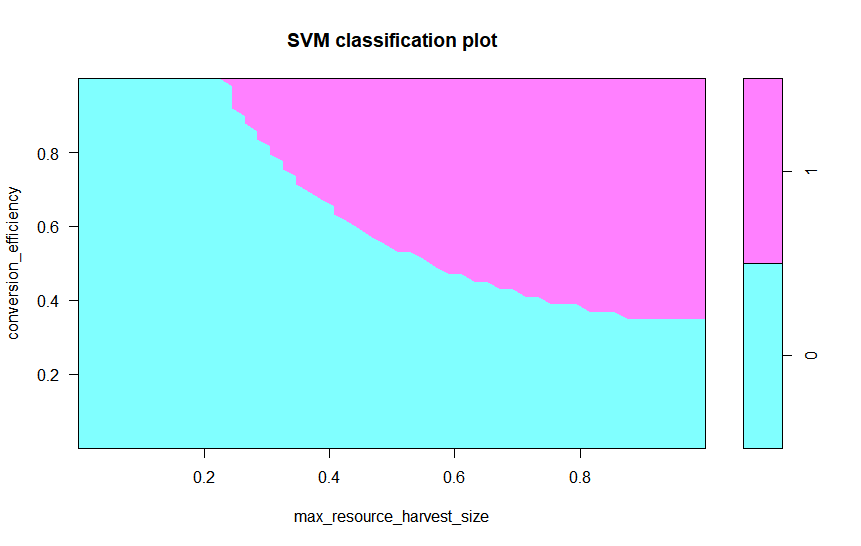
Out of 1000 sample points in the test set, 243 maintain a positive population. The SVM defines a decision boundary in parameter space beyond which the population is predicted to go extinct. This decision boundary may be visualised for any pair of ABM parameters, while keeping all other parameters fixed (similar to a bifurcation diagram) (Fig 6). Visualisation of the decision boundary is not possible when varying all parameters simultaneously, but a parallel coordinates plot (Inselberg et al. 1987) could be used to visualise which parameter combinations lead to different behavioural modes. Instead, we report the sensitivity indices \(S_{p}\) (Table 2). The indices show that the conversion efficiency, maximum resource harvest size and energy cost of harvesting strongly affect the occurrence of extinction. All of these represent bio-physical parameters involved directly in the process of harvesting resource.
Analysis of behavioural mode with surviving population
The entropy-based sensitivity indices have been estimated based on additional sample points for which the output was obtained using the surrogate model. These indices show which parameters strongly affect the size of the population if it survives. Considering only samples with surviving populations introduces correlations between the input parameters, since certain parameter combinations are more likely to lead to extinction. As discussed in the methods section, these correlations can make it difficult to disentangle the effects of different parameters in the entropy-based indices. For our model, the energy cost of harvesting is positively correlated with both the conversion efficiency, and the maximum resource harvest size. Other parameter pairs are not as strongly correlated. These pairs all have correlation coefficients with an absolute value below 0.2 (Appendix E). For the conversion efficiency, the correlation seems to lead to a low value of \(e_p\). The value of \(g_p\) shows that the parameter is influential not only on the classification, but also on the population size. The sensitivity indices show that the resource growth rate clearly has the strongest effect on population size. Thus, while this parameter has a relatively small effect on the survival of the population, it has a major effect on the size of the population, if it survives. The maximum harvest size influences both the survival of the population and the population size. Increasing this parameter increases chances of survival of the population, but decreases population size. I.e., if agents can harvest more during a time-step, this generally leads to a smaller population, but it decreases the chances of extinction.
Comparison between the indices \(S_p\), \(e_p\) and \(e_{p,full}\) reveals that generally the values of \(e_p\) and \(e_{p,full}\) show a similar pattern. The same is true for the total-order indices \(e_{p}^\ast\) and \(e_{p,full}^\ast\). Thus, for the number of agents as output the results of the analysis are similar when applying the method over the full parameter space, versus only the region that supports a population. The main contribution of our approach is that it also distinguishes which parameters determine whether the population will go extinct. For example, the agent mortality coefficient is strongly influential on whether the population goes extinct, but not on the population size. In contrast, the resource growth rate is the most influential parameter on the population size, but has little effect on the occurrence of extinction.
| Description | Dimensions | \(S_{p}\) | \(e_{p}\) | \(e_{p,full}\) | \(e_{p}^\ast\) | \(e_{p,full}^\ast\) | \(g_{p}\) | ||
|---|---|---|---|---|---|---|---|---|---|
| Initial number of agents | - | 0.05 | 0.05 | ||||||
| Initial resource per patch | mass | 0.05 | 0.04 | ||||||
| Conversion efficiency | energy mass\(^{-1}\) | 0.42 | 0.05 | 0.47 | 0.45 | 0.24 | |||
| Resource growth rate | time\(^{-1}\) | 0.26 | 0.13 | 0.84 | 0.82 | 0.48 | |||
| Resource diffusion | length\(^2\) time\(^{-1}\) | 0.27 | 0.26 | 0.09 | |||||
| Max. resource harvest size | mass | 0.42 | 0.02 | 0.20 | 0.20 | 0.10 | |||
| Energy for procreation | energy | 0.23 | 0.16 | 0.19 | 0.06 | ||||
| Observation uncertainty | mass | 0.10 | 0.10 | 0.03 | |||||
| Energy cost of harvesting | energy | 0.47 | 0.03 | 0.07 | 0.51 | 0.49 | 0.33 | ||
| Agent birth coefficient | energy\(^{-1}\) | 0.05 | 0.04 | ||||||
| Energy cost of maintenance | energy | 0.02 | 0.44 | 0.42 | 0.16 | ||||
| Agent mortality coefficient | energy\(^{-1}\) | 0.33 | 0.17 | 0.19 | 0.07 | ||||
| Energy cost of moving | energy | 0.14 | 0.13 | 0.04 | |||||
| Max. resource per patch | mass | 0.31 | 0.04 | 0.04 | 0.57 | 0.55 | 0.25 |
Fishery ABM
Performance of the method
The SVM surrogate model predicts accurately under which parameter settings the fishery disappears. For the test set of 1000 sample points, which was drawn using replicated Latin hypercube sampling, 4.6% of replicate run pairs show the same outcome. For these runs, the surrogate model cannot make accurate predictions. For 2000 training samples, an F1 score of 0.95 on the test set is achieved, showing that the surrogate model performs very well.
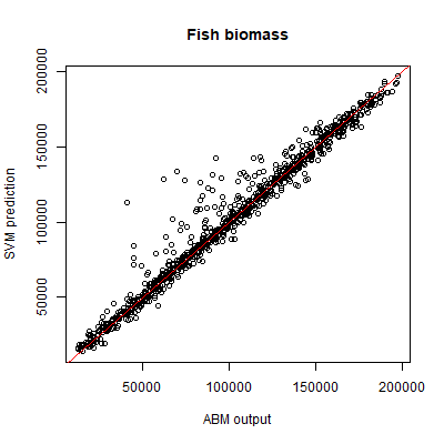
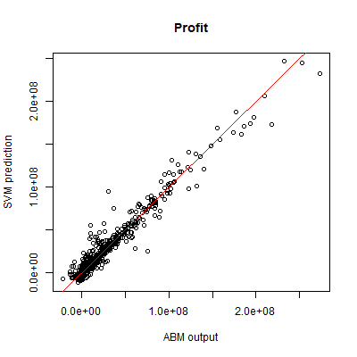
SVR was used to predict both the fish stock, and the combined yearly profit of fishing companies. We use the same 1000 sample points for the test set as for the SVM. For both outputs, stochasticity explains less than 1% of variance. Based on the same 2000 training samples that were used for the SVM, the SVR performance is very good for both outputs, as measured by a coefficient of prognosis of 0.97 for fish stock, and 0.95 for total profit. The performance is visualised by plotting the SVR predictions against the ABM output (Figures 7 and 8).
Classification into behavioural modes
We use the SVM to examine which parameters determine whether or not the fishery still exists after 50 years. In total, 886 of 1000 sample points in the test set maintain a positive number of fishing vessels. The estimated sensitivity indices (Table 3) reveal that no single parameter is as influential as some of the parameters in the other case studies. We could not find a good visualisation of the classification, since no single parameter has a strong enough effect for a clear visualisation. The indices show that the weight of available sites in P(entry) (and to some extent the other weights involved in P(entry)), the number of potential entrants, and the maximum amount of fish are relatively important parameters. Except for the maximum amount of fish, all of these parameters relate to new fishing companies starting up. Thus, controlling the influx of new companies is important for sustaining the fishery. This influx ensures that when companies go bankrupt, new companies are available to replace them.
Stock and profit
For the model runs where the fishery still exists after 50 years there are no strong correlations between parameters in the training or test set, which enables us to easily identify the effects of each individual parameter. For fish stock, the maximum amount of fish is clearly the most influential parameter. The value \(e_{p} = 0.48\) indicates that a substantial part of the uncertainty in model predictions is solely attributed to this parameter. Furthermore, the value of \(e_{p}^\ast = 0.80\) indicates that the parameter is also involved in interaction effects. A number of other model parameters are also involved in interactions. Both economic parameters, such as base skipjack price and fuel cost per liter, and ecological parameters, such as fish growth rate, are relevant. For a number of parameters, \(e_{p}^\ast =0\). This indicates that those parameters do not contribute to output uncertainty, even when considering interaction effects.
Note that parameters that strongly affect the classification (measured by the indices \(S_p\)), may not be influential on predictions of stock or profit, or vice versa. For example, while parameters related to entry of new fishing companies are among the most important parameters for existence of the fishery after 50 years, these parameters have little effect on stock or profit if the fishery persists. In contrast, skipjack price strongly affects profit of the fishery, if it continues to exist, but has little effect on whether or not it does continue to exist. The only parameter that is influential on all the considered outputs is the maximum amount of fish in the system. Differences between \(e_p\) and \(e_{p,full}\) are minor. Thus, generally the same parameters are influential for both the full parameter space, and the region where extinction does not occur. But, our method yields additional information over standard global sensitivity analysis, since it also shows which parameters affect the continued existence of the fishery, as measured by the indices \(S_p\).
| Class. | Stock | Profit | ||||||||||
|---|---|---|---|---|---|---|---|---|---|---|---|---|
| Parameter | \(S_p\) | \(e_{p}\) | \(e_{p,full}\) | \(e_{p}^\ast\) | \(e_{p,full}^\ast\) | \(g_{p}\) | \(e_{p}\) | \(e_{p,full}\) | \(e_{p}^\ast\) | \(e_{p,full}^\ast\) | \(g_{p}\) | |
| Initial no. of companies | .05 | .05 | .08 | .12 | ||||||||
| Number of potential entrants | .15 | .07 | .10 | |||||||||
| Target ratio of catch to capacity | .09 | .30 | .30 | .11 | .37 | .45 | .11 | |||||
| Average catchability | .08 | .25 | .26 | .08 | .43 | .47 | .08 | |||||
| Resistance to sell vessel | .06 | .06 | ||||||||||
| Minimum entrepreneurship | .05 | .05 | ||||||||||
| Congestion threshold | .18 | .18 | .06 | .26 | .32 | .06 | ||||||
| Weight of catch in P(buy) | .07 | .05 | .09 | |||||||||
| Weight of capital to cost in P(buy) | .07 | .07 | ||||||||||
| Weight of buying ratio in P(buy) | .05 | .11 | .06 | |||||||||
| Weight of available sites in P(buy) | .10 | .06 | ||||||||||
| Weight of entrepreneurship in P(buy) | .08 | .12 | ||||||||||
| Weight of catch in P(sell) | ||||||||||||
| Weight of earning vessels in P(sell) | .05 | |||||||||||
| Weight of buying ratio in P(entry) | .12 | .07 | ||||||||||
| Weight of catch info in P(entry) | .06 | |||||||||||
| Weight of available sites in P(entry) | .19 | .05 | .07 | |||||||||
| Starting capital | .05 | .06 | ||||||||||
| Investment costs of a vessel | .06 | .06 | ||||||||||
| Annual fixed cost per vessel | .05 | .07 | ||||||||||
| Fuel cost per liter | .09 | .09 | .37 | .43 | ||||||||
| Base skipjack price | .14 | .18 | .08 | .08 | .58 | .61 | ||||||
| Price to catch coefficient | .05 | .05 | ||||||||||
| Maximum amount of fish | .15 | .48 | .47 | .80 | .94 | .69 | .14 | .16 | .67 | .70 | .69 | |
| Initial amount of fish | .05 | .05 | ||||||||||
| Growth rate of fish | .28 | .28 | .10 | .27 | .33 | .10 | ||||||
| Diffusivity of fish | .05 | .05 |
Conclusions and Discussion
In this paper, we introduced a sensitivity analysis approach that uses surrogate models to distinguish between different behavioural modes. We demonstrated the approach using three case studies. For all three case studies, the SVM and SVR surrogate models yield good fits with the test data. Furthermore, our method yields insight into the behaviour of the models. For the Bazykin-Berezovskaya model, the method shows that different parameters affect the survival of the population and the population density. Furthermore, this case also shows that performing sensitivity analysis over the region of parameter space with a surviving population can yield different outcomes from performing a standard global sensitivity analysis over the entire parameter space. For the resource-consumer ABM a variance-based global sensitivity analysis was previously performed. Our procedure improves upon this analysis by distinguishing between runs with qualitatively different behaviour, which cannot be achieved by standard variance-based sensitivity analysis. Using our procedure, we can distinguish between parameters that impact the qualitative behaviour of the ABM, and parameters that influence the quantitative outcomes, such as the size of the population. Thus, our method gives additional information, because it shows that different parameters are important for the quantitative and qualitative outcomes. For example, the parameters for the conversion efficiency, mortality coefficient, and maximum harvest in the resource-consumer model strongly influence the occurrence of extinction, but are relatively less influential on the quantitative outcomes (Table 2). The same holds true in the fishery model for the four parameters related to entry of fishing companies (Table 3). This information could not have been obtained using standard variance-based sensitivity analysis, because that approach does not distinguish between different qualitative behaviours. Thus, our approach is especially valuable if one aims to assess, in addition to the quantitative model outcomes, transitions between different types of behaviour, and which parameters influence these transitions. We therefore believe that our approach presents one step towards addressing the need for methodologies to analysis for ABMs (Crooks et al. 2008; Filatova et al. 2016; Macal 2016). In our examples, the behavioural modes are separated by tipping points beyond which the system goes extinct, but any criterion of interest to the model user could be substituted. In some cases, like the second and third case study, the parameters that influence the quantitative behaviour within a behavioural mode may be the same as those that are influential in a standard variance-based sensitivity analysis. When comparing these indices, it is relevant to consider the sample size corresponding to the behavioural mode of interest relative to the total sample size. Other cases, like the first case study, display clear differences between the sensitivity indices. If clear differences exist, this indicates that the parameter sensitivities vary depending on the region of parameter space. Note that in particular the first case study has strong non-linearities, which may explain such differences in the sensitivity indices.
We have used entropy-based sensitivity indices to express parameter importance. This includes the index \(e_{p}\) introduced by Krzykacz-Hausmann (2001) and the index \(e_{p}^\ast\), which is based on the index \(e_p\), but was not previously used in this form. The more commonly used variance-based indices are not applicable in case of parameter dependencies, because the normalisation breaks down. Entropy-based indices provide a good alternative. Furthermore, they have the added advantage that they do not depend only on the second moment of the distribution, but on its entire shape. In addition, we have used gradient-based indices, which can separate the direct effect of a parameter on the output, from the indirect effect of limiting the range of other parameters when a subregion of parameter space is considered. Alternative sensitivity indices or visualisation methods could still be explored to express parameter importance. Our approach in this paper is mostly aimed towards global analyses where all parameters are varied simultaneously. Compared to local methods, global methods have much higher computational costs, which makes the training of a surrogate model worthwhile. An overview of global sensitivity analysis methods is given by Iooss & Lemaı̂tre (2015). Since ABMs are often strongly non-linear indices based on regression Pearson correlation coefficients or standard regression coefficients are not suitable. The indices proposed by Borgonovo (2007) could be suitable, and have a similar interpretation to the entropy-based indices in terms of first- and total-order effects. Other alternatives include risk-based measures (Tsanakas & Millossovich 2016) or the DELSA method (Rakovec et al. 2014), scatterplots can be useful, but are often difficult to interpret if the number of model parameters is large. Parallel coordinate plots can be a valuable tool for visualing the classification outcomes, or for example the 5% largest simulation outcomes. Likewise, methods to increase ‘interpretability’ of machine learning models (Molnar 2019) could also be applied. Methods like permutation feature importance and Shapley values look especially promising, and could likely be used to generate indices similar to first- and total-order indices. To evaluate the advantages and disadvantages of these different methods in more detail, a direct comparison would be needed.
Previously we have compared several standard methods of sensitivity analysis based on application to the same resource-consumer model discussed in this paper (Ten Broeke, Van Voorn, & Ligtenberg 2016). One of the main conclusions was that one-factor-at-a-time sensitivity analysis, in which parameters are varied individually across a large range, is a good starting point for sensitivity analysis of ABMs. Compared to the method discussed here, one-factor-at-a-time sensitivity analysis is computationally cheaper. Furthermore, the method shows causal effects of changes in individual parameters on the model output, and can reveal tipping points. The disadvantage is that interaction effects are not taken into account. The approach in this paper does assess interaction effects by doing a more extensive exploration of parameter space. Note, however, that the global effect of a parameter can differ strongly from its local effect around a specific point in parameter space. For example, the sensitivity indices of the fishery model show that diffusivity of fish has only a minor effect on the continued existence of the fishery. This means that in some parts of parameter space, changes in this parameter will cross a tipping point leading to disappearance of the fishery, as was noted in the original publication (Libre et al. 2015). Thus, the method presented here is not a substitute for local one-at-a-time sensitivity-analysis. Both methods give different kinds of information, and can be used to complement each other.
The present methodology requires some prior information about the model behaviour to make a classification and start up the analysis. Performing an OFAT analysis is one way to obtain information about e.g. tipping points that function as boundaries between different behavioural modes (Ten Broeke, Van Voorn, & Ligtenberg 2016). An alternative approach is to use a clustering procedure, as was done by Edali & Yücel (2018). This would make the method applicable without previous knowledge about model behaviour. It depends on the aims of the researcher which of these approaches is the most suitable. The approach in this paper is suitable if one is interested in specific behavioural modes, while a clustering procedure would be suitable if one wants to explore what behavioural modes the model can produce.
In the present paper temporal dynamics of the method are not yet covered. Computing sensitivity indices as function of time, e.g., by using a sliding window with a mean value across a small time interval, can give insight into the dynamics of ABM (Ligmann-Zielinska & Sun 2010) and this is a possible extension of the method. Machine learning techniques in particular may be helpful for gaining insight into these dynamics because they can allow us to look in more detail at simulated sample paths (Nelson 2016). While the present paper does not yet address this, by separating parameter space into regions it does present one step towards using more detailed analysis methods to gain additional insight into ABM behaviour. Furthermore, using surrogate models ensures that this additional insight over standard methods is gained at relatively low computational costs.
Model Documentation
R code for the analysis of both example models presented in our study is available as an electronic supplement (https://github.com/GuustenBroeke/ABM-surrogates). All of the simulation data used during the analysis and the NetLogo files of the ABMs is also available here. Both ABMs are also available on OpenABM (https://www.comses.net/codebases/5374/releases/1.1.0/ for the resource-consumer model, and https://www.comses.net/codebases/a5823aa6-e45c-4d2e-b930-0bf9546cd514/releases/1.0.0/ for the fishery model).Appendix
A: Support Vector Machines and Support Vector Regression
Classification
Support vector machines (SVMs) are a machine learning tool used to classify output data. While the method can be extended to deal with a larger number of categories, here we describe it for two categories, marked as -1 and 1. The classification is based on the following decision criterion,
| \[h({\bf x}) = \left \{ \begin{array}{ll} -1 & \mbox{if $ {\bf w}^T {\bf x} + b \geq 0$} \\ 1 & \mbox{if $ {\bf w}^T {\bf x} + b < 0.$} \\ \end{array} \right.\] | \[(10)\] |
Here, \(h({\bf x})\) is the SVM classification, and the vector \(\bf x\) contains any number of features to be used for classification. The vector \({\bf w}\) assigns a weight to each feature, and \(b\) is a constant.
To determine optimal values for \({\bf w}\), we need a set of training samples for which both the features and classification are known. The weights are set such that the SVM correctly predicts the classification of as many training samples as possible. This is achieved by solving the following optimisation
| \[ \begin{gathered} \min_{{\bf w}, b, {\bf \xi}} \left( \frac{1}{2}\| {\bf w} \|^2 + C \sum_{i=1}^n \xi_i \right) \\ \mbox{subject to} \left \{ \begin{array}{ll} {\bf y}_i \left({\bf w}^T{\bf x}_i + b \right) \geq 1 - \xi_i, \\ \xi_i \geq 0,\qquad\qquad\quad \ \ \qquad \qquad i=1, 2, ..., n. \end{array} \right. \end{gathered}\] | \[(11)\] |
Here \({\bf x}_i\) denotes the features of sample \(i\), and \({\bf y}_i\) the corresponding classification. It can be shown that the minimisation of the weights \(w\) ensures that the margin between the decision boundary (Equation 1) and the training samples is maximised. The constraints ensure correct classification according to Equation 1. Since correct classificaton of all samples may be impossible, slack variables \(\xi _i\) are introduced. If \(\xi _i > 0\), sample \(i\) can be misclassified while still meeting the minimisation constraints. However, this misclassification is penalised in the minimisation term. The regularisation parameter \(C\) weighs the penalty for slack variables against the minimisation of \(w\). Large values of \(C\) strongly penalise misclassification, and may lead to overfitting. Small values of \(C\) avoid overfitting, but may lead to a decreased classification accuracy.
For many applications, the linear decision criterion of Equation 1 is not suitable. An advantage of SVMs is that the linear criterion can be replaced by a number of alternative criteria. This replacement is based on the dual form of the mathematical model specified by Equation 9 and 10. This dual form is written as (Ng 2008),
| \[\begin{gathered} \max_{\bf a} \left( \sum _{i=1}^n a_i -\frac{1}{2} \sum_{i,j=1}^n y_iy_j a_i a_j \langle {\bf x}'_i,{\bf x}'_j \rangle \right) \\ \mbox{subject to} \quad \left \{ \begin{array}{ll} 0 \leq a_i \leq C \\ \sum_{i=1}^n a_i y_i = 0, \quad i=1, 2, ..., n. \end{array} \right. \end{gathered}\] | \[(12)\] |
where \(a _i\) are Lagrange multipliers. Solving the dual problem yields the same solution as solving the primal problem (Equation 10). Using the dual form, it can be shown that the decision criterion can be written as
| \[{\bf w}^T {\bf x} + b = \sum _{i=1}^m a_i y_i \langle {\bf x}'_i , {\bf x} \rangle + b. \] | \[(13)\] |
Both Equation 11 and Equation 12 depend on the inner product \(\langle {\bf x}'_i , {\bf x} \rangle\), rather than on \({\bf x}\) itself. Therefore, this inner product can be replaced by a Kernel function \(K({\bf x}'_i , {\bf x}) = \phi({\bf x}'_i)^T\phi({\bf x})\), where \(\phi ({\bf x})\) represents a feature mapping of \({\bf x}\). A necessary and sufficient condition for this replacement is that \(K({\bf x}'_i, {\bf x})\) is symmetric positive semi-definite. Furthermore, the Kernel function should measure the similarity between \({\bf x}\) and \({\bf x}'_i\). In this paper we will use a Gaussian Kernel function
| \[K({\bf x}'_i , {\bf x}) = \exp\left(-\frac{1}{2\sigma ^2} \|{\bf x}'_i - {\bf x} \|^2 \right).\] | \[(14)\] |
The value of \(K({\bf x}'_i , {\bf x})\) ranges between \(0\) and \(1\). If \(K({\bf x}'_i , {\bf x}) = 1\), both samples are identical, and \(K({\bf x}'_i , {\bf x})\) asymptotically decreases to zero as the distance between the samples increases.
Regression
While SVM is used to classify output data, support vector regression (SVR) is used to predict real-valued output data, rather than to classify data. This prediction is given as
| \[f({\bf x}) = \sum _{i=1}^n w _i K({\bf x}'_i , {\bf x}) + b,\] | \[(15)\] |
where we have used a Kernel in the same way as for SVM. To each sample \({\bf x}'_i\), a weight \(w_i\) is assigned. These weights are optimised when Equation 14 is fitted to the training data by solving the following optimisation problem
| \[ \begin{gathered} \mbox{minimise} \quad \frac{1}{2} \| {\bf w} \|^2 + C \sum_{i=1}^n (\xi _i + \xi _i^*)\\ \mbox{subject to} \quad \left \{ \begin{array}{ll} & y_i - \sum_{j=1}^n w_j K({\bf x}'_j , {\bf x}) - b \leq \epsilon + \xi _i \\ & \sum_{j=1}^n w_j K({\bf x}'_j , {\bf x}) + b - y_i \leq \epsilon + \xi _i^\ast\\ & \xi_i , \xi_i^* \geq 0. \end{array} \right. \end{gathered}\] | \[(16)\] |
The constraints ensure that if the difference between the prediction and the actual output \(y_i\) of the training data is smaller than \(\epsilon\), the sample does not contribute any cost to the objective function. If the difference is larger than \(\epsilon\), then \(\xi_i\) or \(\xi _i^\ast\) will be positive and will contribute to the objective function. Similar to SVM, we can write the dual form of the mathematical model specified by Equation 15 and 15 and choose a Kernel function.
B: Performance Measures
We assess the performance of the SVM surrogate models by its F1-score (Sasaki 2007). The score is defined as the harmonic mean of the precision and recall,
| \[\text{F1} = \frac{2 \: \text{Precision} * \text{Recall}}{\text{Precision} + \text{Recall}}.\] | \[(17)\] |
The precision is defined as
| \[\text{Precision} = \frac{tp}{tp+fp},\] | \[(18)\] |
where \(tp\) denotes the number of true positives and \(fp\) denotes the number of false positives. The recall is defined as
| \[\text{Recall} = \frac{tp}{tp+fn},\] | \[(19)\] |
where \(fn\) denotes the number of false negatives. By considering both precision and recall it is ensured that the F1-score yields a balanced performance measure, even when the numbers of positives and negatives differ strongly.
The performance of the SVR surrogate model is assessed by the coefficient of prognosis (Most & Will 2011). It is defined as
| \[\text{Coefficient of prognosis} = \left( \frac{ E[{\bf Y}({\bf x}) \cdot f({\bf x})]}{\sigma({\bf Y({\bf x})}) \sigma({f(\bf x)})} \right)^2.\] | \[(20)\] |
Here \({\bf Y}({\bf x})\) is the ABM output and \(f({\bf x})\) is the corresponding SVR prediction. Both are measured over test data that is independent from the training data used to train the SVR. A value of 1 means that the ABM output and SVR predictions are exactly equal. A value of 0 means that there is no correlation between them.
C: Choice of Kernel Function
In this Appendix we compare the performance of several Kernel functions. Included are the Gaussian, linear, polynomial (third order), and sigmoid kernels. These are the most common kernel choices, and are all the options available in the e1071 R package (Meyer et al. 2018). The performance was tested on the resource-consumer model using a Latin hypercube sample with a training set size of 3000 sample points. The results are shown in Table 4. For SVM classification, the Gaussian kernel clearly outperforms the other options. For the sigmoid kernel no score could be given, because it predicts extinction for all test samples, leading to division by zero in the F1 score. Thus, the sigmoid kernel has no predictive power at all. For SVR regression, the performance of the Gaussian, linear, and polynomial kernel are very close.
| Kernel | SVM classification | SVR regression |
|---|---|---|
| Gaussian | 0.87 | 0.70 |
| Linear | 0.39 | 0.71 |
| Polynomial | 0.39 | 0.69 |
| Sigmoid | - | 0.64 |
D: Parameter Ranges Used in Sensitivity Analysis
| Symbol | Description | Value/Range | |
|---|---|---|---|
| \(Y_1(0)\) | Initial prey population | 0.9 | |
| \(Y_2(0)\) | Initial predator population | 0.1 | 0-1 |
| \(\gamma\) | Conversion factor | 1 | |
| \(\kappa\) | Carrying capacity | 1 | |
| \(h\) | Predator mortality rate | 0 - 1 | |
| \(\zeta\) | Allee threshold (prey) density | 0 - 1 |
| Description | Dimensions | Range | |
|---|---|---|---|
| Initial number of agents | - | 1 - 200 | |
| Initial resource per patch | mass | 0 - 1 | |
| Conversion efficiency | energy mass\(^{-1}\) | 0 - 1 | |
| Resource growth rate | time\(^{-1}\) | 0 - 0.5 | |
| Resource diffusion | length\(^2\) time\(^{-1}\) | 0 - 0.1 | |
| Max. resource harvest size | mass | 0 - 1 | |
| Energy for procreation | energy | 0 - 10 | |
| Observation uncertainty | mass | 0 - 0.5 | |
| Energy cost of harvesting | energy | 0 - 0.5 | |
| Agent birth coefficient | energy\(^{-1}\) | 0 - 5 | |
| Energy cost of maintenance | energy | 0 - 0.05 | |
| Agent mortality coefficient | energy\(^{-1}\) | 0 - 5 | |
| Energy cost of moving | energy | 0 - 0.05 | |
| Max. resource per patch | mass | 0 - 5 |
| Parameter | Units | Range |
|---|---|---|
| Initial no. of companies | Companies | 0 - 49 |
| Number of potential entrants | Companies | 0 - 44 |
| Target ratio of catch to capacity | - | 0.01 - 0.99 |
| Average catchability | day\(^{-1}\) | 0.001 - 0.0015 |
| Resistance to sell vessel | - | 0 - 1 |
| Minimum entrepreneurship | - | 0 - 1 |
| Congestion threshold | - | 0 - 1 |
| Weight of catch in P(buy) | - | 0 - 1 |
| Weight of capital to cost ratio in P(buy) | - | 0 - 1 |
| Weight of buying ratio in P(buy) | - | 0 - 1 |
| Weight of available sites in P(buy) | - | 0 - 1 |
| Weight of entrepreneurship in P(buy) | - | 0 - 1 |
| Weight of catch in P(sell) | - | 0 - 1 |
| Weight of earning vessels in P(sell) | - | 0 - 1 |
| Weight of buying ratio in P(entry) | - | 0 - 1 |
| Weight of catch information in P(entry) | - | 0 - 1 |
| Weight of available sites in P(entry) | - | 0 - 1 |
| Starting capital | USD | 0 - 1.8 * 10\(^6\) |
| Investment costs of a vessel | USD | 0 - 3.0 * 10\(^6\) |
| Annual fixed cost per vessel | USD year\(^{-1}\) | 0 - 1.0 * 10\(^5\) |
| Fuel cost per liter | USD l\(^{-1}\) | 0.5 - 4.5 |
| Base skipjack price | USD | 400 - 2400 |
| Price to catch coefficient | USD ton\(^{-1}\) | -0.001 - 0.001 |
| Maximum amount of fish | ton | 1.25 * 10\(^4\) - 1.75 * 10\(^4\) |
| Initial amount of fish | ton | 0 - 1 |
| Growth rate of fish | day\(^{-1}\) | 0.0005 - 0.0085 |
| Diffusivity of fish | miles\(^{-1}\) day\(^{-1}\) | 0 - 420 |
E: Parameter correlations for behavioural mode of interest
Considering only a specific behavioural mode, rather than the whole parameter space, introduces dependencies between parameters. These dependencies can influence computed sensitivity indices, because one parameter can have an indirect effect on the output through influencing the range of other parameters. Here, we provide the correlation matrices for the model parameters for the Bazykin-Berezovskaya model, and the resource consumer ABM. The most important results are discussed in the main paper. The values here are provided so that readers can verify these results themselves. The matrices have been computed on the test samples of the corresponding case studies. For the fishery model, we do not give the full matrix, due to the large number of parameters. For this model, all of the correlations are below 0.1, except for the correlation between the target ratio of catch to capacity, and the weight of available sites in \(P(entry)\). The correlation between these two parameters equals 0.11.
| \(\zeta\) | \(h\) | \(Y_2(0)\) | |
|---|---|---|---|
| \(\zeta\) | 1 | 0.22 | -0.43 |
| \(h\) | 1 | -0.09 | |
| \(Y_2(0)\) | 1 |
| \(n_0\) | \(R_0\) | \(c\) | \(r\) | \(D\) | \(R_{max}\) | \(E_b\) | \(R_{unc}\) | \(E_h\) | \(v_b\) | \(E_m\) | \(v_d\) | \(E_{move}\) | \(z\) | \(K\) | |
|---|---|---|---|---|---|---|---|---|---|---|---|---|---|---|---|
| \(n_0\) | 1 | -0.09 | -0.00 | 0.03 | -0.04 | 0.02 | -0.01 | 0.03 | 0.06 | 0.03 | -0.01 | -0.04 | -0.12 | 0.02 | 0.01 |
| \(R_0\) | 1 | -0.01 | 0.02 | -0.01 | 0.03 | 0.12 | -0.04 | 0.02 | -0.02 | 0.08 | 0.01 | -0.06 | -0.07 | 0.03 | |
| \(c\) | 1 | 0.10 | 0.09 | -0.13 | 0.12 | -0.06 | 0.35 | -0.01 | 0.02 | -0.13 | 0.01 | 0.01 | -0.07 | ||
| \(r\) | 1 | 0.02 | -0.08 | -0.04 | -0.02 | -0.02 | -0.02 | 0.03 | -0.11 | -0.08 | -0.04 | 0.02 | |||
| \(D\) | 1 | -0.03 | 0.06 | -0.07 | -0.01 | -0.00 | -0.06 | -0.03 | 0.02 | -0.06 | -0.05 | ||||
| \(R_{max}\) | 1 | 0.02 | 0.02 | 0.33 | 0.08 | 0.01 | 0.18 | 0.02 | -0.13 | 0.07 | |||||
| \(E_b\) | 1 | -0.13 | 0.09 | -0.05 | 0.00 | -0.17 | -0.03 | 0.08 | -0.16 | ||||||
| \(R_{unc}\) | 1 | -0.13 | -0.13 | 0.06 | 0.09 | 0.01 | 0.08 | 0.07 | |||||||
| \(E_h\) | 1 | -0.05 | -0.04 | -0.05 | 0.08 | -0.07 | 0.17 | ||||||||
| \(v_b\) | 1 | 0.13 | -0.09 | -0.05 | 0.04 | -0.07 | |||||||||
| \(E_m\) | 1 | -0.05 | -0.04 | -0.03 | -0.02 | ||||||||||
| \(v_d\) | 1 | 0.04 | -0.06 | -0.06 | |||||||||||
| \(E_{move}\) | 1 | 0.02 | -0.04 | ||||||||||||
| \(z\) | 1 | 0.00 | |||||||||||||
| \(K\) | 1 |
References
BARDE, S., & Van Der Hoog, S. (2017). An empirical validation protocol for large-scale agent-based models. Bielefeld Working Papers in Economics and Management No. 04-2017 [doi:10.2139/ssrn.2992473]
BENNETT, K. P., & Campbell, C. (2000). Support vector machines: Hype or hallelujah? ACM SIGKDD Explorations Newsletter, 2(2), 1–13. [doi:10.1145/380995.380999]
BORGONOVO, E. (2007). A new uncertainty importance measure. Reliability Engineering & System Safety, 92(6), 771–784. [doi:10.1016/j.ress.2006.04.015]
BROWN, D., & Robinson, D. (2006). Effects of heterogeneity in residential preferences on an agent-based model of urban sprawl. Ecology and Society, 11(1), 46. [doi:10.5751/es-01749-110146]
CIAMPAGLIA, G. L. (2013). A framework for the calibration of social simulation models. Advances in Complex Systems, 16(04n05), 1350030. [doi:10.1142/s0219525913500306]
COLON, C., Claessen, D., & Ghil, M. (2015). Bifurcation analysis of an agent-based model for predator-prey interactions. Ecological Modelling, 317, 93–106. [doi:10.1016/j.ecolmodel.2015.09.004]
CROOKS, A., Castle, C., & Batty, M. (2008). Key challenges in agent-based modelling for geo-spatial simulation. Computers, Environment and Urban Systems, 32(6), 417–430. [doi:10.1016/j.compenvurbsys.2008.09.004]
DOSI, G., Pereira, M. C., & Virgillito, M. E. (2018). On the robustness of the fat-tailed distribution of firm growth rates: A global sensitivity analysis. Journal of Economic Interaction and Coordination, 13(1), 173–193. [doi:10.5151/engpro-1enei-058]
EDALI, M., & Yücel, G. (2018). Automated analysis of regularities between model parameters and output using support vector regression in conjunction with decision trees. Journal of Artificial Societies & Social Simulation, 21(4), 1: https://www.jasss.org/21/4/1.html. [doi:10.18564/jasss.3786]
EDALI, M., & Yücel, G. (2019). Exploring the behavior space of agent-based simulation models using random forest metamodels and sequential sampling. Simulation Modelling Practice and Theory, 92, 62–81. [doi:10.1016/j.simpat.2018.12.006]
EDMONDS, B., Le Page, C., Bithell, M., Chattoe-Brown, E., Grimm, V., Meyer, R., Montañola-Sales, C., Ormerod, P., Root, H., & Squazzoni, F. (2019). Different modelling purposes. Journal of Artificial Societies and Social Simulation, 22(3), 6: https://www.jasss.org/22/3/6.html. [doi:10.18564/jasss.3993]
FILATOVA, T., Polhill, J. G., & Ewijk, S. van. (2016). Regime shifts in coupled socio-environmental systems: Review of modelling challenges and approaches. Environmental Modelling & Software, 75, 333–347. [doi:10.1016/j.envsoft.2015.04.003]
GILBERT, N. (2002). 'Varieties of emergence.' In D. Sallach (Ed.), Social Agents: Ecology, Exchange, and Evolution (pp. 41–56). University of Chicago and Argonne National Laboratory.
GRIMM, V., & Berger, U. (2016). Robustness analysis: Deconstructing computational models for ecological theory and applications. Ecological Modelling, 326, 162–167. [doi:10.1016/j.ecolmodel.2015.07.018]
HAUSSER, J., & Strimmer, K. (2009). Entropy inference and the James-Stein estimator, with application to nonlinear gene association networks. The Journal of Machine Learning Research, 10(7).
HEATH, B., Hill, R., & Ciarallo, F. (2009). A survey of agent-based modeling practices (January 1998 to July 2008). Journal of Artificial Societies and Social Simulation, 12(4), 9: https://www.jasss.org/12/4/9.html.
HSU, C.-W., Chang, C.-C., Lin, C.-J., & others. (2003). A practical guide to support vector classification. Available at: https://www.csie.ntu.edu.tw/~cjlin/papers/guide/guide.pdf.
INSELBERG, A., Reif, M., & Chomut, T. (1987). Convexity algorithms in parallel coordinates. Journal of the ACM, 34(4), 765–801. [doi:10.1145/31846.32221]
IOOSS, B., & Lemaı̂tre, P. (2015). 'A review on global sensitivity analysis methods.' In G. Dellino & C. Meloni (Eds.), Uncertainty Management in Simulation-Optimization of Complex Systems (Vol. 59, pp. 101–122). Springer. [doi:10.1007/978-1-4899-7547-8_5]
KRZYKACZ-HAUSMANN, B. (2001). Epistemic sensitivity analysis based on the concept of entropy. In P. Prado & R. Bolado (Eds.), Proceedings of SAMO2001 (pp. 31–35). CIEMAT.
KUZNETSOV, Y. A. (1998). Elements of Applied Bifurcation Theory (Second Edition). Berlin Heidelberg: Springer-Verlag.
KWAKKEL, J. H., Walker, W. E., & Marchau, V. A. (2010). Classifying and communicating uncertainties in model-based policy analysis. International Journal of Technology, Policy and Management, 10(4), 299–315. [doi:10.1504/ijtpm.2010.036918]
LAMPERTI, F., Roventini, A., & Sani, A. (2018). Agent-based model calibration using machine learning surrogates. Journal of Economic Dynamics and Control, 90, 366–389. [doi:10.1016/j.jedc.2018.03.011]
LIBRE, S. V., Voorn, G. A. van, Broeke, G. ten, Bailey, M., Berentsen, P., & Bush, S. R. (2015). Effects of social factors on fishing effort: The case of the Philippine tuna purse seine fishery. Fisheries Research, 172, 250–260. [doi:10.1016/j.fishres.2015.07.033]
LIGMANN-ZIELINSKA, A., Kramer, D. B., Cheruvelil, K. S., & Soranno, P. A. (2014). Using uncertainty and sensitivity analyses in socioecological agent-based models to improve their analytical performance and policy relevance. PloS One, 9(10), e109779. [doi:10.1371/journal.pone.0109779]
LIGMANN-ZIELINSKA, A., Siebers, P.-O., Magliocca, N., Parker, D. C., Grimm, V., Du, J., Cenek, M., Radchuk, V., Arbab, N. N., Li, S., & others. (2020). One size does not fit all: A roadmap of purpose-driven mixed-method pathways for sensitivity analysis of agent-based models. Journal of Artificial Societies and Social Simulation, 23(1), 6: https://www.jasss.org/23/1/6.html. [doi:10.18564/jasss.4201]
LIGMANN-ZIELINSKA, A., & Sun, L. (2010). Applying time-dependent variance-based global sensitivity analysis to represent the dynamics of an agent-based model of land use change. International Journal of Geographical Information Science, 24(12), 1829–1850. [doi:10.1080/13658816.2010.490533]
LORSCHEID, I., Heine, B.-O., & Meyer, M. (2012). Opening the “black box” of simulations: Increased transparency and effective communication through the systematic design of experiments. Computational and Mathematical Organization Theory, 18(1), 22–62. [doi:10.1007/s10588-011-9097-3]
MACAL, C. M. (2016). Everything you need to know about agent-based modelling and simulation. Journal of Simulation, 10(2), 144–156. [doi:10.1057/jos.2016.7]
MAGLIOCCA, N., McConnell, V., & Walls, M. (2018). Integrating global sensitivity approaches to deconstruct spatial and temporal sensitivities of complex spatial agent-based models. Journal of Artificial Societies and Social Simulation, 21(1), 12: https://www.jasss.org/21/1/12.html. [doi:10.18564/jasss.3625]
MCKAY, M. D., Beckman, R. J., & Conover, W. J. (1979). Comparison of three methods for selecting values of input variables in the analysis of output from a computer code. Technometrics, 21(2), 239–245. [doi:10.1080/00401706.1979.10489755]
MEYER, D., Dimitriadou, E., Hornik, K., Weingessel, A., & Leisch, F. (2018). E1071: Misc functions of the department of statistics, probability theory group (formerly: E1071), TU Wien. https://CRAN.R-project.org/package=e1071.
MOLNAR, C. (2019). Interpretable Machine Learning. A Guide for Making Black Box Models Explainable. Accessible at: https://christophm.github.io/interpretable-ml-book/.
MOST, T., & Will, J. (2011). Sensitivity analysis using the metamodel of optimal prognosis. Weimar Optimization and Stochastic Days, 8, 24–40.
NELSON, B. L. (2016). ’Some tactical problems’ in digital simulation for the next 10 years. Journal of Simulation, 10(1), 2–11. [doi:10.1057/jos.2015.22]
NG, A. (2008). Support vector machines. Machine Learning.
O’HAGAN, A. (2006). Bayesian analysis of computer code outputs: A tutorial. Reliability Engineering & System Safety, 91(10–11), 1290–1300. [doi:10.1016/j.ress.2005.11.025]
PARRY, H. R., Topping, C. J., Kennedy, M. C., Boatman, N. D., & Murray, A. W. (2013). A bayesian sensitivity analysis applied to an agent-based model of bird population response to landscape change. Environmental Modelling & Software, 45, 104–115. [doi:10.1016/j.envsoft.2012.08.006]
RAKOVEC, O., Hill, M. C., Clark, M., Weerts, A., Teuling, A., & Uijlenhoet, R. (2014). Distributed evaluation of local sensitivity analysis (DELSA), with application to hydrologic models. Water Resources Research, 50(1), 409–426. [doi:10.1002/2013wr014063]
SALTELLI, A., Ratto, M., Andres, T., Campolongo, F., Cariboni, J., Gatelli, D., Saisana, M., & Tarantola, S. (2008). Global Sensitivity Analysis: The Primer. Hoboken, NJ: John Wiley & Sons. [doi:10.1002/9780470725184]
SASAKI, Y. (2007). The truth of the F-measure. Accessible at: https://www.cs.odu.edu/~mukka/cs795sum09dm/Lecturenotes/Day3/F-measure-YS-26Oct07.pdf.
SCHELLING, T. C. (1969). Models of segregation. The American Economic Review, 59(2), 488–493.
SMOLA, A. J., & Schölkopf, B. (2004). A tutorial on support vector regression. Statistics and Computing, 14(3), 199–222. [doi:10.1023/b:stco.0000035301.49549.88]
SOBOL, I. M. (2001). Global sensitivity indices for nonlinear mathematical models and their Monte Carlo estimates. Mathematics and Computers in Simulation, 55(1–3), 271–280.
TEN Broeke, G. A., Van Voorn, G. A., Kooi, B. W., & Molenaar, J. (2016). Detecting tipping points in ecological models with sensitivity analysis. Mathematical Modelling of Natural Phenomena, 11(4), 47–72. [doi:10.1051/mmnp/201611405]
TEN Broeke, G. A., Van Voorn, G. A., & Ligtenberg, A. (2016). Which sensitivity analysis method should I use for my agent-based model? Journal of Artificial Societies and Social Simulation, 19(1), 5: https://www.jasss.org/19/1/5.html. [doi:10.18564/jasss.2857]
THIELE, J. C., Kurth, W., & Grimm, V. (2014). Facilitating parameter estimation and sensitivity analysis of agent-based models: A cookbook using NetLogo and R. Journal of Artificial Societies and Social Simulation, 17(3), 11: https://www.jasss.org/17/3/11.html. [doi:10.18564/jasss.2503]
TSANAKAS, A., & Millossovich, P. (2016). Sensitivity analysis using risk measures. Risk Analysis, 36(1), 30–48. [doi:10.1111/risa.12434]
VAN Strien, M. J., Huber, S. H., Anderies, J. M., & Grêt-Regamey, A. (2019). Resilience in social-ecological systems: Identifying stable and unstable equilibria with agent-based models. Ecology and Society, 24(2), 8. [doi:10.5751/es-10899-240208]
VAN Voorn, G. A., Hemerik, L., Boer, M. P., & Kooi, B. W. (2007). Heteroclinic orbits indicate overexploitation in predator-prey systems with a strong Allee effect. Mathematical Biosciences, 209(2), 451–469. [doi:10.1016/j.mbs.2007.02.006]
WALKER, W. E., Harremoës, P., Rotmans, J., Van Der Sluijs, J. P., Van Asselt, M. B., Janssen, P., & Krayer von Krauss, M. P. (2003). Defining uncertainty: A conceptual basis for uncertainty management in model-based decision support. Integrated Assessment, 4(1), 5–17. [doi:10.1076/iaij.4.1.5.16466]
XU, S., Liu, H., Wang, X., & Jiang, X. (2014). A robust error-pursuing sequential sampling approach for global metamodeling based on Voronoi diagram and cross validation. Journal of Mechanical Design, 136(7), 071009. [doi:10.1115/1.4027161]