
Introduction
Rapid international migration of significant populations generates profound implications, within and between nations. Our motivation in this work is to develop an agent-based model (ABM) to capture the existence of such migrant and refugee flows, and to explore the effects upon urban dynamics: the dynamics of population, segregation, property prices, and regeneration.
Contemporary urban environments manifest themselves as complex, interconnected socio-technical systems. In the study of cities and their dynamics, ABMs have emerged to complement econometric models (Axtell 2016; Giffinger & Seidl 2013). ABMs have been exploited to reproduce the evolution of the urban form (Stanilov & Batty 2011), to model the urban dynamics typical of cities in the developed world, such as segregation (from Schelling 1971 onwards) and gentrification (Picascia et al. 2015), and to model dynamics typical of the megacities of the developing world, such as the emergence and evolution of informal settlements (Feitosa et al. 2011; Patel et al. 2012).
Previous works constructed a micro-level ABM, derived from the rent-gap theory (RGT)—an economic hypothesis on the dynamics of investment in housing—in an effort to model the economic mechanics of property investment along with their effects on the cultural and social diversity of urban areas. Picascia et al. (2015), whose approach we follow, examined the price dynamics triggered by different levels of capital flowing in a city and the patterns of spatial inequality that may emerge. He developed a model of housing regeneration, and applied it to a major European city (Picascia 2015). Our preliminary work Picascia & Yorke-Smith (2017) went on to make a first attempt to extend the ABM to include refugee migration, but only in the form of an abstract, stylized model.
In this article we go beyond previous models, grounding our work in the city of Beirut, Lebanon. This is a densely-populated capital of a middle-income West Asian country which, according to official estimates (Government of Lebanon & United Nations 2017; United Nations High Commissioner for Refugees 2017), has experienced a refugee influx of approaching 50% of its population in the years 2011–2015. This influx caused extreme pressure on housing, the economy and social fabric (Government of Lebanon & United Nations 2017; UN HABITAT 2014; Ward & Lewis 2020). We build the first (to our knowledge) validated ABM of metropolitan Beirut using data for population, housing prices, and property conditions. Our contribution includes devising principled indices for these factors and incorporating UNHCR-supplied data for refugees. Our model, implemented in NetLogo (Wilensky 1999), is adept to investigate the possible societal consequences and economic indicators of migration, being specifically designed to explore the interrelation of urban economic and cultural dynamics. Results of the simulation exhibit how sizeable migration of low income populations into a city impacts prices, slum locations, population density, and segregation.
The article is structured as follows. We first provide the background of our work, including the rent-gap theory, and discuss related works. We then describe our model. The following sections report the validation of the model, and scenario-driven results from it. We conclude the article with a discussion of future directions.
Background and Related Work
Agent-based modelling and simulation is regarded as an ideal tool for understanding complex socio-technical systems such as cities (North & Macal 2007). As surveyed by Huang et al. (2014), the preferred approach in most residential mobility models is to identify individual or household-level agents as the main actors and describe emerging patterns as purely bottom-up outcomes of the interaction of such agents. This approach poses a risk, in our view, of underestimating the broader economic processes that impact the urban form and constrain individual behaviour. By contrast, an area of human geography enjoying revival (Harvey 2012; Smith 1996) views the socio-spatial phenomena that shape contemporary cities—suburban sprawl, income segregation, gentrification—as consequences of the varying influx of capital towards urban systems, rather than as strictly originating from individual-based residential choices.
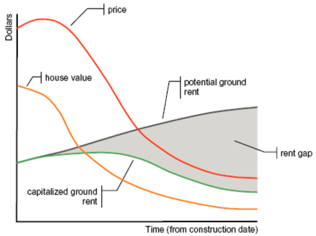
Within this theoretic lens, the rent-gap theory, from which our model draws, is a supply-side approach to housing investment. RGT is noted in economics especially for its use in studying gentrification, i.e., “the restoration and upgrading of deteriorated urban property by middle-class or affluent people, often resulting in displacement of lower-income people.” (American Heritage Dictionary). The rent gap is the difference between the actual (current) economic return from land, and the maximum potential return if the land were put to its “highest and best use” (Smith 1979). This gap is due to the decline in maintenance condition which properties undergo, together with changes in technologies which render dwellings obsolete. Restoration or rebuilding increases the economic return that a portion of land or a dwelling generates, bringing it to the maximum return possible according to the theory. The locations with the highest difference between actual and potential economic return will be the ones more likely to attract investment capital. Figure 1 depicts the rent-gap as the shaded area between the potential rent (if the land were at its highest and best use) and the actual rent (capitalized at the current use).
Although the RGT was proposed to explain a specific phenomenon—i.e., gentrification—we consider that it serves as a valid conceptualisation of general housing investment behaviour in capitalist economies, suitable for a broad exploration and not incompatible with other approaches, including standard economic theory , as pointed out by Bourassa (1993).
Indeed, the literature holds a number of ABMs inspired by the RGT in which the problem of identifying the “highest and best use” has been addressed by employing the notion of neighbourhood effect. We refer to Picascia et al. (2015) for a survey. Prior to that work, Diappi and Bolchi’s model ((2008, 2006)) was the most complete implementation of the mechanics of the RGT, although it lacks any consideration of the demand side of the housing market.
Besides models inspired by the RGT, the literature has a rich vein of ABMs that study aspects of residential mobility, either at the city level or at the national level. Among these, Ge (2013) develops an agent-based spatial model of the US housing market, obtaining “sensible aggregated outcomes that capture important characteristics in the housing market.” Zhang & Li (2014) study the housing market in Beijing, China, using an ABM built on a model of buyer and seller search behaviours; we refer to their work for a wider survey of ABMs related to housing markets. Özbaş et al. (2014) construct a systems dynamics model of housing market with the aim of understanding structural cycles in the market.
Our work applies the RGT to the city of Beirut, Lebanon. Among other disciplines, the sociology, urban design, and political economy literatures have considered the case of Beirut. The property market is neo-liberal; affordable housing is limited; public institutions are weak; regulations are rarely enforced (Ahwash 2018; Fawaz & Sabah 2015; Harb et al. 2011; Krijnen & Fawaz 2010; United Nations High Commissioner for Refugees 2016).
Beirut presents a compelling case study for at least two reasons. First, the economic and political context renders the property market ripe for the rent-gap, through both legal means and informal, illegal practices (Krijnen 2018). Second, Lebanon hosted a per-capita exceptional number of refugees during the 2010s, as we discuss later in this article, due to war in neighbouring Syria. The implications of this shock to the housing market warrant dedicated study.
We are not the first to recognize the relevance of ABM to approach the complexities and non-linearities of the socio-economic situation of Lebanon. Srour & Yorke-Smith (2016) apply agent-based simulation to study import–export processes at the Port of Beirut. Our preliminary work, Picascia & Yorke-Smith (2017) built an abstract ABM of urban dynamics of Beirut; but as noted earlier, that model is not geographically accurate, not based on housing price data, and is not validated. We do however follow these precedents and implement our ABM in the agent-based simulation platform NetLogo (Wilensky 1999).
Agent behaviour in our model is determined by the RGT and deliberately simple rules (described next). Pertinent to ABMs with more complex agent behaviours, Singh and Padgham present a paradigm for integrating agent models (particularly, for instance, models in the Belief-Desire-Intention tradition) and simulation models (particularly, technical simulation engines or social simulation platforms) (Singh & Padgham 2014). Further, Fuentes-Fernández et al. (2010) argue that, as the agents become more complex, agent-oriented software engineering practices are relevant, and present a stylizied case study of urban dynamics.
Although our focus is not on the behaviour of refugees, primarily, other works have successfully applied ABM to study migration of different forms.
First, a body of work studies refugee movement dynamics and the migration routes of refugees using an agent-based lens. Collins & Frydenlund (2016)’s theoretical ABM characterises the process of flight from conflict—such as from Syria in the 2010s—as a payoff variable which slows movement but increases security. Groen (2016) presents an ABM (calibrated on Mali) that suggests migration includes undocumented refugees. Going further, Suleimenova et al. (2017) and Hébert et al. (2018) develop geographically-explicit ABMs to predict refugee flight destinations, studying respectively conflicts in Africa and Syria. Hatton (2017), with a similar methodology, studies migration into Europe and its consequences for asylum policy.
A second body of work studies refugees and government institution dynamics. Anderson et al. (2007) are interested in the health of refugees and the institutions responsible for their (health) care. Perez et al. (2019) study the spatial urban dynamics of immigrant population in a Canadian city. Gore et al. (2019) combine social science theory and ABM to characterise the wellbeing of asylum seekers in the Netherlands. The work of these last authors connects with our own in this article, since Gore et al. (2019) explore the impact of Non-Governmental Organization (NGO) intervention actions, in combination with institutions, upon refugees.
A third body of work studies the dynamics between a refugee, migrant population and the host population. Among these, Cherri et al. (2016) study Syrian refugees in Lebanon, although with a survey-based rather than modelling-based approach. Shults et al. (2018) develop an ABM that considers cultural differences between migrant and host populations, specifically religious. They find that greater disparity between cultural beliefs and practices leads to greater xenophobia. Lemos et al. (2020) develop an ABM of social networks between majority and minority groups, in order to study ethno-centrism and inter-group cooperation.
Simulation Model
Our agent-based model simulates urban dynamics at the level of an entire city. The entities represented in the simulation model are: (1) individual locations (residential properties), defined by their market value, repair state, and population; (2) individual agents that represent households, characterised by an income, mobility propensity, and cultural configuration; and (3) economic forces, represented principally in the form of exogenous ‘capital’ level, aiming at profiting from redevelopment/restoration of residential locations. First we describe data-gathering necessary for modelling urban dynamics of Beirut. Then we summarize the key points of the model, including the extensions over earlier ABMs; we refer to earlier papers (Picascia 2015; Picascia et al. 2015) for details of the emergent cultural ‘allure’ effect of neighbourhoods.
Data: Housing price index and others
There are multiple challenges in modelling Beirut using actual data. Lebanon has no official census since 1932, and in addition many of the recent and current refugees are not legally resident. Reliable geo-referenced data relating to the variables relevant in the model are non-existent or not easily accessible. Prior to 2017, there is no official, published data about housing prices—neither for Beirut nor indeed for the country—leaving only estimates. Hence in this subsection we explain the process for obtaining data for housing prices, property conditions, demographics, and refugee population.
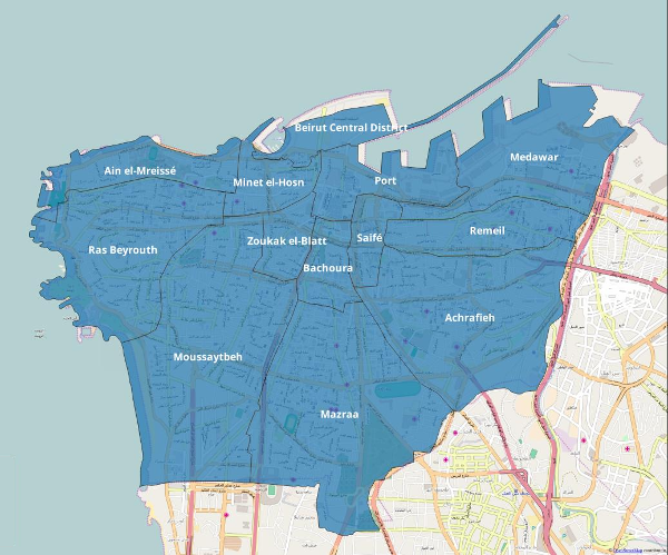
As seen in Figure 2, metropolitan Beirut is very approximately square, bounded by the Mediterranean Sea to the north and west and by the River Beirut to the east. Suburbs outside the administrative jurisdiction of the city extend to the east and south, reaching into the hills as part of Greater Beirut. The city comprises of 13 quarters (or quartiers); we consider 12 with Port and Central Business District (CBD) combined.1 The CBD is seen in the top middle. Other notable quarters are Ras Beirut to the west (the cosmopolitan university quarter); Achrafieh roughly east (a high-end quarter); and poorer areas in the south-west. Note that the blue overlay in the figure, showing the quartiers, has minor geographical differences from the underlying map due to geolocation offsets and to the most recent landfill activity. We use open-source GIS data from OpenStreetMap2 and the Lebanese Central Administration of Statistics (CAS)3.
Housing price index
Due to the lack of a housing price index in Lebanon or historical real estate prices for residential dwellings in Beirut, we estimate a two-stage least squares model to examine the housing market in Lebanon between 2000 and 2016. To do this we use the monthly average values for income, price, cost, and the lending rate.
The housing market in Lebanon had been in frenzy between 2008 and 2015, when prices had risen by more than 300% during that period. Then prices stalled in 2015 and onwards. The housing market stagnation since 2015 brought with it a heated debate among market participants and stakeholders fearing that the real estate market was experiencing a bubble. We use a structural framework of simultaneous equations of demand and supply to illustrate how price is determined by long term effects of income and cost by estimating a reduced-form model of equations for the endogenous variables such as quantity and price. Then we estimate a structural model by replacing the observed endogenous variables with their estimates from the first-stage regressions. Second, we allow for a partial adjustment process through which the actual price adjusts to its equilibrium level in each period. This adjustment process is equivalent to an auto-regressive (AR) process of price with income, cost and interest rate as exogenous variables.
We find that home price is well explained by the forces of demand (income) and supply (cost of construction and interest rate). However, price adjusts very slowly to its equilibrium level. The coefficient on the partial adjustment process for home price is 0.08. Income elasticity of demand is 0.98 which implies that for a percentage increase in income, home price increases by almost one percent. Price elasticity of demand is estimated by about -0.67 while interest elasticity of demand is -0.0134. Cost elasticity is estimated at about 3.162. Because cost elasticity is higher than either income or interest rate elasticities, we conclude that home price is largely driven by cost of construction. We also find a slow adjustment process in quantity of construction to its equilibrium level. The implied partial adjustment is given by 0.053. While cost of construction has relatively large impact on price, it is not a significant determinant of quantity. The price elasticity of supply is estimated by 1.212. The reported R-square in Table 3 implies that about 83% of variation in the demand for housing starts is explained by the price, income, and interest rate, while only 42% of the supply of housing starts is explained by price, cost, and interest. While demand is well explained by income, the supply of housing starts is largely affected by forces other than market dynamics (i.e., influx of refugees).
We next explain the estimation of a two-stage least squares model using the economic theory of demand and supply. This simple model helps explain the variation in the price of housing. This model also helps illustrate how price is determined by long-term effects of income and cost through a dynamic demand and supply mechanism by introducing a partial equilibrium adjustment in the housing market in Beirut.
In the first stage we estimate the following structural model in which the demand and supply sides are given respectively by:
| \[\begin{aligned} q_t &= \alpha_0 + \alpha_1 y_t + \alpha_2 p_t + \alpha_3 r_t + u_t \\ q_t &= \beta_0 + \beta_1 c_t + \beta_2 p_t + \beta_3 r_t + v_t \end{aligned}\] | \[(1)\] |
In equilibrium, by setting equations 1 and 1 equal, we obtain the reduced form equations for \(p^*_t\) and \(q_t\) as follows:
| \[\begin{aligned} p^*_t &= \lambda_0 + \lambda_1 y_t + \lambda_2 c_t + \lambda_3 r_t + \epsilon_t \\ q_t &= \gamma_0 + \gamma_1 y_t + \gamma_2 c_t + \gamma_3 r_t + \nu_t \end{aligned}\] | \[(2)\] |
In the second stage, we estimate the structural equations 1 and 1 using the predicted values for \(p_t\) derived in the first stage, i.e., \(p^*_t\) by equation 2. This gives respectively the demand and supply sides:
| \[\begin{aligned} q_t &= \delta_0 + \delta_1 y_t + \delta_2 p^*_t + \delta_3 r_t + v_t \\ q_t &= \mu_0 + \mu_1 c_t + \mu_2 p^*_t + \mu_3 r_t + \tau_t \end{aligned}\] | \[(3)\] |
Partial adjustment and analysis of the price index
The model described in equations 1– 3 assumes that the market for housing is in equilibrium at all time. However, in order to capture the dynamics of the housing market, particularly the rapid increase in housing price between 2007 and 2011, it is natural to allow for a partial adjustment process to reflect the gradual adjustment of price to transitory shocks such as influx of refugees. Through this adjustment process the actual price \(p_t\) adjusts to its equilibrium level \(p^*_t\) by a fraction \(\lambda\) of the difference \(p^*_t - p_t\) in each period, results in:
| \[\begin{aligned} p_t - p_{t-1} &= \lambda ( p^*_t - p_{t-1} ) \\ &= \lambda ( \lambda_0 + \lambda_1 y_t + \lambda_2 c_t + \lambda_3 r_t + \epsilon_t ) - \lambda p_{t-1} \\ p_t &= \lambda\lambda_0 + \lambda\lambda_1 y_t + \lambda\lambda_2 c_t + \lambda\lambda_3 r_t + (1-\lambda)p_{t-1} + \lambda\epsilon_t \\ &= \theta_0 + \theta_1 y_t + \theta_2 c_t + \theta_3 r_t + \theta_4 p_{t-1} + v_t \end{aligned}\] | \[(4)\] |
The parameter \(\lambda\) measures the effect of income, cost of construction, and interest rate on price. It captures the speed of adjustment between the desired price in time \(t\) (\(P^*\)) and the actual price \(P_{t-1}\) in time \(t-1\). Also, \(\lambda\) satisfies \(0<\lambda<1\). A \(\lambda=0\) implies that housing price is unable to adjust to its long-run equilibrium in response to changes in the explanatory variables.
The parameters of equation 4 can be calculated by estimating the AR(1) process in equation 4. Analogously, a partial adjustment process for the quantity of housing can be estimated by:
| \[\begin{aligned} q_t &= \gamma ( \gamma_0 + \gamma_1 y_t + \gamma_2 c_t + \gamma_3 r_t ) + (1-\gamma)q_{t-1} \end{aligned}\] | \[(5)\] |
The demand and supply equations 1 and 1 have their partial adjustment processes estimated in the second stage respectively as follows:
| \[\begin{aligned} q_t &= \alpha ( \alpha_0 + \alpha_1 y_t + \alpha_2 p^*_t + \alpha_3 r_t ) + (1-\alpha)q_{t-1} \\ q_t &= \beta ( \beta_0 + \beta_1 c_t + \beta_2 p^*_t + \beta_3 r_t ) + (1-\beta)q_{t-1} \end{aligned}\] | \[(6)\] |
| Variable | Mean | Std. Dev. | Min | Max |
|---|---|---|---|---|
| Price | 69448.19 | 28955.56 | 33445.80 | 126104.50 |
| ln(Price) | 11.06 | 0.42 | 10.42 | 11.74 |
| Income | 203.86 | 50.57 | 122.82 | 291.67 |
| ln(Income) | 5.29 | 0.25 | 4.79 | 5.71 |
| Cost | 92.97 | 10.47 | 74.50 | 105.30 |
| Change in Cost | 0.11 | 0.76 | -9.34 | 1.40 |
| ln(Cost) | 4.53 | 0.12 | 4.31 | 4.66 |
| Change in ln(Cost) | 0.00 | 0.01 | -0.12 | 0.01 |
| Interest rate | 10.73 | 3.62 | 6.89 | 18.51 |
| Quantity_sa | 792936.50 | 250248.60 | 464701.00 | 1267727.00 |
| ln(Quantity_sa) | 13.53 | 0.32 | 13.05 | 14.05 |
| Quantity_nsa | 808785.60 | 436054.80 | 111003.00 | 4835710.00 |
| ln(Quantity_nsa) | 13.50 | 0.45 | 11.62 | 15.39 |
| Price equation variable | Price | Price | Ln(Price) | Ln(Price) |
|---|---|---|---|---|
| Income | 424.0** | 49.53** | ||
| (33.17) | (14.85) | |||
| Cost of Construction | 1,211** | 61.06 | ||
| (219.6) | (81.50) | |||
| Interest Rate | 1,813** | 85.03 | 0.0233** | -0.000377 |
| (437.4) | (160.6) | (0.00639) | (0.00232) | |
| Price_lagged_AR(1) | 0.909** | |||
| (0.0238) | ||||
| ln(Income) | 0.918** | 0.0827* | ||
| (0.0934) | (0.0389) | |||
| ln(Cost) | 2.242** | 0.151 | ||
| (0.268) | (0.108) | |||
| ln(Price)_lagged_AR(1) | 0.912** | |||
| (0.0238) | ||||
| Constant | -149,063** | -9,973 | -4.191** | -0.135 |
| (20,284) | (7,979) | (1.014) | (0.372) | |
| Observations | 192 | 191 | 192 | 191 |
| R-squared | 0.925 | 0.992 | 0.933 | 0.992 |
| Quantity equation variable | Quantity | Quantity | Ln(Quantity) | Ln(Quantity) |
|---|---|---|---|---|
| Income | 3,713** | 145.0 | ||
| (353.5) | (137.3) | |||
| Cost of Construction | -7,336 | 1,620 | ||
| (11,729) | (3,605) | |||
| Interest Rate | -10,043* | -681.8 | -0.0172** | -0.000770 |
| (5,016) | (1,555) | (0.00604) | (0.00183) | |
| Quantity_lagged_AR(1) | 0.954** | |||
| (0.0225) | ||||
| ln(Income) | 0.916** | 0.0516 | ||
| (0.0853) | (0.0321) | |||
| ln(Cost) | -1.059 | 0.267 | ||
| (1.045) | (0.312) | |||
| ln(Quantity)_lagged_AR(1) | 0.947** | |||
| (0.0216) | ||||
| Constant | 144,309 | 15,376 | 8.874** | 0.460. |
| (122,283) | (37,643) | (0.510) | (0.244) | |
| Observations | 191 | 191 | 191 | 191 |
| R-squared | 0.770 | 0.978 | 0.827 | 0.985 |
Summary statistics for the variables reported in the model is reported in Table 1. The results of equations 2 and 4 are presented in Table 2 and those for equations 2 and 5 are presented in Table 3.
In the following analysis of elasticities that are derived from the model, we restrict the discussion to the results given by the log model, for the coefficients simply represent elasticities of the variables in question. Consequently, income elasticity as given by equation 2 in Table 2 is 0.918. In the AR(1) process given by equation 4 (column 4 of Table (2)), the coefficient on \(p_{t-1}\) is subtracted from one then the coefficient on income is divided by the result to obtain the elasticity measure that is comparable to the one given by equation 2. This results in income elasticity of 0.939.5 This indicates that for one percentage increase in income, housing price tends to increase by about 0.9 percent. Examining the quantity specification, equation 2, with its results reported in Table 3, the implied interest rate elasticity is -0.0138.6 That is, a 1 percent drop in interest rate, construction permits tend to increase by 0.0138%. However, the cost elasticity is 2.242, that is, a one percent increase in construction cost results in an increase in housing prices by 2.24 percent. This indicates that the surge of housing price over the period of study was more driven by cost increase than by variation in income. The coefficient on \(p_{t-1}\) in equation 4 is 0.912. The partial adjustment process indicates that the housing price adjusts very slowly to its equilibrium value (\(1 - 0.912 = 0.08\)). The fact that housing price is largely determined by income and construction costs, imply that the increase in housing price is well explained by the forces of supply and demand over the study period. However, the slow adjustment of price to its equilibrium level implies a widening wedge between supply and demand.
A similar pattern of adjustment for the quantity equation 5 as in the price equation above; the implied partial adjustment parameter in equation 5 is 0.046 for the linear equation and 0.053 for the log-linear equation. Income and interest rate are only significant in the baseline model without lags, with a sluggish response to cost. Income elasticity is in line with the one found in the price equation (0.916).
| Demand equation variables | Quantity | Quantity | Ln(Quantity) | Ln(Quantity) |
|---|---|---|---|---|
| Income | 3,863** | 126.8 | ||
| (347.5) | (140.5) | |||
| Price | -5.255* | 0.278 | ||
| (2.132) | (0.677) | |||
| Interest Rate | -8,514 \(\boldsymbol{\cdot}\) | -846.5 | -0.0134* | -0.00103 |
| (4,876) | (1,530) | (0.00580) | (0.00181) | |
| Quantity_lagged_AR(1) | 0.955** | |||
| (0.0229) | ||||
| ln(Income) | 0.979** | 0.0531 | ||
| (0.0829) | (0.0335) | |||
| ln(Price) | -0.670** | -0.0209 | ||
| (0.188) | (0.0598) | |||
| ln(Quantity)_lagged_AR(1) | 0.943** | |||
| (0.0222) | ||||
| Constant | 98,372 | 19,959 | 8.502** | 0.506* |
| (119,247) | (37,190) | (0.495) | (0.242) | |
| Observations | 191 | 191 | 191 | 191 |
| R-squared | 0.777 | 0.978 | 0.837 | 0.985 |
| Supply equation variables | Quantity | Quantity | Ln(Quantity) | Ln(Quantity) |
|---|---|---|---|---|
| Cost of Construction | -177.8 | 136.1 | ||
| (4,411) | (1,392) | |||
| Price | 6.786** | 0.237 | ||
| (1.167) | (0.397) | |||
| Interest Rate | -10,537 | -655.9 | -0.0466* | -0.0228 |
| (6,990) | (2,271) | (0.0211) | (0.0220) | |
| Quantity_lagged_AR(1) | 0.952** | |||
| (0.0228) | ||||
| ln(Cost) | -3.162* | -1.969 | ||
| (1.437) | (1.463) | |||
| ln(Price) | 1.212** | 0.764* | ||
| (0.323) | (0.352) | |||
| ln(Quantity)_lagged_AR(1) | 0.418* | |||
| (0.190) | ||||
| Constant | 451,447 | 17,460 | 14.90** | 8.546* |
| (406,581) | (129,592) | (3.853) | (4.266) | |
| Observations | 192 | 191 | 192 | 191 |
| R-squared | 0.778 | 0.978 | 0.421 | 0.426 |
| Demand | Supply | |
|---|---|---|
| Income elasticity | 0.979 | – |
| Cost elasticity | – | -3.162 |
| Price elasticity | -0.670 | 1.212 |
| Interest elasticity | -0.0106 | -0.0369 |
The results of the structural model of equations 3 and 3 and equations 6 and 6 are reported in Tables 4 and 5 respectively. A summary of elasticity measures is reported in Table 6.
Mapping prices to city quarters
The housing price index derived above pertains to the whole city. In order to derive average housing price per city quarter from \(p^*_t\), we triangulate two data sources: property price snapshots reported in the real estate trade press, and property maintenance levels. The former we describe next; the latter we discuss in the following sub-section.
We collected data on property prices at the street or neighbourhood levels, from the real estate press. We consolidated the observations under the 12 cadastral areas for the period 2008–2015. For example, we obtained about 20 different prices for each quarter every month for both land and housing. We take the average of each type of prices and calculate the percentage change in price. In order to assure continuity, the percentage change is used to fill the gaps to construct a unified index for housing. When a price of housing is missing for a particular month, we used the percentage change in the price of land for the same month to calculate the price of housing and vice versa. This process is iterated for the 12 cadastral areas.
Property maintenance index
Besides prices, the RGT is predicated on the maintenance conditions of properties, to be able to compute their rent gaps. In order to obtain data about the current maintenance conditions in Beirut, we undertook a survey in summer 2017. In total 1,440 residential dwellings were surveyed. In order to understand the history of the buildings and neighbourhoods, the survey teams also interviewed the doorman/janitor of apartment buildings, and spoke with the local municipal registrar.
Since data about neither current nor historical conditions of buildings is available, other than our survey, we projected backwards from the survey results in order to estimate a historical index of maintenance levels. This projection was performed based on expert opinion about the quarters at aggregate level, from real estate agents and municipal registrars. For buildings constructed or refurbished within our time period of interest, we assume their initial maintenance condition is the highest possible.
Population data
With demographics of Lebanon being a delicate matter for sectarian and political reasons (Hägerdal 2019), estimates circa 2009 put the Lebanese population living in the country at around 4 million7 , besides approximately 0.5 million long-term Palestine refugees from 1948 and later. By 2015, the UN recorded more than 1 million official refugees from Syria; including undocumented refugees and those who have emigrated, e.g., to Europe, through Lebanon, the estimates are as high as 2 million, i.e., up to 50% of the national population.
We adopt annual total population estimates and projections from the UN (United Nations Population Division 2019), and ethnicity distribution from commonly-cited estimates (Lebanese Information Center 2013; US Central Intelligence Agency 2019); religion of each ethnicity is set accordingly. Because of the unique living and mobility factors concerning Palestinian refugees, we exclude this population from our model.
Sources including World Bank figures8 and aggregate voter registration records9 provide estimates of the total population of Beirut. In order to obtain population totals per city quarter, we project proportionally to the most recent CAS population density figures and the quarter’s size. A priori we assume that the demographic mix is the same in each quarter, except for where expert opinion advised that certain areas are more segregated on sectarian lines.
Locations: City structure, economic dynamics
The city is represented in the model as a geo-located set of locations; each location is situated in one administrative district. For the case of Beirut, these districts are the quarters. Each location comprises of a set of buildings, streets, and other urban features. We model these together, characterising the location by a value, \(V\), a maintenance level (or repair state), \(r\), and a population count, \(N\). For each location, we initialize these variables within a small random window around the data values for the quarter, obtained as described in the previous subsection. Repair states are normalized a \([0,1]\) scale, while the population count within each quarter is proportional relative to the simulated city population, as described in the next subsection.
We choose the time unit of the simulation to be one calendar month. This is because, first, economic and migration data is available at resolution of at best one month. Second, it is in line with prior studies of the rent-gap theory using ABM (Picascia et al. 2015).
Locations can be occupied by zero or more residents, up to specified population limits. If the population exceeds the limit—or if the location’s condition falls too low (\(r \le 0.15\))—then the location is deemed to be a slum. Dwellings progressively decay in their condition by a factor \(d=0.0012\) assuming that, if unmaintained, a location goes from 1 (perfect) to 0 (inhabitable) in 70 years (since 1 simulation step = 1 month). In order to match the theoretical assumption of a decline in property price over time, we set the value of the dwelling as decreasing by a depreciation factor of 0.02 / year, as proposed by Diappi & Bolchi (2006). We also assume that in case of prolonged emptiness of the dwelling (beyond 6 months) both decay and depreciation factors are increased by 20%. These factors also increase for over-populated locations.
The model considers investment in housing renovation and redevelopment as the fundamental economic force. The capital parameter, \(K\), represents the maximum number of locations that can be redeveloped in the current economic climate, expressed as a fraction of the total number of locations of the city, following Diappi & Bolchi (2006).
In line with Picascia (Picascia 2015; Picascia & Yorke-Smith 2017), the selection of locations where investment occurs is carried out deterministically, based on the value gap of a location with the neighbouring properties, in accordance with the RGT. The relevant value gaps are determined in accordance with the neighbourhood effect: the principle that the amount of rent or the sale value attainable by a given location is always bounded by the characteristics and the desirability of the area where the property is located. We set the new value \(V'\) of a redeveloped property \(x\) at the average of the surrounding locations in a radius of 2, plus 15% (representing a premium for a newly-restored property): \(V'_{x} = 1.15 * \textrm{avg}(V_\text{radius2})\label{eq:pricegap}\). The value gap for location \(x\) will be \(G_{x}=V'_{x}-(V_{x}+C_r)\), or 0 if \(G_{x}<0\); \(C_r\) is the cost of removing the present residents if the location is occupied. The cost of removing a refugee (0.01) is lower than for a non-refugee (0.05), but there can be more refugees in a location (maximum population 6) than non-refugees (maximum 3). Once a location is selected for investment, its value is set at \(V'_{x}\) and its repair state is set at \(r=0.95\).
For the case of Beirut, we also model government policy which mandates properties in the CBD be maintained to a minimum standard and to have a lower maximum population than other quarters.
Table 7 summarises the variables associated with location.
| Name | Type/Range | Description |
|---|---|---|
r |
float, {0,1} | maintenance state |
V |
float, {0,1} | value (at market rates) |
G |
float, {0,1} | value-gap: difference with neighbourhood value |
d |
integer | distance from the centre of city |
te |
integer | time empty (months) |
| o | boolean | occupied? |
Agents: Residential mobility, cultural exchange
Agents in the model represent individuals or households. Each agent is endowed with an income level, \(i\), a mobility propensity, \(m\), and a tuple that represents its cultural configuration, including ethnicity and religion (Table 8). The agent’s income level is strongly correlated with its ethnicity, reflecting the stratification of highly unequal Lebanese society; incomes represent the highest price that the agent is able to pay for the right of residing in a property. Agents of most ethnicities, refuges excluded, are able to apply for credit that multiplies their purchasing power. Agents of Lebanese or Arab nationalities, refugees excluded, can own property. If the property is owned, its condition depreciates more slowly. Owners have a reduced propensity to move compared to renters, and are not forced to leave their current (owned) residence if rental prices increase.
| Name | Type/Range | Description |
|---|---|---|
m |
float, {0,1} | mobility propensity |
c |
list t=10, v=4 | culture: memetic code |
i |
float, {0,1} | income level |
d |
float, {0,1} | cognitive dissonance level |
th |
integer | time here: months spent in the current location |
The agent’s culture is modelled as a tuple of \(t\) multi-valued traits, inspired by Axelrod (1997) and originally applied to the urban context by Benenson (1998). Each cultural trait can assume \(v\) variations, giving rise to \(v^{t}\) possible individual combinations. The semantics of traits are emergent, with the exception of the first two traits to which we assign reserved meaning. First, ethnicity may be one of five values: Lebanese, (Arab) refugee, affluent Arab non-refugee, professional non-Arab (e.g., from Europe), and working class non-Arab (e.g., domestic servants from south-east Asia); ethnicity does not change. The second reserved trait models religion, which may be one of five values: Christian (various sects), Druze, Shi’a Muslim, Sunni Muslim, or other; religion has a small possibility of changing according to the process described next. Initial values for ethnicity and religion are assigned randomly according to the data described earlier. Initial income is set according to the estimated Gini coefficient of Lebanon, and reported mean incomes of Lebanese and non-Lebanese (United Nations Development Programme 2008; United Nations High Commissioner for Refugees 2016, 2017).
The model allows traits, excluding ethnicity, to change according to the influence of other agents. Cultural influence is localised: agents that have been neighbours for more than six consecutive months are likely to interact and exchange traits, thus rendering the respective cultural tuples more similar (Picascia 2015). At the same time a cultural ‘cognitive dissonance’ effect is at work, implementing Portugali’s concept of spatial cognitive dissonance (Portugali 2004, 2011). Similarity between two agents is defined as the proportion of traits they share. Agents who spend more than six months surrounded by neighbours with commonly-held traits increase their mobility propensity each subsequent month. The mobility propensity attribute represents the probability that an agent will abandon the currently-occupied location in the subsequent month. Mobility propensity is affected by the conditions of the currently occupied dwelling and the cognitive dissonance level. A special circumstance is when the price of the dwelling currently occupied exceeds the agent’s income \(i\). This represents an excessive rent increase, unsustainable by the agent.
The process of finding a new location is bounded by the agent’s income: a new dwelling has to be affordable (\(V\leq i * \textit{credit}\)) and in relatively good condition (at a minimum, not a slum); and closer to the CBD is preferable (since Beirut is a monocentric city). If no affordable and available location is to be found, the agent is forced to leave the city. The exception is refugees, who will consider moving to a location of poor condition or of high population, and only leave the city if even no slum is to be found.
Results and Analysis
Our specific research questions concern the effects of mass refugee inflow into Lebanon. At the time the research was performed, the country hosted the most refugees of any country in relation to its population (United Nations High Commissioner for Refugees 2016). Profound consequences of such a large influx of population in a short time period include social, economic, security, and political aspects (Cherri et al. 2016). Our research questions focus on the first two aspects—i.e., social and economic—as follows:
- Can qualitative effects of the refugee influx be seen?
- What effects does a sudden large influx of low income people have on the economic housing cycle?
- What public or Non-Governmental Organization intervention actions might be effective?
We measure a number of output variables from the simulation, including location condition and prices, population income and cultural traits, occupancy rates and mobility, neighbourhood allure and cultural mix, and immigration and emigration counts. In particular, for the experiments reported below, we recorded:
- % of slum locations (\(r \le 0.15\)),
- % of well-maintained locations (\(r > 0.5\)),
- % of over-populated locations (\(N > 3\)),
- median price of all locations,
- median income of all people,
- the quarter with the highest median price,
- the quarter with largest number of refugees, and
- % of Lebanese, refugees, or another ethnicity.
We first sought to validate the model, and then conducted three exploratory experiments directed towards our research questions. Simulation parameters were set following our preliminary work (Picascia & Yorke-Smith 2017), which in particular explored the effect of capital \(K\) and the type of rent gap computation; additional parameters settings are reported below.
Validation
In order to investigate the validity of the model, we assessed whether the simulation produces at a qualitative level results similar to the real-world situation at a later point in time, given as input the real-world situation at an earlier point in time. We do not expect this historical replay (Van Dam et al. 2013) to be exact, given the fidelity of the simulation, and the range of exogenous factors (such as global economic conditions, domestic political events, and changes in property legislation) outside its scope.
We note that the core ABM was validated by this kind of historical reproduction, for the British cities of Manchester (Picascia 2015) and London [unpublished]. Although post-industrial Britain and contemporary Lebanon have obvious economic and societal differences, the underlying economic model, the RGT, is argued to be applicable in all housing markets in capitalist economies, since the fundamental processes described by the theory—profit-driven investment in house building—are not too dissimilar across different property markets. The previous validation suggests that the model captures at least some of the dynamics involved in such process. More substantial differences between property markets are to be found in the distribution of wealth, income, and tenure, in government policy, in the amount of investment capital available in the economy. The model allows us to vary these factors and study their effects.
We identify 2009 as the starting year for the validation. This year is well after the period of the Lebanese Civil War (approx.–1990) and the following reconstruction, and the short 2006 war and immediate reconstruction. It is prior to the influx of refugees from the Syrian Civil War (commencing 2011). As described earlier, agent demographics are initially set proportional to estimated figures prior to the influx of Syrian refugees, which became voluminous in early 2013. As noted, we do not consider other refugee populations, such as those of Palestinian origin already in Lebanon.
Thus we commence the simulation in 2009 with the housing prices, maintenance conditions, and population estimates for that year. We input the pattern of refugee influx from mid-2012 until mid-2015, when the Lebanese government changed entry regulations and other policies, discouraging refugees, and when the government also prohibited the UNHCR from officially registering any more Syrians in Lebanon as refugees. We compare the output of the simulation in 2015 with the estimates of real-world values at the end of that year in terms of relative district price changes.
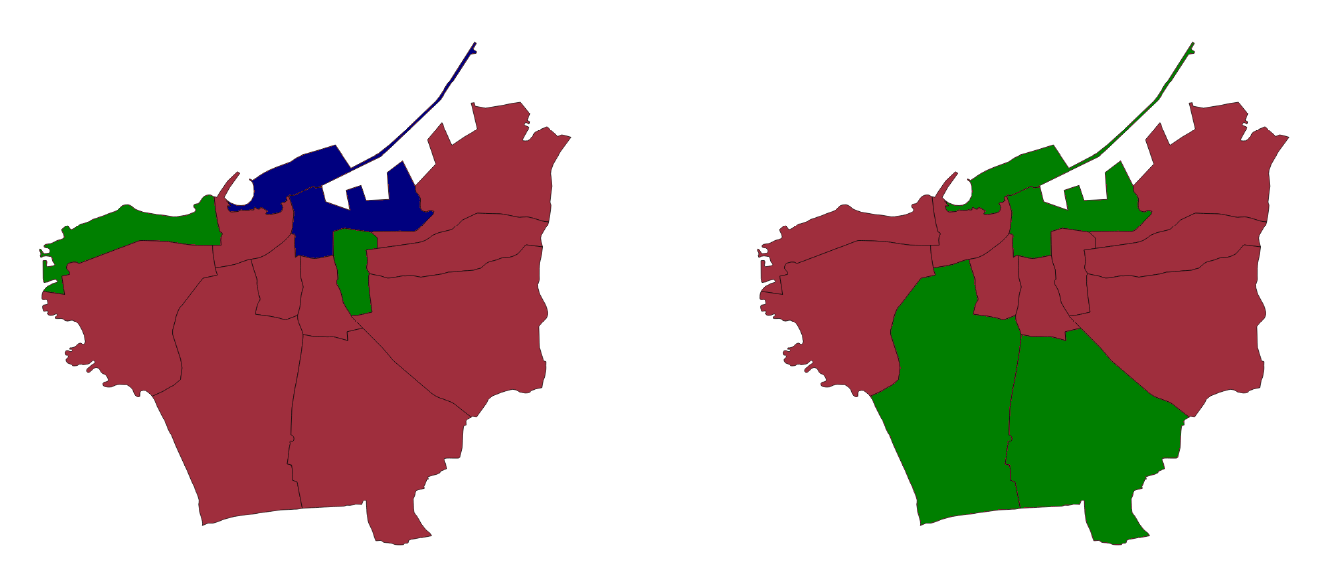
Figure 3 shows the simulation results (left) versus the actual prices (right). Due to the abstraction of the RGT model and the fidelity of the data, the simulation is not intended for quantitative forecasting. At a qualitative level, however, we see the simulation reproduces the general upward trend of prices. It correctly identifies that two central districts do not have price increases, albeit suggesting (small) price declines rather than steady prices.
Sensitivity Analysis
We perform an initial multi-variate statistical analysis. The purpose is to gain a broad view of which input factors are significant for which output variables. The analysis looks at the end-point in time: it does not reveal the evolution of the variables over the duration of the simulation. We examine the latter below.
Table 9 reports the results of a Type I MANOVA between the numerical output variables and three input factors. The factors are the capital, \(K\) (levels: \(0.015\), \(0.025\), \(0.035\), \(0.045\)), the migration treatment (levels: none, some refugees, more refugees, ongoing) and the intervention treatment (levels: none, regeneration, slum improvements). The latter two variables are described in more detail below, in the specific experiments.
| Variable | % slums | % maintained | % overcrowded | price | income | % Lebanese | % refugees | % others |
|---|---|---|---|---|---|---|---|---|
| K | *** | *** | *** | *** | *** | * | ||
| Migration | *** | *** | *** | *** | *** | *** | ||
| Intervention | *** | *** | *** | *** | ** | |||
| K:Migration | *** | *** | ** | *** | ** | *** | ||
| K:Intervention | *** | *** | *** | *** | ||||
| Migration:Intervention | *** | *** | *** | *** | ** | *** |
For the first four outputs, all three inputs are highly significant (\(p < 0.001\)), and for the fifth output, income, only variable intervention is slightly less significant (\(p < 0.01\)). The interaction effects are also significant, although less for ‘% overcrowded’, and not for \(K\) and migration together on income. By contrast, for the demographics outputs—the last three output variables—there is no found correlation, except for input migration on output ‘% others’.
In order to investigate further the consequences of mass refugee inflow, we next perform three experiments which study further the two treatments. In order to see the effects in the context of the economic cycle, we run the simulation for 600 months, simulating 50 years.
Experiment 1: Impact of Refugee Influx
In the first experiment we examine scenario ‘(Some) Refugees’. We simulate a refugee influx beginning at month 90 and continuing until month 180. The immigration rate for refugees, \(0.15\), is much higher than the rate for non-refugees, \(0.02\); the emigration rates are \(0.012\) and \(0.019\) respectively. These rates reflect that after refugees arrive in Lebanon, many settle for an extended period of time before obtaining access to a country of asylum, returning to their own country (e.g., if the situation improves), travelling to a third country, or becoming de facto permanent residents in Lebanon.10 We also examine an extended influx continuing until month 270: scenario ‘More refugees’.
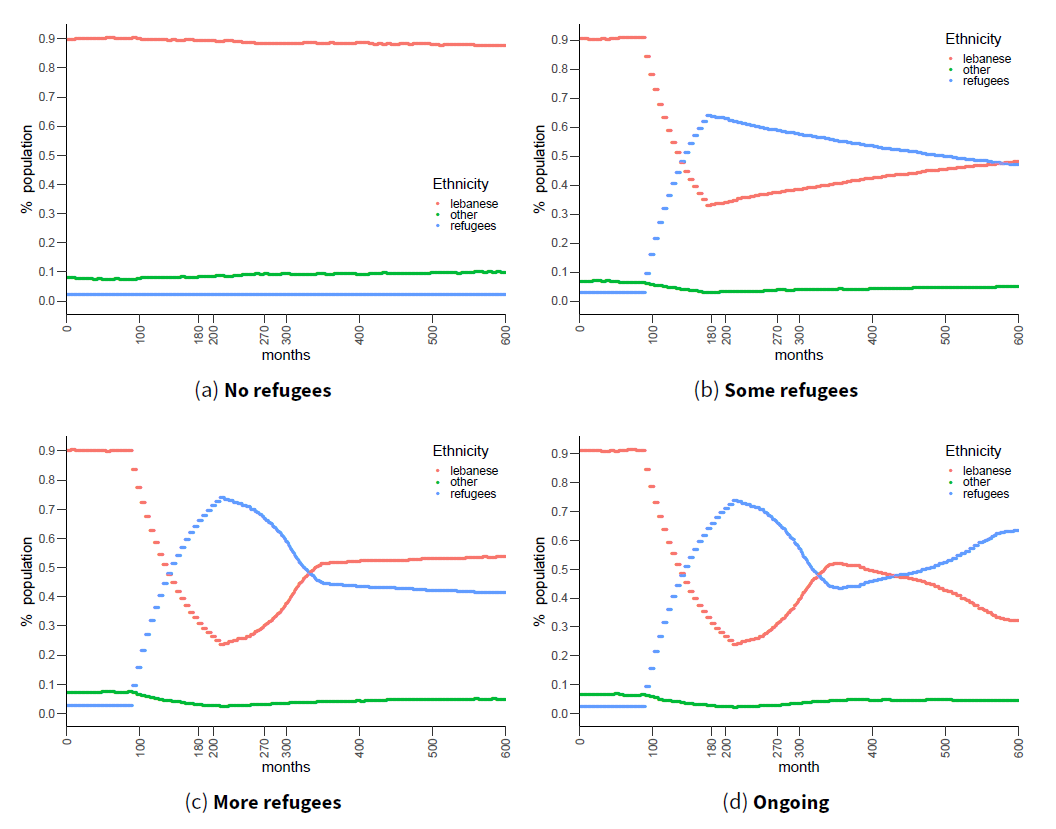
Figure 4 shows the evolution of the city population over time under four scenarios: no refugees (i.e., refugee immigration rate is the same as other populations: there is no influx), the two refugee scenarios explained above, and also scenario ‘Ongoing’ examined below in the second experiment. We partition the population into three groups: Lebanese (red line), refugees (blue line) and all other demographics (green line). The figure shows the percentage division of the total population into these three groups. Capital \(K = 0.025\). In the top row, the difference between none and some refugees is seen: the influx between \(t=90\) and \(180\) causes substantial displacement of the Lebanese population by refugees, which is slowly reversed as refugees migrate further.
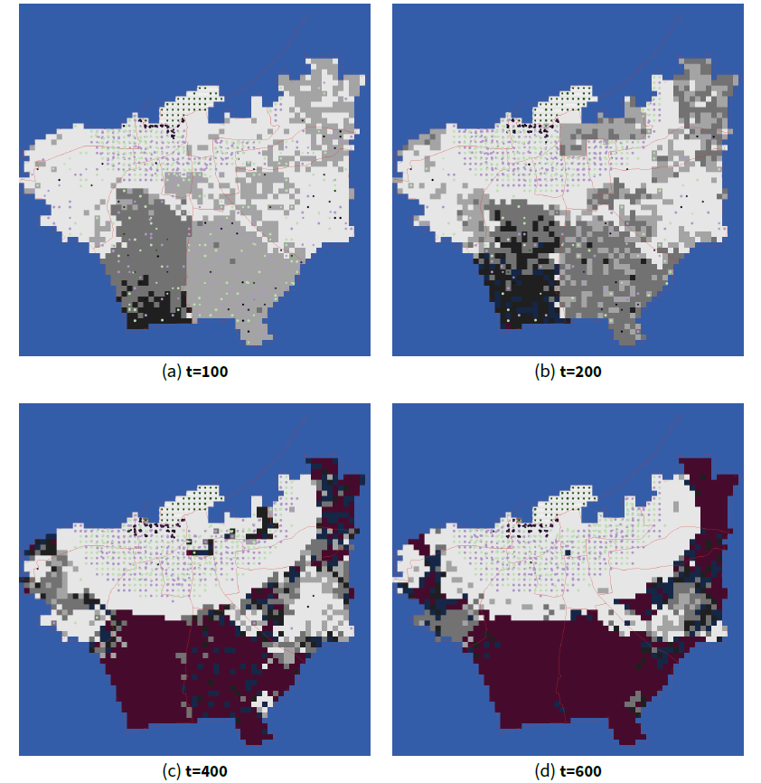
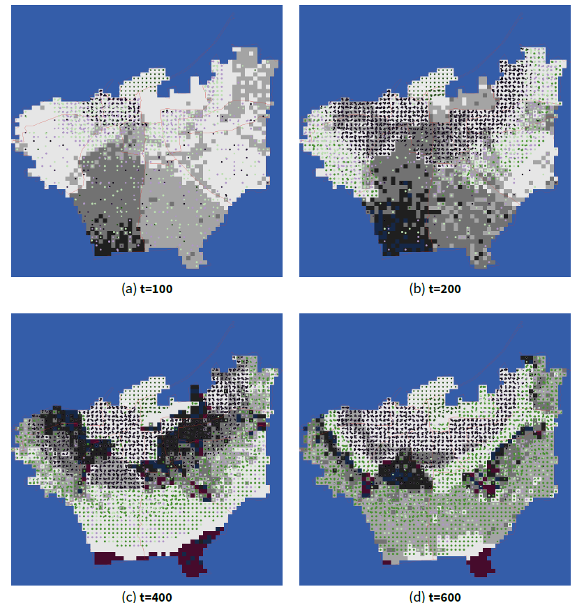
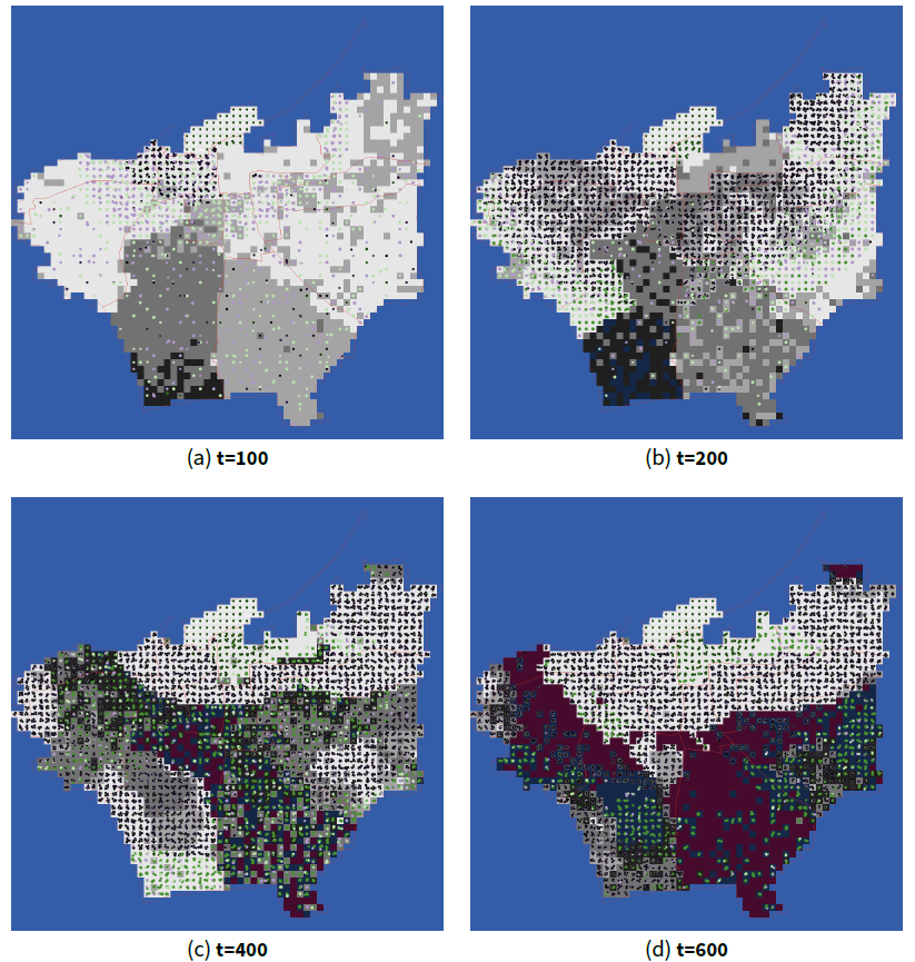
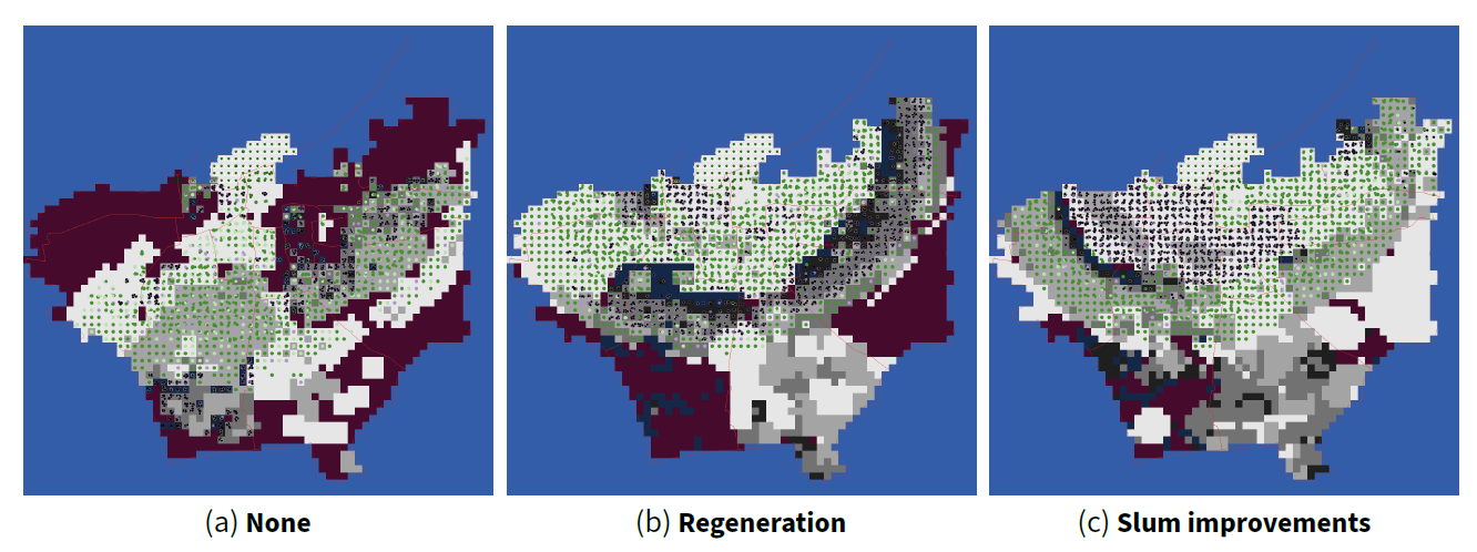
Figures 5– 7 show typical longitudinal views of the city locations under three of the scenarios: top, no refugees; middle, refugee influx (i.e., ‘Some refugees’); bottom, ongoing refugee influx. Again capital \(K = 0.025\). City locations are shaded according to their condition. The darker the shade of grey, the lower the condition of the location. Locations which have reached slum condition (\(r \le 0.15\)) are coloured dark blue; locations which have become inhabitable (\(r = 0\)), dark purple. Agents are depicted by colour, shape, and size. Colour denotes income: darker green indicates highest quintile, brighter green above average, brighter purple below average, and darker purple bottom quintile. Shape denotes the ethnicity of the agent: Lebanese are shown as filled circles, refugees as hollow circles, affluent Arab non-refugees as smiling faces, professional non-Arab as flat faces, and working class non-Arab as sad faces. Size denotes ownership: owners appear larger than non-owners.
First, notice some decline and regeneration—the economic cycle—affecting different city locations in the no-refugees case (top row). For example, district Port (top centre), starts with relatively high condition, has decayed to medium condition by \(t=200\), and has regenerated to a good condition by \(t=600\). Second, comparing Figures 5 and 6, interestingly we see that the number of slum locations is greater without the presence of refugees in this particular run of the simulation. At this level of capital, it seems that the economy lacks the ability to regenerate areas farther from the CBD once they fall into disrepair (what we might call the ‘Detroit effect’ (Downs 2011)). With the presence of refugees, the number of over-populated locations is reduced. There presence boosts demand for lower-price housing and ensures landlords do not have vacant properties. Since there are fewer slum locations, there is more habitable properties and less over-crowding overall. Third, we observe a trend for segregation between refugee and non-refugee populations, emerging from the combination of economic and cultural factors.
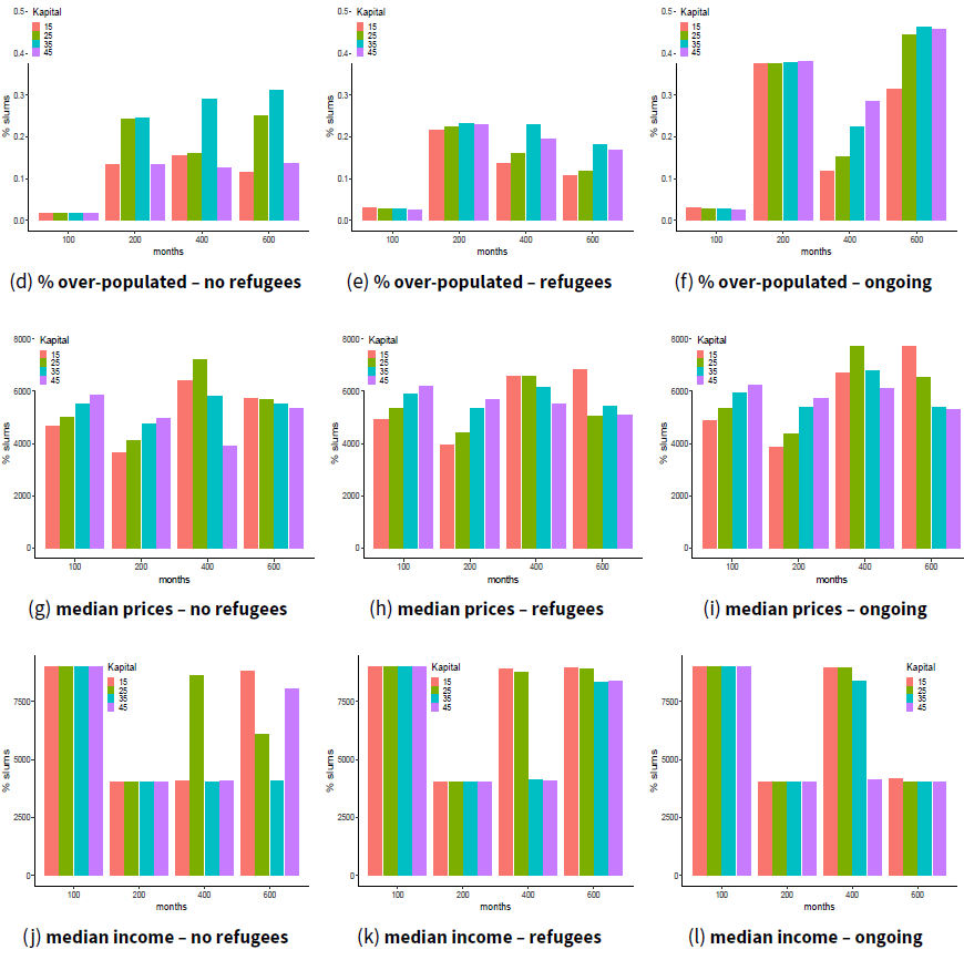
In order to explore further the impact of the refugee influx, we performed 100 iterations (with random seed) for each of four levels of capital \(K\), and computed output variables shown in Figure 8 and Table 10. The top row of the figure shows the proportion of slum locations under no refugee (left) and refugee (centre) conditions. In each graph, we examine four levels of \(K\), plotting the output variable over time for each level. At low levels of \(K\), the ability of owners to regenerate dwellings is limited. As expected, in both with- and without-refugee conditions, at the lowest levels of \(K\), the proportion of slums increases.
From an economic theory perspective, the presence of refugees reduces the profitability of redevelopment in two ways: (1) when a location is occupied there is the resident removal cost \(C_r\) to be paid in order to redevelop it; and (2) since in the model the prices of non-empty locations decline more slowly than empty ones, price-gaps with higher priced neighbouring properties also widen more slowly. This last effect is more pronounced when a large contiguous area is under-maintained but occupied: there is less incentive for private capital to invest and regenerate the locations, so the area keeps declining. On the other hand, the presence of refugees implies increased demand for property. If refugees take the lower-priced properties, this has potential to displace residents with higher income into higher priced properties, potentially increasing the incentive to redevelop and rent the property towards this demand.
Table 10 shows (top three rows) that in the long run the impact of refugees on the amount of under-maintained locations is positive (fewer slums). The table averages across the values of \(K\) at month 600, averaged over the 100 runs of the simulation in each migration scenario. From Figure 8, we know that the metrics at this time are not the whole story. Nonetheless, the normal economic cycle of investment is capable of absorbing the shock of the mass refugee influx that ends at month 180 or indeed that continues to month 270, and by month 600 the % slums is reduced. This is not the case when we test an ongoing refugee influx in Experiment 2 below. For a limited influx, an explanation could be that in the very long run refugees will have left (e.g., gone back to their place of origin) or (partially) will have integrated in the host society and improve their socio-economic status and are able to move out of slums. The increasing demand motivates a larger rent-gap, and thus the redevelopment of poor maintenance properties.
The second row of Figure 8 shows the proportion of over-populated locations. As with % slums, the % overcrowded is lower in the long term in scenarios with limited refugee influx. We also observe that refugees have a more even effect on overcrowding (than on slums): narrowing the observed differences across different levels of capital, compared to the no refugees case.
The third row of Figure 8 shows the median prices across the whole city. These snapshots at four points in time do not show how the distribution of prices between districts changes over time (Figures 5– 7). Prices overall are comparable when refugees are present, except when capital is low in the economy. The overall increased demand for housing pushes up prices for habitable locations, and the market sustains itself despite the changing populations.
The fourth row of Figure 8 shows the median income. Interestingly, overall median income is higher when refugees have been present (Table 10, last column). The differences observed between ‘No refugees’ and ‘Some refugees’ scenarios can be attributed to the mix of agent types in the population (Figure 4). Further, refugees imply an increase in aggregate demand for goods and services, and cash inflow from NGOs such as UNHCR.
| Migration | % slums | % overcrowded | price | income |
|---|---|---|---|---|
| No refugees | 0.41 | 0.20 | 5560 | 6750 |
| (Some) refugees | 0.28 | 0.14 | 5600 | 8620 |
| More refugees | 0.27 | 0.13 | 5700 | 8900 |
| Ongoing | 0.51 | 0.42 | 6240 | 4070 |
Experiment 2: Impact of Ongoing Migration
When the flow of refugees does not cease (scenario ‘Ongoing’), the effects observed in Experiment 1 are further pronounced and new effects are seen: the right-most column of Figure 8 and the bottom row of Table 10.
Visually, Figure 7 shows widespread highly-populated, slum, or uninhabitable locations by \(t=400\). Although the economic cycle continues—observe the regeneration of the south-west between \(t=200\) and \(400\)— in contrast to the second row of the figure, the economy is overwhelmed by the ongoing influx, and by \(t=600\) locations are falling into permanent disrepair. The shock of the influx overwhelms the system and the % slums climbs.
The decline in property conditions and the spread of locations in permanent disrepair causes several effects. First, as one might expect, other quarters become densely populated at all levels of capital. Second, non-refugees leave the city in the longer term, as they can find no affordable place of reasonable condition with space (Figure 4). This causes also the median income to fall, as seen in Figure 8(l). Third, refugees leave the city when they too can find no place, despite their willingness to accept poorer conditions and greater population density. They can be replaced by returning citizens. Those locations which are inhabitable find higher prices due to lack of supply alternatives for housing.
Experiment 3: Impact of Interventions
We consider two types of interventions in the housing market. First, top-down government intervention to regenerate a location of poor condition. This periodic action, every six months with our baseline parameter settings, seeks out one of the locations of lowest condition (it need not have decayed to slum condition), lifts its condition to \(r=0.95\) and raises its price correspondingly, and lifts similarly the condition of the immediately surrounding locations.
The second type of intervention targets locations that have reached slum condition. It makes specific improvements to one such location, to a condition \(r=0.5\), and it can occur on a monthly basis rather than bi-annually.
While the first type of intervention has not occurred in Beirut, there is a legal framework for it were there sufficient funds and political consensus (UN HABITAT 2014). In contrast, the second type has occurred in recent years, funded by donor countries or NGOs.
Figure 9 and Table 11 depict the effect of no intervention, regeneration, and targeted slum improvements. From left to right, Figure 9 gives snapshots from a single simulation run of these intervention policies (i.e., one run for each), at month 600 with the level of capital \(K = 0.035\). Similar to Table 10, Table 11 shows the average over 100 runs of each policy, again at month 600 and averaged over the values of \(K\).
| Intervention | % slums | % overcrowded | price | income |
|---|---|---|---|---|
| None | 0.28 | 0.14 | 5600 | 8620 |
| Regeneration | 0.21 | 0.16 | 5170 | 8470 |
| Slum improvements | 0.27 | 0.15 | 5580 | 8530 |
The greatest contrast is seen between some kind of intervention and none at all. Both top-down neighbourhood regeneration actions and more frequent and targeted slum improvements counteract the dampening effect of the refugee shock on the city’s housing market. While the top-down regeneration makes best reduction of % slums, the more frequent micro-interventions are better able to break out neighbourhood ‘clusters’ of poor condition dwellings. Top-down regeneration reduces the median price, which has both pros and cons from an economic perspective. More regeneration of properties adds to the supply of housing which pushes the price down. This is a supply side-induced increase in housing which dumps the price, unlike the demand-side induced policies which have the opposite effect on price.
The suggestion opened for future study is that interventions can have value in sustaining the urban economy and population, mitigating the impact of the shock, and most importantly, improving the living condition of the poorest residents.
Discussion and Future Work
Our motivation comes from the sizeable contemporary international migrations affecting (from 2010) notably countries in West Asia and Europe. Our objective is to use ABM to explore the effect of migrant inflows on urban dynamics, and eventually to develop tools to aid policy makers with questions about the urban environment. This objective gains importance in the contemporary context: "the Syrian refugee emergency…reinforced a growing awareness in the international community of the need to address the situation of refugees in urban contexts" (Crisp et al. 2013).
In this article we presented a calibrated simulation model of a West Asian capital city that has experienced a significant refugee influx in the last decade. Our model extends earlier works by including designated cultural traits, property ownership (rather than a pure rental market), emigration, and refugees; and it goes well beyond the most recent related work (Picascia & Yorke-Smith 2017) by using data for population, housing prices, and property conditions. Our contribution includes devising indices for housing prices and other factors. The result is the first (to our knowledge) validated ABM of the Beirut housing market and the first such use of ABM to study urban dynamics in the context of migration.
Outcomes from the model exhibit that refugees have some surprising impacts on prices and slum locations, as well as impacting population density. Their presence can cause price spikes and invigorate or dampen the natural economic cycle, which continues nonetheless with waves of decay and regeneration. We observed a further interesting effect depending on the capital in the economy and the rate of mobility, whereupon excessive shock of refugees—and in particular ongoing migration to the city—can render large sections of quarters uninhabitable, causing parts of both refugee and non-refugee populations to emigrate from the city.
Our next step is to expand the geographic scope of the model from the city boundaries of Beirut to include the sub- and peri-urban areas of Greater Beirut. The importance of modelling the larger catchment area is that nearly half the population of Lebanon lives within the greater metropolitan area, with profound effects on property prices, mobility, and traffic (Fawaz & Sabah 2015; US Central Intelligence Agency 2019).
A weakness of an analytic approach, whether equation-based or agent-based modelling, or other, is the inability to account for out-of-expectation exogenous shocks to the system. For instance, in Beirut in 2019 the long-brewing debt burden led to non-partisan protests, forcing a caretaker technocrat government. Currency devaluation and COVID-19 epidemic caused refugees to leave Beirut and return to Syria where the situation was better (Ward & Lewis 2020).
Looking ahead, since significant migrations from West Asia (and other regions) have been absorbed not only by regional countries such as Lebanon, but also by developed countries that accept asylum seekers, we see value in applying our model to cities in Europe such as in Germany (Gore et al. 2019; Hatton 2017). An interesting research approach would be to further use ABM to study the migration decision-making of displaced persons (Collins & Frydenlund 2016; Hébert et al. 2018). They must decide whether to stay in a (precarious) intermediate country such as Lebanon with the hope of official migration via the UN to, e.g., Canada; return to the Syria if the situation there improves relative to the intermediate country; relocate to another intermediate country, e.g., Turkey; or attempt illegal migration to, e.g., Germany.
Model Documentation
The model has been built using NetLogo. The code is available at: https://www.doi.org/10.4121/13033154.Acknowledgements
For their constructive comments, we thank the anonymous reviewers of JASSS, and of the ABMUS’16, ’17 and ’18 workshops, and of AAMAS’18. We thank Joseph Bechara, Bruce Edmonds, Mona Fawaz, Lea Halabi, Alison Heppenstall, and our student assistants. This work was partially funded by the University Research Board of the American University of Beirut under grant number 103183, by the Lebanese National Council for Scientific Research (CNRS-L) under grant number 103290, by the Research Councils UK / Medical Research Council (MRC) under grant numbers MC_UU_12017/10 and MC_UU_12017/14, and by TAILOR, a project funded by EU Horizon 2020 research and innovation programme under grant number 952215.Notes
- The historical quartier of Port is split into Port and CBD. The long tail reaching into the sea is the breakwater of the Port of Beirut.
- www.openstreetmap.org.
- www.cas.gov.lb.
- During the period of study, and indeed until 2019, the Lebanese Pound was fixed in exchange rate to the US dollar.
- This is obtained from Table 2 as follows: \(1-0.912=0.08\), then \(0.0827/0.088=0.939\).
- Because interest rate is the only variable that is used in level rather than in log; therefore, its elasticity is measured by:
Consequently, is:\[\ln{P} = \lambda r \implies P = \exp(\lambda r) \implies \frac{\partial P}{\partial r} = \exp(\lambda r) \times \lambda = \exp((-0.0172)(10.73)) \times (-0.0172) = -0.0143.\] \[(7)\] \[\frac{\partial P}{\partial r} \times \frac{r}{P} = (-0.0143)(\frac{10.73}{11.06}) = -0.01387.\] \[(8)\] - The Lebanese diaspora is estimated to be 8–14 million (Lebanese Information Center 2013). They influence the housing market by ownership for investment or, in some cases, planned future repatriation. We treat these as exogenous factors and exclude them from our model.
- data.worldbank.org.
- www.lebanon-elections.org.
- Legal permanent residency is not permitted (Government of Lebanon & United Nations 2017).
Appendix: Acronyms
| BDI | Belief-Desire-Intention |
| CBD | central business district |
| MANOVA | multivariate analysis of variance |
| NGO | non-government organisation |
| RGT | rent-gap theory |
| UNHCR | United Nations High Commissioner for Refugees |
References
AHWASH, S. (2018). On Lebanon’s corruption. Al-Nahar: https://en.annahar.com/article/915724-on-lebanons-corruption.
ANDERSON, J., Chaturvedi, A., & Cibulskis, M. (2007). Simulation tools for developing policies for complex systems: Modeling the health and safety of refugee communities. Health Care Management Science Volume, 10, 331–339. [doi:10.1007/s10729-007-9030-y]
AXELROD, R. (1997). The Dissemination of Culture: A Model with Local Convergence and Global Polarization. Journal of Conflict Resolution, 41(2), 203–226. [doi:10.1177/0022002797041002001]
AXTELL, R. L. (2016). 120 million agents self-organize into 6 million firms: A model of the U.S. private sector. Proc. of 15th Intl. Conf. on Autonomous Agents and Multiagent Systems (Aamas’16), 806–816.
BENENSON, I. (1998). Multi-agent simulations of residential dynamics in the city. Computers, Environment and Urban Systems, 22(1), 25–42. [doi:10.1016/s0198-9715(98)00017-9]
BOURASSA, S. (1993). The rent gap debunked. Urban Studies, 30(10), 1731–1744. [doi:10.1080/00420989320081691]
CHERRI, Z., González, P. A., & Delgado, R. C. (2016). The Lebanese–Syrian crisis: Impact of influx of Syrian refugees to an already weak state. Risk Management and Healthcare Policy, 2016(9), 165–172.
COLLINS, A. J., & Frydenlund, E. (2016). Agent-based modeling and strategic group formation: A refugee case study. Proc. of 2016 Winter Simulation Conference (WSC’16), 1289–1300. [doi:10.1109/wsc.2016.7822184]
CRISP, J., Garras, G., McAvoy, J., Schenkenberg, E., Spiegel, P., & Voon, F. (2013). From slow boil to breaking point: A real-time evaluation of UNHCR’s response to the Syrian refugee emergency. United Nations High Commissioner for Refugees; http://data.unhcr.org/syrianrefugees/download.php?id=2558.
DIAPPI, L., & Bolchi, P. (2008). Smith’s rent gap theory and local real estate dynamics: A multi-agent model. Computers, Environment and Urban Systems, 32(1), 6–18. [doi:10.1016/j.compenvurbsys.2006.11.003]
DIAPPI, L., & Bolchi, P. (2006). Gentrification waves in the inner-city of Milan: A multi agent/cellular automata model based on Smith’s Rent Gap theory. Innovations in Design & Decision Support Systems in Architecture and Urban Planning, 187–201. [doi:10.1007/978-1-4020-5060-2_12]
DOWNS, A. (2011). The effects of the demolition of vacant and abandoned houses on adjoining property conditions and assessed values. Indiana Journal of Political Science, 13, 27–38.
FAWAZ, M., & Sabah, M. (2015). Charting a path: Opening the path to affordable middle income housing. Executive Magazine. http://www.executive-magazine.com/opinion/comment/charting-a-path.
FEITOSA, F. F., Le, Q. B., & Vlek, P. L. G. (2011). Multi-agent simulator for urban segregation (MASUS): A tool to explore alternatives for promoting inclusive cities. Computers, Environment and Urban Systems, 35(2), 104–115. [doi:10.1016/j.compenvurbsys.2010.06.001]
FUENTES-FERNÁNDEZ, R., Galán, J. M., Hassan, S., López-Paredes, A., & Pavón, J. (2010). Application of model driven techniques for agent-based simulation. In Advances in practical applications of agents and multiagent systems (pp. 81–90). Berlin Heidelberg: Springer.
GE, J. (2013). Who creates housing bubbles? An agent-based study. Multi-Agent-Based Simulation XIV, LNCS 8225, 143–150: Berlin Heidelberg: Springer. [doi:10.1007/978-3-642-54783-6_10]
GIFFINGER, R., & Seidl, R. (2013). 'Micro-modelling of gentrification: A useful tool for planning?' In A. Koch & P. Mandl (Eds.), Modeling and Simulating Urban Processes (pp. 59–76). LIT Verlang.
GORE, R., Wozny, P., Dignum, F., Shults, F. L., Burken, C. B., & Royakkers, L. M. M. (2019). A value sensitive ABM of the refugee crisis in the Netherlands. Proc. of 2009 Spring Simulation Conference (Springsim 2019), 1–12. [doi:10.23919/springsim.2019.8732867]
GOVERNMENT of Lebanon, & United Nations. (2017). Lebanon crisis response plan 2017–2020: https://data2.unhcr.org/en/documents/details/53061.
GROEN, D. (2016). Simulating refugee movements: Where would you go? Procedia Computer Science, 80, 2251–2255. [doi:10.1016/j.procs.2016.05.400]
HÄGERDAL, N. (2019). Ethnic cleansing and the politics of restraint: Violence and coexistence in the Lebanese civil war. Journal of Conflict Resolution, 63(1), 59–84.
HARB, H., Srour, F. J., & Yorke-Smith, N. (2011). 'A case study in model selection for policy engineering: Simulating maritime customs.' In F. Dechesne, H. Hattori, A. ter Mors, J. M. Such, D. Weyns, & F. Dignum (Eds.), Advanced Agent Technology: Vol. LNCS 7068 (pp. 3–18). Berlin Heidelberg: Springer. [doi:10.1007/978-3-642-27216-5_2]
HARVEY, D. (2012). Rebel Cities: From the Right to the City to the Urban Revolution. London New York: Verso Books.
HATTON, T. J. (2017). Refugees and asylum seekers, the crisis in Europe and the future of policy. Economic Policy, 32(91), 447–496. [doi:10.1093/epolic/eix009]
HÉBERT, G. A., Perez, L., & Harati, S. (2018). 'An agent-based model to identify migration pathways of refugees: The case of Syria.' In L. Perez, E.-K. Kim, & R. Sengupta (Eds.), ABMs and Complexity Science in the Age of Geospatial Big Data (pp. 45–58). Berlin Heidelberg: Springer.
HUANG, Q., Parker, D. C., Filatova, T., & Sun, S. (2014). A review of urban residential choice models using agent-based modeling. Environment and Planning B: Planning and Design, 40, 1–29. [doi:10.1068/b120043p]
KRIJNEN, M. (2018). Beirut and the creation of the rent gap. Urban Geography, 39(7), 1041–1059. [doi:10.1080/02723638.2018.1433925]
KRIJNEN, M., & Fawaz, M. (2010). Exception as the rule: High-end developments in neoliberal Beirut. Built Environment, 36(2), 245–259. [doi:10.2148/benv.36.2.245]
LEBANESE Information Center. (2013). The LEBANESE demographic reality: http://www.lstatic.org/PDF/demographenglish.pdf.
LEMOS, C. M., Gore, R. J., & Lessard-Phillips, L. and. (2020). A network agent-based model of ethnocentrism and intergroup cooperation. Quality & Quantity, 54, 463–489. [doi:10.1007/s11135-019-00856-y]
NORTH, M. J., & Macal, C. M. (2007). Managing Business Complexity: Discovering Strategic Solutions with Agent-Based Modeling and Simulation. Oxford, MA: Oxford University Press.
ÖZBAŞ, B., Özgün, O., & Barlas, Y. (2014). Modeling and simulation of the endogenous dynamics of housing market cycles. Journal of Artificial Societies and Social Simulation, 17(1), 19: https://www.jasss.org/17/1/19.html.
PATEL, A., Crooks, A., & Koizumi, N. (2012). Slumulation: An agent-based modeling approach to slum formations. Journal of Artificial Societies and Social Simulation, 15(4), 2: https://www.jasss.org/15/4/2.html. [doi:10.18564/jasss.2045]
PEREZ, L., Dragicevic, S., & Gaudreau, J. (2019). A geospatial agent-based model of the spatial urban dynamics of immigrant population: A study of the island of Montreal, Canada. PLOS ONE, 14(7), e0219188. [doi:10.1371/journal.pone.0219188]
PICASCIA, S. (2015). A theory driven, spatially explicit agent-based simulation to model the economic and social implications of urban regeneration. Proc. of the 11th Conf. Of the European Social Simulation Association (Essa’15).
PICASCIA, S., Edmonds, B., & Heppenstall, A. (2015). Agent based exploration of urban economic and cultural dynamics under the rent-gap hypotheses. Multi-Agent-Based Simulation XV, LNCS 9002, 213–227. [doi:10.1007/978-3-319-14627-0_15]
PICASCIA, S., & Yorke-Smith, N. (2017). Towards an agent-based simulation of housing in urban Beirut. Agent Based Modelling of Urban Systems, LNCS 10051, 3–20. [doi:10.1007/978-3-319-51957-9_1]
PORTUGALI, J. (2004). Toward a cognitive approach to urban dynamics. Environment and Planning B: Planning and Design, 31(4), 589–613. [doi:10.1068/b3033]
PORTUGALI, J. (2011). Revisiting Cognitive Dissonance and Memes-Derived Urban Simulation Models. In J. Portugali (Ed.), Complexity, Cognition and the City (pp. 315–334). Berlin Heidelberg: Springer. [doi:10.1007/978-3-642-19451-1_17]
SCHELLING, T. C. (1971). Dynamic models of segregation. The Journal of Mathematical Sociology, 1(2), 143–186.
SHULTS, F. L., Gore, R., Wildman, W. J., Lynch, C., Lane, J. E., & Toft, M. (2018). A generative model of the mutual escalation of anxiety between religious groups. Journal of Artificial Societies and Social Simulation, 21(4), 7: https://www.jasss.org/21/4/7.html. [doi:10.18564/jasss.3840]
SINGH, D., & Padgham, L. (2014). OpenSim: A framework for integrating agent-based models and simulation components. Proc. Of 21st European Conference on Artificial Intelligence (Ecai’14), 837–842.
SMITH, N. (1979). Toward a theory of gentrification a back to the city movement by capital, not people. Journal of the American Planning Association, 45(4), 538–548. [doi:10.1080/01944367908977002]
SMITH, N. (1996). The New Urban Frontier: Gentrification and the Revanchist City. London: Routledge.
SMITH, N., & Williams, P. (Eds.) (1986). Gentrification of the City. London: Routledge.
SROUR, F. J., & Yorke-Smith, N. (2016). Assessing maritime customs process re-engineering using agent-based simulation. Proc. of 15th Intl. Conf. on Autonomous Agents and Multiagent Systems (Aamas’16), 786–795.
STANILOV, K., & Batty, M. (2011). Exploring the Historical Determinants of Urban Growth Patterns through Cellular Automata. Transactions in GIS, 15(3), 253–271. [doi:10.1111/j.1467-9671.2011.01254.x]
SULEIMENOVA, D., Bell, D., & Groen, D. (2017). A generalized simulation development approach for predicting refugee destinations. Scientific Reports, 7, 13377. [doi:10.1038/s41598-017-13828-9]
UN HABITAT. (2014). Housing, land and property issues in lebanon: Implications of the syrian refugee crisis: http://www.alnap.org/resource/20198.
UNITED Nations Development Programme. (2008). Poverty, growth and income distribution in Lebanon. http://www.undp.org.
UNITED Nations High Commissioner for Refugees. (2016). Vulnerability assessment of syrian refugees in lebanon 2016. https://reliefweb.int/sites/reliefweb.int/files/resources/VASyR2016.pdf.
UNITED Nations High Commissioner for Refugees. (2017). UNHCR – Lebanon: http://www.unhcr.org/pages/49e486676.html.
UNITED Nations Population Division. (2019). World population prospects: https://esa.un.org/unpd/wpp/Download/Standard/Population/.
US Central Intelligence Agency. (2019). CIA World Factbook: Lebanon: ttps://www.cia.gov/library/publications/the-world-factbook/geos/le.html.
VAN Dam, K. H., Nikolic, I., & Lukszo, Z. (Eds.). (2013). Agent-Based Modelling of Socio-Technical Systems. Berlin Heidelberg: Springer.
WARD, E., & Lewis, E. (2020). As the Lebanese economy crumbles, Syrian refugees face their toughest winter. The Daily Star: http://dailystar.com.lb/News/Lebanon-News/2020/Feb-10/500843-as-the-lebanese-economy-crumbles-syrian-refugees-face-their-toughest-winter.ashx/.
WILENSKY, U. (1999). NetLogo. http://ccl.northwestern.edu/netlogo; Center for Connected Learning; Computer-Based Modeling, Northwestern University.
ZHANG, H., & Li, Y. (2014). Agent-based simulation of the search behavior in China’s resale housing market: Evidence from Beijing. Journal of Artificial Societies and Social Simulation, 17(1), 18: https://www.jasss.org/17/1/18.html. [doi:10.18564/jasss.2360]