
Introduction
The looming presence of a large number of asymptomatic positive cases in the current COVID-19 pandemic, un-detected and unaware of their conditions, has been widely debated, both in scientific publications and in the popular press (Flaxman et al. 2020; Qiu 2020). Evidence from clinical studies has not yet fully clarified the real extent of the proportion of asymptomatic individuals and their role in prolonging the pandemic. However, it is probably safe to say that there is a concrete possibility that they are an important factor in the increase in contagions (Massaro et al. 2018; Prem et al. 2020) and could be relevant in possible second waves, after restrictions are lifted (Cliff & Haggett 2006).
Incomplete knowledge of critical epidemic factors, as with asymptomatic cases, are a challenge for studies and models of the epidemic. It needs to be tacked together with many uncertain factors, whose evaluation from historical cases or direct measurement from samples is riddled with difficulties (Gandhi et al. 2020; Ioannidis 2020). The proportion of asymptomatic cases is one of the most relevant uncertainty factor, but there are others which could dramatically reduce the predictive capability of many models (Holmdahl & Buckee 2020; Siegenfeld et al. 2020). For instance, the actual viral load of asymptomatic cases, the number and viral load of mildly symptomatic cases misdiagnosed as harmless conditions (e.g., common cold), the infectivity of incubating individuals and the duration and time distribution of infectious states such as incubating, asymptomatic and fully symptomatic cases could all considerably influence COVID epidemic dynamics.
Our work consists in the design and development of a stochastic agent-based model inspired by the COVID-19pandemic. We have included most of the factors just mentioned, explicitly accounting for their uncertainty by considering a range of possible values, in a scenario-oriented approach. Our model analyzes an epidemic dynamic at the system-level, with the aim of providing better understanding of the mechanisms and possible co-evolving processes at the basis of pandemic behaviour. By design, it is a mechanistic and imperfectly mixed model based on assumptions that are exploratory in nature and do not aim to be predictive (Holmdahl & Buckee 2020). Moreover, it is network-based, as contacts between agents are represented through a static network, whose characteristics are specified in Appendix A.
This work has a specific research aim, which is to focus on the critical decision by public health authorities, of lifting restriction measures, to define certain hypothetical conditions of the epidemic dynamics and the partial knowledge of authorities of such epidemic conditions at the time of the decision, and to evaluate whether or not the partial knowledge leads to a safe decision. To this end, we have called final epidemic phase the time period from the decision to lift restrictions until the epidemic expiration. We then introduced a simple risk metric to establish the level of risk associated with the decision by public health authorities. We will give an operational definition of final epidemic phase and use it for comparing the outcome of different simulations.
The main reason for specifically focusing on this research goal is that strategies for reopening activities and lifting restrictions are the result of difficult trade-offs that public health authorities have to face. To date (CNN 2020; Lee et al. 2020; Spurrell 2020), decision criteria adopted by public authorities have varied considerably and appear to be closely dependent on local (e.g., regional, national) interests and priorities. Epidemiological considerations are certainly not the only criterion (in certain cases may not even be the most important) or apparently, expert opinions differ on when an epidemic should be considered under control (Cashore & Bernstein 2020).
The scientific literature on epidemic responses is often aimed at enriching epidemiological models with some behavioural aspects, such as fear or awareness. They also often present new analyses of predictive compartmental models. Some work has adopted a different approach, i.e., by focusing more specifically on certain behavioral aspects. This is the case of Davis et al. (2015), who investigated the reasons why the general public resists communications from public health authorities. They observed "a predominant individualistic approach to pandemic risks" that lead people to mostly ignore the risk to others and consider only the risk they themselves face. The same may also be relevant in our analysis of the final epidemic phase, when a pure containment approach to epidemic control comes to an end and the possible benefits of re-opening weigh in.
With respect to risk communications, Barrelet et al. (2013) analyzed the negative effects of ambiguous risk communication by public officials during a pandemic and the feeling of uncertainty in public opinion. A generalized tendency of risk denial has also been discussed by Seale et al. (2010), in reference to the H1N1 pandemic. This adds a new perspective to our observations regarding re-opening decisions possibly taken without the support of reliable epidemic incidence estimates, given the uncertainty affecting the size of the asymptomatic class. The need for new tools for risk communication during pandemics has also been discussed by Abraham (2011). On the other hand, recently published papers, such as (Gilbert et al. 2020), discussed how to approach the end of the lockdown, providing indications based on epidemiological experience, but no system-level analyses or criteria for evaluating the final epidemic phase. Others, like (Goscé et al. 2020), have not accounted for the uncertainty that still persists regarding certain key factors of epidemic dynamics. On the contrary, European Union and UK officials seem aware of the uncertainty affecting current estimates and ask for ‘epidemiological criteria’ and ‘reliable data’ as requirements for lifting restrictions (Day 2020).
Major contributions of our work can be summarized as:
- an analysis of the final epidemic phase and epidemic dynamics in relation to varying proportions of undetected infected cases (asymptomatic or mildly symptomatic) compared to contained cases (fully symptomatic);
- an evaluation of the effectiveness of a mitigation strategy based on the detection of asymptomatic cases, testing various configurations;
- a multivariate analysis based on the average permanence of agents in asymptomatic state and in contained state, with evaluation of a risk metric;
- a comparative analysis by including the mitigation strategy based on containing a fraction of asymptomatic cases.
In summary, from our perspective, the key aspect of studying the final epidemic phase and deriving a risk metric is to evaluate the possible effects of some of the most uncertain factors. This may give some useful insights into the epidemic. In addition, the emphasis on uncertainty affecting the ability to produce reliable estimates at re-opening, could help to focus on one of the most critical problem for public health authorities’ decisions.
Our work also has many limitations, as it is inevitable for a model attempting to describe the context of the re-opening decision, when many different factors could possibly play an important role. We chose to focus on only a few aspects (i.e., the proportion of asymptomatic cases, possible variations through testing and containment and the duration of agents permanence in infectious states), while ignoring many others. For example, we did not take into account immunity and re-infection, limiting our analysis to the risk metric. We did not however include behavioural responses based on fear, awareness, or gregariousness, which may certainly play an important role in the final epidemic phase and produce different behaviour from a heterogeneous population. We leave these aspects for future work, focusing on possible outcomes after the final epidemic phase.
The rest of the paper is structured as follows: First, we introduce the model by presenting the state transition diagram with a description of the states. Then, we describe the model execution, first by introducing a definition of final epidemic phase, then by describing the model initialization with the different configurations tested. Then, we present our main results, first related to the basic epidemic dynamics, then discussing a mitigating strategy, and finally with a multivariate analysis of time-dependent factors. Finally, we discuss the results and draw some conclusions. Appendices provide details on the contact network and on two special cases aimed at providing additional insights about epidemic dynamics.
Model Definition
We present a discrete-time stochastic model with state-dependent transmission probabilities derived from others developed to study pandemic influenza (Ferguson et al. 2005; Longini et al. 2004, 2005), the SARS dynamics of 2002-2003 (Brauer 2006), and the current COVID-19 pandemic (Li et al. 2020). Individuals, when infected, proceed through different stages of an epidemic progression, possibly associated to different transmission probabilities. A typical example of epidemic stages is a person who incubates the infection, then he/she might develop full symptoms, and finally is diagnosed and isolated. These three states have different transmission probabilities in the model. Analogously, others could incubate the infection and develop only mild symptoms, possibly misinterpreted as a harmless seasonal cold and for this reason neither be diagnosed nor isolated until the spontaneous recovery. In this case, they only go through two infectious states in the model, with different transmission probabilities. In addition to different transmission probabilities, our model also accounts for different probability distributions of the time spent in one state, such as the time spent incubating the infection, the time with full symptoms before being diagnosed and isolated, or the time spent freely roaming the contact network being infected but with mild symptoms, before the spontaneous recovery.
State transition diagram
The definition of agent’s states and transitions inherits intuitions from the literature and adds some variations to better serve to our research goal (Eubank et al. 2004;Holme & Saramäki 2012;Salathe et al. 2012; Stehlé et al. 2011). In Figure 1, we show the state transition diagram with states as nodes and edges labelled with transition probabilities. For the sake of clarity, transition probabilities are showed with a notation different from typical epidemiological studies, which adopt Greek letters. Here a probability is showed with a single parameter when meant to be the probability to remain in their current state (e.g., P(S) is the probability of an agent to remain susceptible). Rather, it is shown with two parameters to denote the probability to change state (e.g., P(II,AI) is the probability of an Incubating Infected node (II) to move in the Acute Infected state (AI)). Probability P(C) to remain in state Contained (C) depends on previous transition, as epidemiological studies and medical reports of the COVID-19 pandemics (Li et al. 2020) have shown the probability distribution of the recovery time appears to have distinct ranges for individual with mild or with acute infection. Choosing a single state C keeps the model as simple as possible, the trivial solution would have been with two distinct C states, for Mild and Acute individuals, with no advantage for our study. Still for sake of clarity, we added subscripts to signal when, within a simulation, a probability varies for each agent according to a probability distribution (subscript agent), or it varies among different configurations tested with simulations (subscript config).
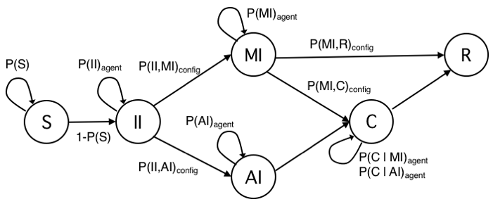
Table 1 summarizes the characteristics of model’s states.
| Symbol | Compartment | Description |
|---|---|---|
| S | Susceptible | The initial state for all individuals in the model except the ones seeding the epidemic. At each discrete time step, individuals interact through the contact network with directly connected peers and could become infected with a certain probability that depends on the number of infected peers and their infected state (II, MI, AI, or, but only for some simulations, C). |
| II | Incubating Infected | Incubating infected are Susceptible individuals that become infected. Infectivity develops in this phase, although reduced with respect to the symptomatic state, according to current medical analyses. This is the state assigned to the initial seeding nodes in simulations. Individuals stay in this state according to a probability distribution within a time frame derived from the literature. |
| MI | Mild Infected | Infected persons showing no symptoms or mild symptoms easily misdiagnosed or, due to the mildness of the condition, reluctant to self-quarantine and look for medical assistance. Persons in this state are often assumed to carry a reduced viral load with respect to those that develop full acute symptoms. MI individuals could at some point be diagnosed and contained (state C) or they remain in the same state until spontaneous recovery (state R). A special case has also been tested for the hypothesis of MI cases carrying a full viral load. |
| AI | Acute Infected | Infected persons that develop full symptoms and carry the full viral load. We assume that all AIs certainly receive a diagnose within a time frame, and then move to state C. The possibility that AI individuals are not diagnosed and thus contained exists in practice. However, in simulations, we have considered that case as not relevant for the outcome and ignored. |
| C | Contained | Infected persons that have been diagnosed and then isolated. Our base assumption is that individuals in state C do not transmit the infection to peers and move to recovery/removed (state R) according to a probability distribution within a time frame derived from the literature. The time frame is different for the case of an individual in C being previously AI or MI. The possibility of contained infected individuals spreading the disease is of course very well-known (e.g., in hospitals or other medical facilities). We have considered this case and run some simulations with different probability of transmission also from C individuals but this case is out of the scope of this work. |
| R | Recovered/Removed | This is the final state of the transition diagram reached by all individuals in our model. The transition from MI or from C depends on probability distributions within different time ranges. |
With regard to the model’s state transition diagram, we have added some context and details to the definitions given in Table 1. The assumption we made for state II is that it is infectious with a reduced viral load. Same assumption of reduced viral load has been made for state Mild Infected (MI), both at half the full viral load of state Acute Infected (AI). These are simplifying assumptions, based on medical reports (Li et al. 2020; Longini et al. 2005), to account for heterogeneous transmission probabilities between agents. In Appendix B, we describe the results of tests on a variant of the II state, meant to include a pre-infectious period in the incubating state. This incubating pre-infectious state is well-known in the epidemiological literature. To the best of our knowledge however, there is scant evidence for such a state in COVID-19 cases and scientific references useful to fit related parameters. For this reason, here we did not include this case in the main text and only produced a limited set of tests. Tests have been carried out with hypothetical settings and with the aim of confirming the well known effect of prolonging the epidemic duration, produced by a pre-infectious state.
To put these modelling choices into a broader context, it should be recalled that a state representing the disease incubation time has a long tradition in deterministic and stochastic models in epidemiology (Holme & Saramäki 2012). Among these, the standard SEIR dubbed it Exposed (Brauer 2008), which became Latent in other SLIAR models, specifically refers to incubating but not infectious persons (Arino et al. 2006;Li et al. 2020). Others, such as Gumel et al. (2004), studying the 2002-2003 SARS epidemic, did not consider a specific state for those incubating the disease not being infectious. Rather, they defined an Asymptomatic state as the first stage for all susceptible cases turned infected. In that state, persons are infectious and could possibly be quarantined or develop a fully symptomatic state. These approaches were not suitable for our goals. Regarding the current COVID-epidemic, different epidemiological studies analyzing samples from China and Singapore outbreaks reached the conclusion that individuals could develop infectivity in the incubation period (Ganyani et al. 2020;Li et al. 2020). As this possibility is relevant for our study, we have included the Incubating Infectious (II) state with the specific meaning of modelling the time period of infectivity during the disease incubation. The probability distribution of the time spent in this state has been obtained from Li et al. (2020).
The distinction between symptomatic and asymptomatic infected individuals was originally introduced by Longini et al. (2004) as an extension of the standard SEIR model. They postulated the fundamental assumption that only symptomatic cases self-isolate (e.g., home confined, hospitalized). Most recent conveniently customized epidemic models, are based on this distinction (Brauer 2008). Following the introduction of the two classes for the symptomatic and the asymptomatic cases, models have attempted to manage different social impacts. In Brauer (2008), two new classes are added to represent different forms of social distancing: Generic quarantine for the asymptomatic and specific isolation for the symptomatic. The quarantine state is useful for modelling the dynamic of the contagion when a social distancing policy is enforced by the public health authority (e.g., national/federal state, regional/local authority) in order to limit contacts between casual susceptible individuals and undiagnosed infected individuals, untested and often asymptomatic (Di Domenico et al. 2020). On the other hand, symptomatic infected are supposed to be diagnosed and strictly isolated, for example in a medical facility or hospital, within a certain time frame from the outset of symptoms or after a positive test.
With respect to our goal, we have considered the quarantine state as not strictly necessary. What is most important is to account for the ability to spread the contagion of all undiagnosed infected individuals. Thus, we do not distinguish whether the final attack rate was produced by reducing contacts (as for isolation measures such as generalized quarantine) or because of reduced infectivity; in both cases the final attack rate is the same. Consequently, in our model, we have included only two states called Mild Infected (MI) and Acute Infected (AI). Next, we added a single Contained (C) state for all individuals infected, diagnosed, and restricted. For our research goal, the Contained state serves the purpose of modelling those whose ability to spread is greatly reduced by means of personal containment measures, with respect to others without limitations (or only subject to a general social distancing policy).
With regard to the infectious states, we make the assumption that in the final phase of the epidemic wave, information networks such as the press and generic public opinion makers, will be primarily influenced by the dynamics of the Acute Infected and the Contained classes, as recorded by official statistics, with risks brought by the mostly unknown Mild Infected class not well acknowledged. The emphasis over observable AI and C states and the uncertainty regarding the mostly speculative MI state would put public health authorities under pressure for immediate li of isolation measures based on the dynamics of the former two states, and instead would assess with great difficulty the behaviour of the third one
The last state of our model is the traditional Recovered/Removed (R), which accounts for all individuals that end the epidemic process. In this work, we do not consider the case of re-infection and temporary immunization. One reason is that we explicitly focus on the last period of the first epidemic wave and the potential risks from undiagnosed infected. As such, we assume that even in cases of temporary immunization, the rate of re-infections would not be particularly relevant in that time frame. Another reason is that at present, to the best of our knowledge, the possible temporary immunization for COVID-19 patients is still a hypothesis being investigated by medical researchers.
Final Epidemic Phase and Model Initialization
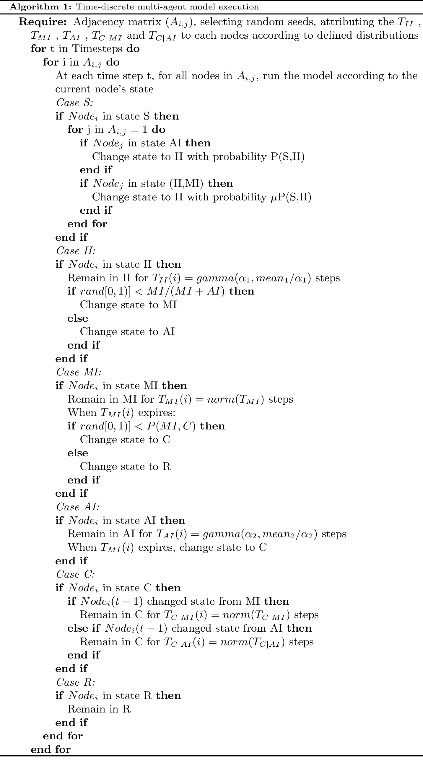
The model is run through multi-agent simulations (Bruch & Atwell 2015; Jiang & Jiang 2014) and represents contacts between agents through a static network, whose characteristics have been described in Appendix A. The basic execution of the model is described in Algorithm 1. Each iteration represents a time step in simulation time. At every time step, each node is selected in random order and, if in state S its state is checked with respect to peers, or if in other states, according to time periods specific of states II, MI, AI, and C. The probability of a node S to become infected depends on infected peers II, MI and AI, independently (\(\mu\) is the reduction factor to account for possibly reduced viral load of II and MI).
Definition of final epidemic phase
Up to this point, we have always referred to the "final epidemic phase" implicitly, with the intuitive meaning of the time period starting when public health authorities decide to lift the lockdown and other social restriction measures, and ending with the epidemic expiration. The rationale for focusing on this specific phase of an epidemic is because public health authorities should base such a critical decision on a reliable estimate of the epidemic size at that time. Only with a sufficiently precise knowledge of the epidemic size is it possible to evaluate the benefits of lifting the restrictions with respect to the risks of spreading new contagions. However, as in the case for COVID, understanding the actual epidemic size is imprecise due to many contextual factors (e.g., errors in reporting cases, different classification criteria of cases). But even more relevant than contextual factors could be the mass of infectious individuals that remain undetected and uncontained, because of the lack of generalized testing and the ambiguity of their symptoms, possibly so mild as to be misdiagnosed for a harmless condition like seasonal cold or sore throat, or absence of any visually recognizable symptom of infection (Ioannidis 2020; Kimball et al. 2020). In our model, the Mild Infectious (MI) state serves the purpose to represent those undetected cases and we focused on it as the critical factor to evaluate the risk level of the final epidemic phase. To proceed with the analysis and to compare the effects of different configurations, we introduce an operational definition of final epidemic phase as a time period measured in simulation timesteps. To specify it, we focus on the Contained (C) state, which is supposed to be known and to serve to public health authorities as the primary evidence to estimate the epidemic size. We proceeded in three steps:
- The first thing we did was to look for examples of public data of active cases of COVID-19 for the day when public authorities lifted the lockdown and to derive an approximate threshold of active cases over the population size for that day.
- We then turned to our model and assumed that the number of active cases in COVID-19 statistics logically corresponds to our C state, because both are known measurements and relate to infected cases, officially recognized and treated, at a specific time (day, timestep).
- Finally, we chose as the initial timestep of the final epidemic phase the one corresponding to a rate |C| (number of agents in C state at a given timestep) over N (population size) in our simulations equals to the threshold of active cases over the population the day a lockdown had been lifted (i.e., active cases/population size (day) \(\Rightarrow\) |C|/N (timestep)).
This simplified assumption could prove acceptable for some real cases while being unacceptable for many others, since the variety of criteria and factors that influencing government a lockdown lifting decisions is huge and difficult to describe in a single metric. However, we found that in examples used to estimate threshold active cases/population, at least the coherence between a clearly decreasing epidemic phase and the decision to lift the restrictions was always granted. In particular, we found data about active cases related to the Lombardy region in Italy (Ministero della Salute 2020), the Madrid region in Spain (Euronews 2020) and New York state (The COVID Tracking Project 2020), three cases with similar characteristics (epidemic intensity, population density, demographics). The Lombardy and the Madrid regions started lifting the lockdown on May 18, 2020; New York City started on June 13, 2020. For Lombardy and New York, we found in official statistics the number of active cases at re-opening, while for Madrid, we only found the total number of cases. However, knowing that the epidemic dynamic was similar between the Madrid region and Lombardy, we assumed the same proportion of active cases with respect to the total number of cases at re-opening. Population size was taken from official demographic statistics. The threshold given by the number of active cases over the population, calculated the day of the re-opening, was approximately included between 2.5 and 5 (x1000) cases (i.e., Lombardy (active cases/population): 27073/10M=0.0027 (May 18, 2020); Madrid region: 32.000/6.7M=0.0047 (May 20, 2020); New York state: 89995/20M=0.0045 (June 13, 2020)). For our analysis, we conventionally took the threshold of 3 (x1000) cases as a reference, and accordingly we defined the final epidemic phase as starting at the timestep corresponding to the number of agents in Contained state |C|=3, given that N=1000.
With respect to the last timestep of the final phase, ideally it would have been set when the epidemic finished. However, for practical reasons due to the presence of few outliers in the trials that lasted longer than others, which may have distorted the epidemic duration, we preferred to adopt a conventional threshold of 1 active case (x1000), as the lower limit of the final phase. The same threshold of 1 case (x1000) also appears in the literature as a reasonable threshold for considering an epidemic as under control (Brauer 2006), although it seems that a real agreement does not exist among epidemiologists about what to consider a safe proportion of active cases over the population. At any rate, it seems that the concept of final epidemic phase is worth more research in order to define better criteria for the critical decisions. However, we also recognize that it probably has to be fuzzy given that the decision of lifting social restrictions cannot be exclusively driven by scientific considerations and has to manage a trade-off between several factors. Following these considerations, we are now able to give the following definition:
Definition of epidemic size and model initialization
Our goal was to focus on the final phase of an epidemic and analyze the conditions that led to an at risk situation for public health authorities. We focused on the mostly unknown class of undetected and uncontained infectious cases (the Mild Infected state, in the model). These risky conditions arise when, from the perspective of a public health authority, known and available measures of the epidemic incidence (i.e., in our model state Contained) represent a poor estimator of the actual number of active cases. This scenario may happen when the epidemic dynamic is dominated by Mild Infected cases. Unlike the usual approach of compartmental models that start estimating a transmission probability, evaluate the theoretical reproduction number and epidemic size, then proceed downplaying them by considering the network structure and mitigation strategies, we proceeded backward. First, we estimated the hypothetical epidemic size resulting from a certain network structure (which is static, in this work, and whose details are presented in Appendix A) and possible mitigation measures (that we do not explicitly model, with the exception of one case tightly connected with our research goal), then by trial and error, we tuned the transmission probability and estimated the reproduction number. As the reference epidemic size, we made the educated guess of considering an epidemic that at expiration would have infected 30% of the total population, and the corresponding transmission probability has been calculated as equal to 0.02. The results presented in this work are all based on this working assumption. We also did tests with other epidemic sizes, namely 10% and 50% of infected at epidemic expiration. Qualitatively, they did not change the analysis and the conclusions, so in this paper we have omitted the details.
For states Incubating Infected (II) and Acute Infected (AI), we adopted a time-to-event observation model with a gamma distribution of the time \(T_{II}\) and \(T_{AI}\) an individual remains in each of those states. For states Mild Infected (MI) and Contained (C), instead, we assumed a normal distribution of time \(T_{MI}\) and \(T_C\). Parameters for gamma and normal distributions, as well as of the lengths of these periods have been derived from Li et al. (2020) (in a different study Mizumoto et al. 2020), both the probability distribution and the incubation period have received a different estimation, we took Li et al. (2020) as our reference study being based on a larger sample). Regarding trials, a trial was considered invalid, thus discarded, if it produced less than 1/5 of infected nodes with respect to the average epidemic size. In all figures, each data point was averaged over at least 150 valid trials (differences due to the variable number of invalid trials not exceed 10 trials). Five seed nodes were used in simulations, a choice that represented a good trade-off in order to reduce the number of invalid trials without relevant effects to the average number of infected nodes. Figure 2 describes the model initialization with actual transitions and probabilities.
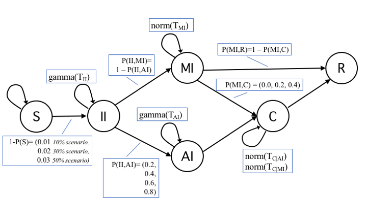
Table 2 presents a description of transition probabilities and of their values. The list of base settings for simulations is in Table 3.
| Probability | Description | Values |
|---|---|---|
| P(S) | p. to remain susceptible. It is fitted empirically according to the epidemic size at epidemic expiration that has been assumed. \(P(S) = 1- P(S,II)\). | 0.98 |
| P(S,II) | p. to get infected (transmission rate). Empirically evaluated. \(P(S,II) = 1- P(S).\) | 0.02 |
| P(II) | p. to remain in incubation state. The probability is defined as the probability distribution over the time range \(T_{II}\). | For each node \(gamma(T_{II})\), with \(T_{II}\) in [2,14], as estimated in (19), with k = 3 and mean = 8. |
| P(II,MI) | p. to move from the incubation state II to the MI state. This is the main unknown of the study. | Simulations have been run with different values for the pair AI:MI=(10:90, 20:80, 40:60, 60:40). |
| P(II,AI) | p. to move from the incubation state II to the AI state. | See P(II,MI) values. |
| P(MI) | p. to remain in state MI. The probability is defined as the probability distribution over the time range \(T_{MI}\). | For each node, \(norm(T_{MI})\), with \(T_{MI}\) in [2,7], as estimated in (19). |
| P(MI,C) | p. to move from MI to C. It measures the odds of an MI individual to be diagnosed and thus isolated. | The worst case scenario is to consider P(MI,C)=0, meaning no MI is detected and isolated. We also considered other values, i.e., 0.2 and 0.5, to account for increasing proportions of MI being detected and contained. |
| P(MI,R) | p. to recover for a MI individual. The probability depends to P(MI) and P(MI,C). | When \(T_{MI}\) steps expire, the node in MI move to R (unless previously moved to C). \(P(MI,R)=1-(P(MI)+P(MI,C))\). |
| P(AI) | p. to remain in state AI before being moving to C. The probability is defined as the probability distribution over the time range \(T_{AI}\). | For each node, \(norm(T_{AI})\), with \(T_{MI}\) in [2,7], as estimated in (19). |
| P(AI,C) | p. to move from AI state to C. It depends only on the value of P(AI). | When \(T_{AI}\) steps expire, the node in AI move to C. \(P(AI,C)=1-P(AI)\) |
| P(AI,R) | p. to recover for an MI individual without being diagnosed and contained. We assume this case as non-existent. | \(P(AI,R)=0\). |
| P(C|MI), P(C|AI) | p. to remain in C state. The evaluation of this probability is different for nodes arrived in state C from MI or from AI, being the time intervals completely distinct for the two cases. The probability then is defined as the probability distribution over two time ranges \(T_{C|MI}\) and \(T_{C|AI}\). | For each node, \(norm(T_{C|MI})\), with \(T_{C|MI}\) in [2,5] if the node was previously in state MI, or \(norm(T_{C|AI})\), with \(T_{C|AI}\) in [14,30] if the node was previously in state AI. The time ranges are defined from medical reports and (19). |
| P(C,R) | p. to recover from C. It depends on the value of P(C|MI) evaluated with respect to \(T_{C|MI}\), for agents previously in MI state. It depends on the value of P(C|AI) evaluated with respect to \(T_{C|AI}\), for agents previously in AI state. | For each node, when \(T_{C|MI}\) or \(T_{C|AI}\) steps expire, the state changes from C to R. |
| P(R) | p. to stay in R state, our final state. | \(P(R)=1.0\). |
| Parameter | Values |
|---|---|
| Population size (Network size) | 1000 |
| Seed nodes | 5 |
| Time steps | 150 |
| Epidemic size at the extinction | 30% of the population (assumption) |
| Probability of transmission (full viral load) | 0.02 (calculated from epidemic size at the extinction) |
| Reduction factor (reduced viral load) | \(\mu = 0.5\) (approximated from literature) |
| Latency time | time steps=[2,14], mean=8 (approximated from literature) |
| Infectious time - Acute Infected | time steps=[2,7], mean=3 (approximated from literature) |
| Infectious time - Mild Infected | time steps=[2,7], mean=4.5 (approximated from literature) |
| Isolation period - Acute Infected | time steps=[14,30], mean=22 (approximated from literature) |
| Isolation period - Mild Infected | time steps=[2,5], mean=3.5 (approximated from literature) |
| Proportions of Acute Infected and Mild Infected | AI:MI=(10:90, 20:80, 40:60, 60:40 ) (configurations tested) |
| Prob. of Mild Infected becoming Contained | P(MI,C)=(0.0, 0.2, 0.5) (configurations tested) |
Model Execution
The model has been executed to test various configurations and parameter settings. The results are presented here by starting from the basic epidemic dynamic, which has parameters values listed in Table 3.
Basic epidemic dynamics
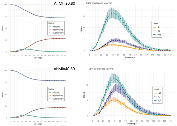
First, we ran our model to obtain the basic epidemic dynamics related to agent states. Figure 3 shows the basic state dynamics (on the left: Susceptible, Infected (as II+AI+MI+C), and Recovered; on the right: AI, MI, and C), with the additional detail of the 95% confidence intervals, with respect to the trials, of MI, AI, and C states, again for the two proportions AI:MI equals to 20:80 and 40:60. A particular aspect to note is the difference in the behaviour between Mild Infected and Contained states during the decreasing epidemic phase: for AI:MI equals to 20:80, MI dynamic dominates that of C’s, while for AI:MI equals to 40:60, the two dynamics largely overlap. This is a relevant difference that, in following sections, we will analyze through the results of several experiments aimed at testing the rate |MI| over |C| (with |x| indicating the number of agents in state x at a given timestep). We will discuss the meaning of that rate as a risk metric for the final epidemic phase.
The descriptive statistics are reported in Table 4, which is divided in three sections. Two present statistics of agents states, respectively for AI:MI proportion equals to 20:80 and to 40:60 (i.e., this means that in the first case the probability that an agent in Incubation Infected (II) state has to become Acute Infected (AI) is 0.2 and to become Mild Infected (MI) is 0.8, similarly for the second case with probability of 0.4 and 0.6 respectively). All the statistics of Table 3 are calculated on the time series produced by averaging the results of valid trials for each timestep, which in Figure 3 are represented with the dashed lines.
First, we have reported states corresponding to the classical SIR classification, with the aggregated state Infected summing up all infectious states: II (Incubating Infected), AI (Acute Infected), MI (Mild Infected) and C (Contained). Then, we reported a detailed view of all specific states, with the R (Recovered) decoupled in the two factors, the nodes recovering from AI (RAI) and those recovering from MI (RMI). It is worth note that the maximum value for Susceptible (S) nodes equals to 995 (given that 1000 is the population size), because five are the seed nodes, starting in state Incubation Infected (II).
The bottom part of Table 4 shows the results of Welch’s t-test, run to check whether the different means of the samples should be interpreted as the results of the models with the two configurations of AI:MI have different means for the number of agents.
In our case, we tested two pairs of independent samples: i) the time series of the Mild Infected (MI) state for the configuration AI:MI=20:80 and the MI time series corresponding to AI:MI=40:60; and ii) the same two configurations of AI:MI, but testing the time series of the Contained (C) state. The choice of these two states is motivated by the fact that they are key for the risk metric regarding the final epidemic phase, as we will describe in the following sections. In both cases, the Welch’s t-test does not support the validity of the null hypothesis, suggesting that the two pairs of samples have different means. The use of the Welch’s t-test, instead of the more common Student t-test, is suggested by the different variances of the samples tested, while a limitation of the results derives from the assumption of normal distribution of the Welch’s test, which is not verified in the MI and C time series, as the descriptive statistics demonstrate.
| configuration: AI:MI=20:80 | ||||||
|---|---|---|---|---|---|---|
| state | mean | sd | median | max | skewness | kurtosis |
| Susceptible | 805.80 | 98.14 | 757.47 | 995.00 | 0.77 | -0.96 |
| Infected (II+AI+MI+C) | 21.35 | 19.81 | 14.11 | 56.36 | 0.54 | -1.27 |
| Recovered (RAI+RMI) | 172.86 | 109.01 | 218.03 | 284.49 | -0.47 | -1.44 |
| II | 12.59 | 11.71 | 8.43 | 33.85 | 0.57 | -1.22 |
| MI | 6.12 | 5.82 | 3.91 | 16.55 | 0.54 | -1.26 |
| AI | 0.94 | 0.95 | 0.58 | 2.73 | 0.48 | -1.34 |
| C | 1.70 | 1.62 | 1.19 | 4.63 | 0.48 | -1.28 |
| RAI | 21.18 | 17.73 | 23.76 | 43.20 | -0.04 | -1.73 |
| RMI | 151.67 | 92.09 | 194.27 | 241.29 | -0.57 | -1.34 |
| configuration: AI:MI=40:60 | ||||||
| state | mean | sd | median | max | skewness | kurtosis |
| Susceptible | 839.04 | 73.35 | 796.94 | 995.00 | 1.04 | -0.48 |
| Infected (II+AI+MI+C) | 20.22 | 19.89 | 12.07 | 58.16 | 0.66 | -1.07 |
| Recovered (RAI+RMI) | 140.73 | 83.38 | 183.30 | 218.51 | -0.63 | -1.27 |
| II | 11.12 | 11.24 | 6.57 | 32.97 | 0.71 | -0.99 |
| MI | 4.08 | 4.21 | 2.29 | 12.23 | 0.70 | -1.01 |
| AI | 1.76 | 1.83 | 0.99 | 5.54 | 0.63 | -1.09 |
| C | 3.27 | 3.06 | 2.27 | 9.15 | 0.56 | -1.16 |
| RAI | 20.7 | 18.1 | 18.9 | 46.3 | 0.12 | -1.68 |
| RMI | 138.66 | 81.74 | 181.41 | 213.88 | -0.65 | -1.26 |
| Welch’s unequal variances t-test | ||||||
| MI data (AI:MI=20:80 and 40:60) | C data (AI:MI=20:80 and 40:60) | |||||
| t = 3.3699, df = 254.93, p-value = 0.0008685 | t = -5.3708, df = 213.06, p-value = 2.045e-07 | |||||
| 95% CI | [-2.1434043 -0.9924822] 95% CI | |||||
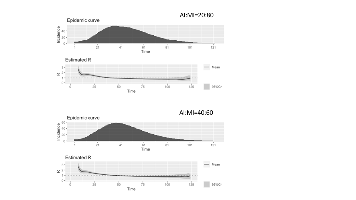
With Figure 4, we give an estimation of the reproduction number R related to our model’s epidemic dynamics. Various statistical methods have been proposed for compartmental models described through differential equations, less so for agent-based models (Dietz 1993; Driessche 2017; Jones 2007). However, Cori et al. (2013) presented a tool that produces statistically robust analytical estimates of R based on the incidence time series and quantifies temporal changes in the transmission intensity of epidemics. The tool is called EpiEstim (Estimate Time Varying Reproduction Numbers from Epidemic Curves)1 and by using it, we employed the parametric_si method by using parameters for the serial interval distribution as retrieved in Nishiura et al. (2020). In assuming the accurateness of the reproduction number when a specific network structure is considered, however, a word of caution is appropriate, because it is a complex task with many subtleties that current available software libraries, like the EpiEstem, do not typically account for. First, when simulations over networks with heterogeneous degree are performed, a correction for degree heterogeneity should be applied in R0 evaluation, as described by Olinky & Stone (2004). A second correction to R0 estimation should be applied to account for network clustering, as explained by Molina & Stone (2012). The network adopted in this work exhibits both features. However, to achieve high accurateness in R0 calculations, other network characteristics are important, such as degree (dis)assortativity and degree-clustering correlation. Again, these features are probably present in scale-free networks. The standard procedure to compute R0 numerically, for epidemic models on heterogeneous clustered networks has been presented in (Danon et al. 2012; Machens et al. 2013; Molina & Stone 2012). Therefore, summarizing this short discussion of R0 evaluation, the results produced by simplified algorithms that, not taking into account all important network features, do not apply corresponding corrections and procedures, should be regarded as broad approximations of the actual epidemic reproduction number, possibly useful to show the general trend of the epidemic, but not as accurate as required to assess the epidemic dynamic for prediction purposes.
In Figure 4, we present the results for the two AI:MI configurations 20:80 and 40:60. The incidence is the number of infected agents at each timestep, calculated as the sum of infectious states (i.e., II, AI, MI, and C). Comparing the two estimates, it could be observed that the series for AI:MI=40:60 starts from higher values than the series for AI:MI=20:80 due to the higher incidence (a larger proportion of Acute Infected agents produces a higher incidence due to the assumption of reduced viral load of Mild Infected agents). However, values of Rt smaller than 1 decreases faster, due to the larger number of Contained agents that reduces the spreading of the contagion.
Epidemic dynamics and final phase
After the presentation of our model’s basic descriptive statistics and behaviour, we analyze in more details the effects, on the final epidemic phase, of different configurations and parameter fitting. In particular, we start with considering how the different, hypothetical, proportions of Acute Infected (AI) agents and Mild Infected (MI) change the epidemic dynamic, including its duration, measured with respect to the final phase. Table 5 presents, for four configurations of AI:MI, the values of the peaks of the three main states (i.e., AI, MI, and C), and information about the corresponding final phases. Figure 5 gives a visual representation of the same data. Together these results confirm what we already commented before, that above a certain proportion of AI:MI, with the number of Mild Infected (MI) exceeding the Acute Infected (AI), the epidemic dynamic becomes clearly dominated by the MI class, which represents the unrecognized, uncertain mass of infected individuals. In our simulations, configurations with AI:MI equals 10:90 and 20:80 represent this case, while the dominance disappears and ultimately reverses with AI:MI equals 40:60 and 60:40. This is an unsurprising system behaviour, but we believe it is worth highlighting for its potential consequences on the ability of forecasters and public health authorities to predict the epidemic evolution and safely manage the risk of the re-opening. What our model shows is that if one infectious class could become dominant and if this class mostly escapes from official measurement (e.g., asymptomatic, misdiagnosed, untested because of insufficient testing efforts, unwilling to be tested, and so forth), then it is possible that the overall epidemic dynamic results out of control when social restriction measures are lifted. In this context, "out of control" should be interpreted restrictively, meaning that the overall system dynamic is dominated by a factor that is unknown to controllers and that operating on those factors directly accessible to controllers does not permit to obtain a proportional effect on the unknown ones. We do not make any inference about practical consequences, like the odds of new outbreaks or the increased pressure on medical facilities. In addition, it should be stressed that ours is a mechanistic model aiming at describing system properties, not to be misinterpreted as a forecasting model. This comment to clarify that the apparent threshold of AI:MI equals 40:60 for a largely overlapping dynamics between Acute Infected (AI) and Mild Infected (MI) has a meaning only relative to our model and settings, it should not be taken as an indication of a threshold for real cases. In real epidemic scenarios, a threshold above which the class of undetected cases becomes the dominant factor of the epidemic is, to the best of our knowledge, still unknown for COVID-19 as well as for other epidemics that could present the problem of a large proportion of undetected cases. To conclude this discussion, in our work, an epidemic is said to be out of control if public health authorities evaluate the progression with respect to official statistics (the Contained (C) class and part of the Recovered (R)), but the knowledge of those classes does not provide a reliable estimate of the larger and dominant class of undetected infectious MI.
Other observations could be made about the final epidemic phase resulting from the different configurations. Again from Table 5 and visually from Figure 5, it emerges a relationship between the AI:MI proportion and the perceived duration of the whole epidemic and of the final phase. Clearly, here we did not considered the case of re-infection or epidemic relapse, which will be the subject of a future work, and our aim is limited to analyze the possibility to have unmanaged risks. Considering risks, it is paramount to focus on the perception of risk by decision makers. In our cases, the beginning of the final phase represents a milestone in risk perception, because it signals the passage from a phase of pure containment of the havoc caused by the epidemic, to a phase where the benefits of removing limitations are weighted against the perceived residual risks. The end of the final phase is the second milestone of risk perception, because it signals the end of the danger and the return to normal conditions. Our simulations should make more evident a second unsurprising, but again worth to be highlighted, effect of the dominance by the class of undetected MI cases: the risk perception based on observable cases could be dangerously misleading with respect to the reality of an epidemic dynamic. The most evident example reflecting this mismatch between perceived and real risk could be observed in the consequences of insufficient testing for COVID-19 that plagued most countries so far. Thornton (2020) reported how "lack of tests and inadequate testing was not helping the authorities prepare for the crisis or give its people the right message about the need for caution and social distancing", an op-ed in Nature (“The COVID-19 testing debacle” 2020) commented that "as economies reopen, insufficient testing relinquishes control of COVID-19 because new virus clusters elude detection and spark new outbreaks", while Italy had to introduce mandatory COVID-19 testing for tourists returning from summer holidays after a surge of cases, mostly due to the common wrong belief, produced by previous lack of testing, that young people were at low risk of infection (Stefanello 2020). All these cases, and the countless others of the same kind, are mostly due to the fact that the class of mild infectious individuals is largely underestimated and unknown in its characteristics. As consequence, risk is evaluated mostly based on the only class of individuals known at the time of reopening, which is of those that have been recognized as infected and then subject of containment measures. Our main contribution is then of a model and some simulation results representing mitigation strategies based on identification and containment of mild infectious cases, an activity that has been now wildly recognized as necessary, but still relatively untested and not fully analyzed. To this end, we will introduce a simple metric based on the rate between mild infectious (MI) and contained (C) cases in the final phase, to assess the alignment between the perceived and actual risks.
Our simulations suggest that the larger the dominance of the Mild Infected (MI) class is (see panels AI:MI equals 10:90 and 20:80 in Figure 5), the earlier the final phase starts and, while less than proportionally, also the earlier it ends. This produces a large misalignment between the risk perceived (approximated through the Contained agents, representing known active cases) and the actual risk (given by the actual size of the Mild Infected). The misalignment between perceived and actual risk is absent for cases without the dominant MI (see panels AI:MI equals 40:60 and 60:40 in Figure 5). In the following section, we propose a quantification of the misalignment between perceived and actual risk by means of a simple metric and introduce the possible dependence from other factors.
| AI:MI | AI peak timestep (cases) \(\pm\)CI95% | MI peak | C peak | Final Phase start timestep | Final Phase end | Final Phase duration No. timesteps |
|---|---|---|---|---|---|---|
| 10:90 | 41 (1.71±0.26) | 36 (21.±2.91) | 47 (2.93±0.25) | 48 | 77 | 29 |
| 20:80 | 37±3.19 (2.73±0.45) | 38±3.02 (16.55±2.21) | 45±3.16 (4.63±0.38) | 67 | 93 | 26 |
| 40:60 | 38±2.63 (5.54±0.71) | 40±2.64 (12.23±1.46) | 43±2.88 (9.15±1.18) | 83 | 106 | 23 |
| 60:40 | 47 (7.14±1.27) | 48 (7.40±0.88) | 59 (13.58±1.74) | 105 | 121 | 16 |
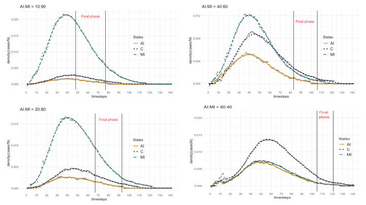
For each panel, the proportion AI:MI is reported, and the final epidemic phase is indicated, corresponding to values of |C|=3 and |C|=1 in the descending part of the epidemic dynamic.
Effects of containment of Mild Infected (MI) in the final epidemic phase
In this subsection, we introduce the variant representing the outcome of possible epidemic mitigation strategies. We assumed that a fraction of the Mild Infected (MI) cases is detected and thus moves to the Contained (C) state, rather than remaining in the MI state until the final transition to the Recovered (R) class. With respect to the model, this means setting the probability P(MI,C) greater than zero (i.e., values 0.2 and 0.5 have been tested), which means that at each timestep, each agent in the MI state could move to C with that probability. With respect to real cases, we may think to this variant as the result of increased testing efforts and screening campaigns. On the other hand, with respect to the system dynamics, the direct effect should be to reduce the epidemic incidence due to the time spent by former MI cases as contained, thus not spreading any longer the contagion (with a consequential reduction of the reproduction number Rt). But of particular interest for our analysis, there is also a secondary effect on the rate between the number |MI| of undetected infectious and the number |C| of contained cases at each timestep, because as mentioned, this represents a critical rate in the final epidemic phase for evaluating the risk caused by a possible dominant class of undetected infectious MI.
In simulations, we tested for each of the two proportions AI:MI equals to 20:80 and to 40:60, two values of the probability P(MI,C), equals to 0.2 and to 0.5. The two proportions AI:MI have been selected because, as seen before, they produce two clearly different system dynamics, one dominated by the class MI, the other with a substantial overlap between the MI and the C curves. The goal is to compare the effects of the two cases with P(MI,C)>0 the case of P(MI,C)=0. In particular, we measured the different peaks of MI and C curves, and changes in the corresponding final phases. Table 6 compares the results between the different configurations. The effects of the probability of Mild Infected agents to move to Contained state are observable in the peak variations, with the MI peak that tends to decrease and the peak of C that tends to increase. The effect on the peak of the dynamics is not proportional to the probability of removal of MI agents, as expected from the non-linear relationship between the dynamics. Interesting is the temporal effect. Final phases tend to start later and to last longer by increasing the P(MI,C), thus reducing the number of Mild Infected (MI). The same relationship between beginning of the final phase and its duration was already observed for the different configurations with P(MI,C)=0 of Figure 5: the larger the proportion of MI agents, the earlier the final phase begins, and the longer is the duration.
A comment on these results is that it should be considered that epidemic classes (e.g., undetected infectious MI and contained cases C) are co-evolving when a mitigation strategy like increasing testing frequency is put in place. Therefore, on the one hand, we should expect a net effect of reducing the incidence of the epidemic, because a number of previously uncontrolled infectious cases (the Mild Infected (MI) in our model), free to spread the contagion, becomes subject to restrictions and isolated (our class Contained (C)). The reproduction number Rt would decrease, too. However, the epidemic would not necessarily have a shorter duration. In summary, while it could be stated that mitigating efforts aimed at reducing the number of undetected asymptomatic or mildly symptomatic cases are beneficial for reducing the epidemic incidence and the reproduction number, it should also be observed that the problem of evaluating the expected benefit of a certain detection effort (e.g., a testing campaign having the goal of detecting 30% of undetected infectious cases in a population) is of difficult resolution. First, there is the uncertainty regarding the real size of the undetected infectious population (our AI:MI proportions) that could change considerably the results and the costs for the mitigation strategy. Then, there is the non-linear relationship between the extent of a mitigation effort (our probability P(MI,C)) and its outcome. As a consequence, it would be difficult to produce a reliable cost/benefit analysis between mitigation efforts with different target goals (e.g., in our case between mitigation campaigns having different P(MI,C)).
| configuration: AI:MI=20:80 | |||||
|---|---|---|---|---|---|
| P(MI,C) | MI peak timestep (cases) \(\pm\)CI95% | C peak | Final Phase start timestep | Final Phase end | Final Phase duration No. timesteps |
| 0.0 | 38±3.02 (16.55±2.21) | 39±3.16 (4.63±0.38) | 67 | 93 | 26 |
| 0.2 | 39±3.03 (14.48±1.61) | 46±2.84 (8.90±1.22) | 69 | 94 | 25 |
| 0.5 | 46±3.92 (10.23±1.91) | 50±4.15 (12.36±2.26) | 86 | 105 | 29 |
| configuration: AI:MI=40:60 | |||||
| P(MI,C) | MI peak timestep (cases) \(\pm\)CI95% | C peak | Final Phase start timestep | Final Phase end | Final Phase duration No. timesteps |
| 0.0 | 41±2.64 (12.23±1.46) | 47±2.88 (9.15±1.18) | 83 | 106 | 23 |
| 0.2 | 36±3.09 (11.16±1.59) | 38±3.23 (13.20±2.41) | 76 | 102 | 24 |
| 0.5 | 51±4.09 (10.48±2.23) | 50±4.32 (17.28±3.43) | 92 | 119 | 27 |
Effects of different durations of Mild Infected (MI) and Contained (C) States
In this last part of the section dedicated to the main experimental results, we focused on two critical parameters:
- The average duration of the Mild Infected (MI) state (TMI).
- The average total duration of the Acute Infectious (AI) and the Contained (C) state (TC).
The rationale to focus on these two factors is because their combined effect could influence, to a remarkable extent, the level of risk associated to the final epidemic phase. Conversely, the sensitivity of the level of risk with respect to these two factors seems often overlooked in epidemiological literature, where it never occurred to analyze the combined effect of the two. In addition, there are solid reasons to consider these two parameters as still largely uncertain, which make them particularly relevant for our analysis. On the one hand, several clinical COVID-19 studies have presented estimates on samples of asymptomatic cases regarding the duration of their condition (Park et al. 2020; Yan et al. 2020), but they are still early results on few cases and, in addition, empirical evidences presenting seemingly abnormal durations have been reported (Li et al. 2020; Tan et al. 2020). In general, it looks like a solid understanding of the duration and temporal distribution of the asymptomatic and mild infectious state is still lacking. On the other hand, uncertainty affects the average duration of the time period from the onset of full symptoms to the final recovery/removal too. This time period is composed by the period an individual with full symptoms remains untested and uncontained (i.e., Acute Infected (AI), in our model), and the period under containment measures (i.e., our Contained (C) state). With respect to the onset of full symptoms, official data record the day an individual has been tested positive and thus recognized as a patient in need of containment, whereas for the time it took from the onset of full symptoms to the testing, the evidences are sketched and official statistics are heavily influenced by the actual organization and efficiency of testing procedures, availability or shortage of testing equipment, possible clogging of hospital facilities, and behavioural responses of individuals at the onset of symptoms (“The COVID-19 testing debacle” 2020). With respect to the period in containment state, official statistics in this case are reliable (e.g., hospitalization duration, mandatory at-home quarantine duration), but evidences have been often reported about cases with anomalous long persistence of the infection (D’Ardes et al. 2020). Overall, to us it seemed worth to investigate more closely what the combined effect of different values of these two factors could be, both considering the contingent situation of COVID-19 and in general, as a system-level analysis of epidemic dynamics.
To ease understanding, Table 7 serves as a reminder showing the parameters and state transitions considered in the tests, together with settings tested for parameters TMI and TC. Values of mean time periods for the two parameters are: (3, 5, 7, 9) timesteps for mean TMI, and (10, 14, 18, 22, 26) timesteps for mean TC. The choice of values wish to reflect the degree of uncertainty surrounding the evaluation of these two time periods. For TMI, the usual average duration of a common flu (e.g. 5-7 days) is often used as a reference, but both shorter and larger durations have been proposed as better estimators of COVID-19 asymptomatic cases (Kimball et al. 2020). With regard to TC, official statistics usually vary between 14 and 21 days for hospitalized patients (Centers for Disease Control and Prevention 2020; World Health Organization 2020), while the typical mandatory at-home quarantine period is 14 days. Also for this factor, shorter and longer mean time periods have been discussed (D’Ardes et al. 2020).
| Diagram | Probability | Tests |
|---|---|---|
 |
P(MI): p. to remain in state MI. The probability is defined as the probability distribution over the time range TMI. |
Values (timestep): TMI, mean=(3,5,7,9) TC, m ean=(10,14,18,22,26) Tests: TC x TMI |
| P(C): p. to remain in C state. The probability then is defined as the probability distribution over the time ranges TC. | Metric: |MI|/|C| =
|
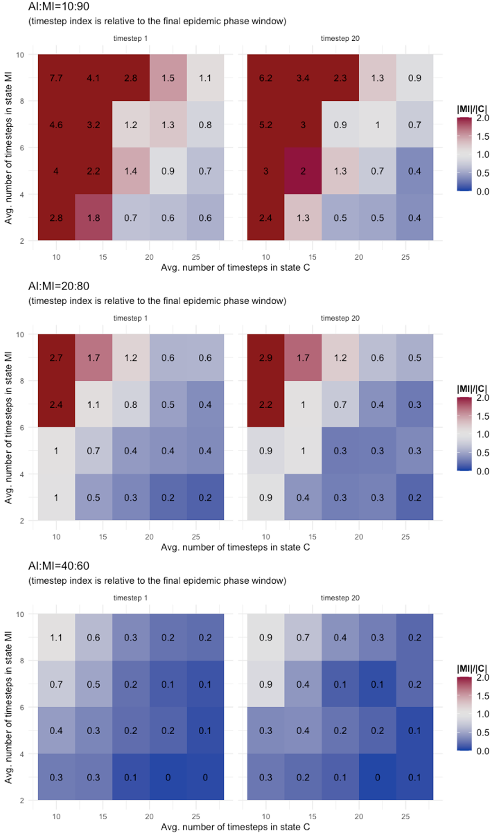
Results of tests are reported as annotated heatmaps in Figure 6. The metric used is the rate between the number of cases in state MI and those in state C (i.e., |MI|/|C|) at two timesteps: the first timestep of the final epidemic phase (indicated as timestep 1) and the 20th timestep of the final phase (indicated as timestep 20). The choice of the 20th timestep is conventional, as one of the last final phase timestep in all the tested configurations. The color scheme adopted should give a clear visual indication of changes in the risk metric:
- Red gradient for values of \(|MI|/|C|\gg1\) meaning that MI dominates C, thus the risks brought by the MI are possibly out of control;
- White gradient for values of \(|MI|/|C|\approx1\) meaning that C and MI classes have similar dynamics, thus the observable C class could serve as a good proxy to manage risks from MI;
- Blue gradient for values of \(|MI|/|C|\ll1\) meaning that class C is the dominating dynamic, thus no systemic risks are introduced by the MI class.
As it clearly results from Figure 6, the presence of a threshold at AI:MI=40:60 is confirmed by these tests too: For AI:MI=40:60 the potential risk brought by the Mild Infected (MI) cases is low and limited to few combinations of parameter values, (TMI, TC)=(9,10; 7,10), representing the extreme scenario of long permanence in asymptomatic state and short containment period for symptomatic cases. Different is for AI:MI=20:80 and 10:90. For these configurations and for both parameters, the risk metric crosses all three levels (red, white, and blue) and for values not only associated to extreme scenarios. A conclusion that could be draw from these results is that for large rates of undetected mild infectious cases, it is the combination of the two parameters TMI and TC to determine the level of risk. Therefore, it does not suffice to have good accuracy on the evaluation of just one of the two, it is needed on both, because underneath there is a co-evolving system dynamic. Other comments are that the severity of risk exposure might grow more than proportionally by increasing the fraction of undetected infectious, and that, conversely, there is no evidence of a sensible reduction in risk exposure during the final epidemic phase.
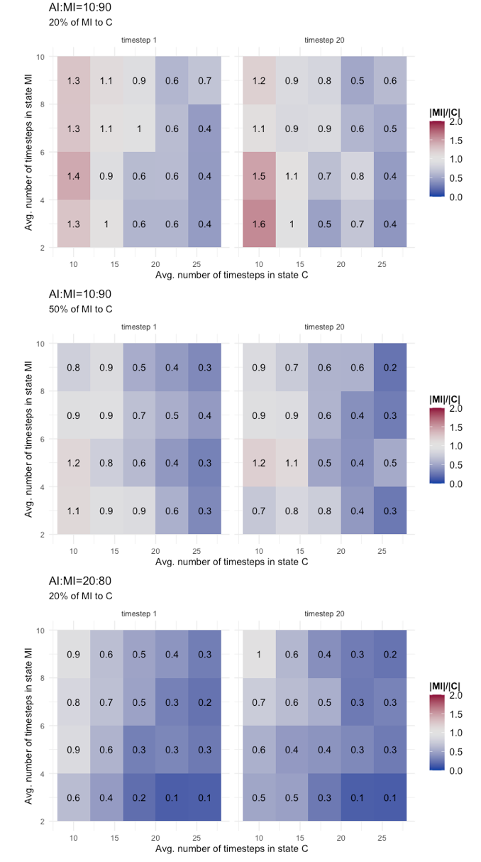
As the final result that we present, we made an additional step and replicated the same tests discussed with the heatmaps of Figure 6, but this time considering that MI agents could be detected and contained with a certain probability (i.e., P(MI,C)=(0.2, 0.5)). We have already studied the effects of this variant on the basic epidemic dynamics, here we want to see the effect on the risk metric. Table 8 shows the results. They are separated for AI:MI=10:90 and 20:80, and compare mean and standard deviation of |MI|/|C| values at timestep 1 and timestep 20 of final phase for configurations with P(MI,C) equals 0.0, 0.2, and 0.5. As expected, the result is that there is an improvement (i.e., a reduction of mean value and standard deviation) when P(MI,C) is greater than zero, shifting the risk profile towards a low risk scenario, as also showed with more details in the heatmap of Figure 7. We run a Tukey HSD test, which compares at 95% confidence interval the difference in means and adjusted p value of two independent time series, to evaluate if improvements provided by the configurations with P(MI,C)>0 significantly change the mean of the distribution. The indication provided by the Tukey test is contrasted. For AI:MI=10:90, both the difference between configuration with P(MI,C)=0 and P(MI,C)=(0.2,0.5) turned out to be significantly different, but not so the difference between P(MI,C)=0.2 and P(MI,C)=0.5. For AI:MI=20:80, instead, the difference between P(MI,C)=0.0 and P(MI,C)=0.2 is not significantly different (we did not reported the results with P(MI,C)=0.5 because in that case all values of |MI|/|C| become less than one, meaning a low risk scenario). These results seem to suggest that in a scenario strongly dominated by one epidemic class (AI:MI=10:90 in our case), testing efforts aimed at reducing the prevalence of the dominant class could be very effective, although it is difficult to calibrate them because the gains are not linear, so it is possible that considerably increasing the efforts produce a less-than-expected gain (i.e., as for the non significantly different mean of P(MI,C)=0.2 and P(MI,C)=0.5 series). On the the other hand, in a slightly different scenario, with a less strongly dominant class (the AI:MI=20:80 in our case), the effectiveness of a limited testing effort could be poor, because the re-balancing effect between the undetected infectious cases and the contained could be non enough to make a difference (i.e., the non significantly different mean of P(MI,C)=0.0 and P(MI,C)=0.2 series). To summarize, the scenario seems to put public health authorities in a complex situation, facing difficult choices: Depending on how large the mostly unknown class of undetected infectious individuals is, a certain testing effort could be effective but increasing it not worth the gain, or it could be largely ineffective and an increase is needed to obtain tangible results.
| configuration: AI:MI=10:90 - |MI|/|C| basic statistics | ||||
|---|---|---|---|---|
| Control | Timestep relative to Final Phase | Mean | SD | |
| P(MI,C)=0 | t_1 | 2.19 | 1.81 | |
| t_20 | 1.81 | 1.59 | ||
| P(MI,C)=0.2 | t_1 | 0.846 | 0.321 | |
| t_20 | 0.825 | 0.328 | ||
| P(MI,C)=0.5 | t_1 | 0.680 | 0.266 | |
| t_20 | 0.639 | 0.279 | ||
| Tukey test | Diff | Lower | Upper | p Adjusted |
| P(MI,C)=0.5 - P(MI,C)=0.2 | 0.45032 | 0.07939718 | 0.8212428 | 0.0129606* |
| P(MI,C)=0 - P(MI,C)=0.2 | -0.47714 | -0.84806282 | -0.1062172 | 0.0078252** |
| P(MI,C)=0 - P(MI,C)=0.5 | -0.92746 | -1.29838282 | -0.5565372 | 0.0000001*** |
| configuration: AI:MI=20:80 - |MI|/|C| basic statistics | ||||
| Control | Timestep relative to Final Phase | Mean | SD | |
| P(MI,C)=0 | t_1 | 0.840 | 0.692 | |
| t_20 | 0.823 | 0.713 | ||
| P(MI,C)=0.2 | t_1 | 0.458 | 0.241 | |
| t_20 | 0.424 | 0.211 | ||
| Tukey test | Diff | Lower | Upper | p Adjusted |
| P(MI,C)=0 - P(MI,C)=0.2 | -0.90705 | -1.616868 | -0.1972316 | 0.0129342* |
Discussion
In this work, we have considered several uncertain factors that play an important role in evaluating the risk of the re-opening decision. The first is that there is apparently no agreement on the appropriate time for moving from a initial phase of pure containment of the damage, to a phase when it is the trade-off between preventing the infections and restoring social activities the most challenging issue. The evidence from COVID-19 experience is that re-opening decisions depend on many contingent factors, that case-by-case may assume more or less relevance. Epidemiological and medical considerations, economic context, cultural and political motivations, and demography are all playing an important role. Moreover, considering a pandemic, not an isolated outbreak, interdependencies between regions and states are also important, so that a re-opening decision could also be influenced by the relative time a certain region/state has experienced the contagion with respect to others. Despite this heterogeneity, for all there is a time when the decision to lift the restrictions is considered and we have defined it final epidemic phase, giving a simple empirical definition that, with the many limitations that it has, was needed to define a metric of risk and confronting scenarios. In future COVID-19 studies, it would be perhaps interesting to develop a detailed analysis of re-opening time of a large set of regions/states and of the epidemiological and social conditions, as well as of the knowledge of epidemic dynamics, that were present at that time. Those studies will possibly shed a light on which factors played a major role in the decisions, what was known through official statistics, at the time, to public health authorities, and which aspects of the epidemic were instead unknown or poorly evaluated, how the decision was implemented, for example if many small adjustments were decided based on frequent observations and so forth. Comparing different situations and based on models describing the dynamics and the relations in a more abstract form, it will be perhaps possible to obtain a better picture of the overall dynamics of the pandemic, not only in terms of epidemic characteristics, but also in terms of behavioural responses and decisions taken by local authorities mutually influencing and co-evolving with the epidemic diffusion.
Next, we considered more specifically the main factor of this work: the proportion between known infectious cases and those unknown, namely the Acute Infected (AI) agents, plus the Contained (C) agents, and the Mild Infected (MI) ones, in our model. We focus on cases with a majority of MI, because that is a critical situation and represents one of the main unknown aspects of the COVID-19 pandemic. Again, our approach is not aimed at producing an epidemiological analysis, but mostly focused on a system-level analysis. Indeed, our main point in considering different proportions of AI and MI agents is that it gives, indirectly, a measure of the uncertainty of the situation. The larger the fraction of undetected MI cases, the more uncertainty is affecting the decision of public health authorities. We compared different scenarios, and found that the dynamics that we observed change completely between configurations where the MI class is clearly dominating the AI, and cases with similar dynamics. Those results, while devoid of any predictive value for real contexts, should be read as a warning to decision makers. Countless discussions have been made regarding COVID-19 asymptomatic cases and to what extent they have driven the diffusion of the contagion. Remarkable efforts have been devoted to ascertain the actual viral load and the infectivity of the incubating phase. Apparently, not equal attention has been dedicated by modelers to evaluate the effects of uncertainty, for example the effects on re-opening decisions of the error in estimating the number or the infectivity of undetected cases. This sort of system-level, risk-oriented way of reasoning did not enter in the mainstream COVID-19 discussion, so far (Ioannidis 2020; “The COVID-19 testing debacle” 2020). Tightly connected with these observations are our experiments with an increasing proportion of Mild Infected (MI) agents that become Contained (C). Stripped to its most simplified form, it represents the effects of a possible containment strategy implemented by public health authorities. In our schematic model, direct effects are straightforward (i.e., MI agents decrease and C agents increase), in reality it will not be such simple, of course. However, some results that we have presented show that one critical issue might regard the effectiveness of such mitigating strategies. As we have experienced with COVID-19, testing initiatives addressed to a large portion of the population are extremely difficult to realize, because of their economic costs, organizational burden, and possible shortage of testing equipment. Therefore, the question is not whether or not testing, but what fraction of the population of asymptomatic individuals gives the better trade-off between costs and benefits. What our work is suggesting is that answering to this question is difficult and depends on different factors. First, the effectiveness of a testing campaign may depend on the actual proportion of unknown infectious cases, whose evaluation is ridden with difficulties, as we discussed.
However, this is not enough, because there could be other factors playing an important role in making a testing campaign more or less effective and economically sustainable. We have considered two parameters, which in current COVID-19 studies have received evaluations in a relatively large range of values. They are time-dependent parameters, representing the average duration of the asymptomatic infectious phase and the average duration of the full symptomatic and officially contained phase. Again, it is a trade-off between several dimensions of uncertainty, this time regarding the number of cases and the duration of infectious states. We have showed that both the time-dependent parameters are able to strongly modify the risk level. This adds another layer of complexity, because it shows how, at system-level, the co-evolutionary dynamic of different infectious states is rich.
Conclusions
We have focused on the critical decision of lifting social restrictions, that public health authorities face to at the beginning of what we have called final epidemic phase. Our interest was mostly related to the possibility to measure and manage the risk associated to such decision. More specifically, we aimed at considering the factors possibly affected by large uncertainty at the time of the decision and influencing the risk evaluation and management in a sensible way. To this end, the current COVID-19 pandemic provides plenty of evidences of uncertainty affecting the epidemic dynamics, its defining factors, and the decision process regarding social restrictions, their enforcement and lifting.
Therefore, the study of an epidemic with severe social implications, like the case of COVID-19, is a multifaceted and interdisciplinary research goal that goes behind the typical epidemiological analyses and models, especially, in our opinion, when the focus is on the dynamics following the initial exponential growth (or past the incidence peak). Therefore, while there is certainly the need of even more accurate and precise predictive epidemiological models, for planning the emergency measures and anticipating, as much as possible, critical situations, like the shortage of required resources, other approaches are also useful. This is the case of descriptive models, aiming at producing a better knowledge of the dynamics of co-evolving processes, epidemic and behavioural, possible emergent behaviours of complex systems, and potential outcomes in different scenarios. Risk-based approaches are typical in contexts where decisions have to be taken under uncertainty.
We hope this work could be useful in particular, for suggesting future studies on epidemics aimed at complementing the traditional epidemiological approaches and predictive models. Behavioural, risk-based, economic, and sociological analyses, as well as focused studies on opinions and media, traditional and social, in the event of a pandemic like the COVID-19, are needed for a better comprehension of the mechanisms and dynamics of such a complex phenomenon. On the other hand, we also hope that our work could inspire works that openly recognize the unknown and uncertain factors of a pandemic, and the need to explicitly account for them in models and in public discussions. Evidence that is emerged from the COVID-19 experience is the unpreparedness in dealing with uncertainty in modelling and in public discourses. This is not surprising and is largely justifiable, but it has also caused problems of distorted public expectations, difficult organization, and in decision making.
Notes
- https://cran.r-project.org/web/packages/EpiEstim/EpiEstim.pdf.
- https://networkx.github.io/documentation/networkx-1.10/reference/generated/networkx.generators.random_graphs.powerlaw_cluster_graph.html.
Model Documentation
The code of the multi-agent model and simulation configurations are available on CoMSES Network - Computational Model Library as: Final Phase Epidemic Risk Model (version 1.0.0), https://www.comses.net/codebases/7a89e85b-7355-47b9-b8f5-b9b94a4a178c/releases/1.0.0/.
Acknowledgements
We would like to thank the anonymous referees for their useful contribution to this paper with their extremely detailed, competent and constructive observations.Appendix
A: Network characteristics
The network used for experiments has N=1000 and scale-free characteristics. It is an abstract network generated through the powerlaw_cluster_graph function of NetworkX package2, which is based on Holme and Kim algorithm for graphs with powerlaw degree distribution (Holme & Kim 2002).
With respect to the network choice, it should be highlighted that choosing an abstract network model represents an assumption aimed at simplifying the analysis of epidemic dynamics, at best matching only some general features of real networks. Different network configurations (e.g., differing for skewness, clustering, community structure, etc.) might considerably change the epidemic dynamics, therefore there is no general network structure really representative of real cases, which should be considered individually for an accurate analysis. Studying empirical networks or the effect of different configurations of artificial networks on the final phase and the epidemic dynamics is an interesting research subject and possibly the goal of future works.
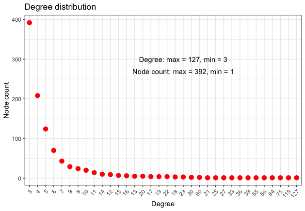
The following Table 9 presents some network metrics, while Figure 8 gives a more detailed information regarding the node degree distribution.
| Degree | Betweenness | Eigenvector | Clustering Coeff. | ||||
|---|---|---|---|---|---|---|---|
| Min. | 3.000 | Min. | 0.00 | Min. | 0.002431 | Min. | 0.0000 |
| 1st Qu. | 3.000 | 1st Qu. | 0.00 | 1st Qu. | 0.013399 | 1st Qu. | 0.1667 |
| Median | 4.000 | Median | 12.04 | Median | 0.025859 | Median | 0.3333 |
| Mean | 5.982 | Mean | 56.15 | Mean | 0.043427 | Mean | 0.3380 |
| 3rd Qu. | 6.000 | 3rd Qu. | 50.18 | 3rd Qu. | 0.061411 | 3rd Qu. | 0.4000 |
| Max. | 127.000 | Max. | 1461.16 | Max. | 1.000000 | Max. | 1.0000 |
B: Pre-infectious incubation testing
Here, we describe the results of tests on a variant of the II state definition, meant to include a pre-infectious period in the incubating state. This incubating pre-infectious state is typically indicated as the Exposed compartment in classical SEIR compartmental models (Li & Muldowney 1995) and usually refers to the initial latent phase of a contagion, before an individual develops infectivity. To the best of our knowledge, still few evidences emerged about a possibly latent state in COVID-19 cases (Lauer et al. 2020; Linton et al. 2020). The still limited number of scientific references useful for modelling that case and fitting related parameters is the main reason for our choice of not including this case in the main text. Nevertheless, we recognize the potential relevance of the case and when more epidemiological results will be available, that would be a state to model more precisely also in exploratory analyses like ours. For this work, we have limited the analysis to test some hypothetical settings, to produce an initial evaluation of possible effects of a pre-infectious period, like the known effect of prolonging the epidemic duration.
For our tests, we did not modify the transition diagram by introducing an Exposed state, but modified the mechanisms associated to the Incubating Infectious (II) state. In the original version, we assumed that the whole period, calculated for each agent from a gamma probability distribution, is infectious. In this special case, instead, we defined a fixed number of timesteps (five) at the end of the II period as infectious, while the initial timesteps, variable according to the gamma probability distribution, were not infectious. The choice of five infectious timesteps find some confirmation in Li et al. (2020), but in the light of the scant evidence retrieved so far for COVID-19 cases, it should be considered purely as an educated guess. Similarly for the incubation periods tested: The interval between 2 and 10 days has been estimated by the World Health Organization (WHO), while between 2 and 14 days is the estimate of the United States’ CDC (Worldometers 2020). Table 10 presents the results of epidemic dynamics with selected configurations (except for the II state, we used the same settings of basic epidemics dynamics with AI:MI=20:80, presented in Table 5). The results present an obvious reduction of incident cases, due to the reduced number of infectious timesteps. With respect to the epidemic duration, it is generally confirmed the expected prolongation by a clear increase of the final phase terminating timestep (column ‘Final Phase end’ in Table 5). It is particularly evident for Configurations C1 and C2, with C1 having the same settings of TII used in the original version and C2 having a reduced length of the II state duration. Configuration C3 and C4 tested different means, and still the longer duration is confirmed. With configuration C5 and C6, instead, we tried with a transmission probability much higher (0.2 instead of 0.02) and although the incidence values change considerably, the higher transmission probability seems not to have a particular effect on the duration. As said, these should be considered as very initial experiments, waiting for more solid evidence from epidemiological studies.
| Cfg | Param | MI peak timestep (density) | C peak | \(\Delta\)MI, \(\Delta\)C | Final Phase start, \(\Delta\)start timestep, \(\Delta\)time. | Final Phase end, \(\Delta\)end timestep, \(\Delta\)time. | Final Phase durat, \(\Delta\)d. No. timesteps |
|---|---|---|---|---|---|---|---|
| C1 | 1-P(S)= 0.02; mean=5 | 47 (4.24) | 52 (13.31) | +13, +14 | 109 (+42) | 130 (+37) | 21 (-5) |
| C2 | 1-P(S)= 0.02; mean=5 | 46 (4.89) | 54 (13.32) | +12, +16 | 104 (+37) | 129 (+36) | 25 (-1) |
| C3 | 1-P(S)= 0.02TII=[2,14]; mean=3 | 31 (3.04) | 42 (7.96) | -3, +4 | 77 (+10) | 92 (-1) | 15 (-9) |
| C4 | 1-P(S)= 0.02TII=[2,14]; mean=8 | 72 (2.71) | 79 (7.00) | +38, +41 | 115 (+48) | 130 (+37) | 15 (-9) |
| C5 | 1-P(S)= 0.2TII=[2,14]; mean=5 | 32 (132.23) | 44 (301.96) | -2, +6 | 79 (+12) | 84 (-9) | 5 (-21) |
| C6 | 1-P(S)= 0.2TII=[2,14]; mean=8 | 43 (102.92) | 54 (262.99) | +9, 14 | 96 (+29) | 103 (+10) | 7 (+19) |
C: No viral load reduction for incubating and mild infected
In this second special case, we considered the hypothesis that there is no reduction of the viral load for Incubating (II) and Mild Infected (MI) cases with respect to individuals developing full symptoms (AI), as suggested by some epidemiological studies, such as Zou et al. (2020). This represents another important parameter for modelling the epidemic dynamics. Here, we present a simple evaluation of the different outcomes by confronting in the two cases (reduction factor \(\mu\)=1.0 or =0.5) the basic epidemic dynamics and the reproduction number Rt, being the incidence directly affected by the different assumption regarding the reduction factor, for the two cases. Table 11 reports the results for configurations AI:MI=20:80 and =40:60 with, on top the basic epidemic dynamics and, at the bottom values of the reproduction number Rt.
The result that emerges in a consistent manner, between the two AI:MI configurations tested, between values of the epidemic dynamics, and with respect to the reproduction number Rt is that, on the one hand there is the obvious effect of the increased incidence produced by the higher transmission probability of state II and MI, with remarkably larger values at the peak for MI and C states and a reproduction number Rt much higher during the initial growth (approximately during the first two time windows of Rt evaluation). On the other hand, in this special case, without the reduction factor, the epidemic appears to have a shorter duration, with an anticipated beginning and shorter final phase, and a faster reduction of Rt below 1.0 (approximately starting from the forth time window). This is in line with what we have observed for the Figure 4, between the two configurations, when the higher incidence due to a larger transmission probability also induced a faster reduction of Rt for values less than one.
| AI:MI | MI peak timestep (density) | C peak | Final Phase start, \(\Delta\)start timestep, \(\Delta\)time. | Final Phase end, \(\Delta\)end timestep, \(\Delta\)time. | Final Phase durat, \(\Delta\)d. No. timesteps | ||
|---|---|---|---|---|---|---|---|
| 20:80 | 31 (93.10) | 36 (23.36) | -7 (+76.55) (+18.73) | 60 (-7) | 69 (-24) | 9 (-17) | |
| 40:60 | 30 (58.53) | 36 (42.61) | -10 (+46.30) (+33.46) | 69 (-14) | 77 (-29) | 8 (-15) | |
| configuration: AI:MI=20:80 | |||||||
| tstart, tend | 5,11 | 15,21 | 20,26 | 25,31 | 29,35 | 36,42 | 50,56 |
| Rt (\(\Delta\)Rt) | 3.1 (+1.4) | 1.9 (+0.3) | 1.4 (0.0) | 1.1 (-0.2) | 1.0 (-0.1) | 0.8 (-0.2) | 0.6 (-0.3) |
| configuration: AI:MI=40:60 | |||||||
| tstart, tend | 5,11 | 15,21 | 20,26 | 25,31 | 29,35 | 37,43 | 46,52 |
| Rt (\(\Delta\)Rt) | 3.1 (+1.3) | 1.9 (+0.4) | 1.4 (0.0) | 1.3 (0.0) | 1.0 (-0.1) | 0.8 (-0.2) | 0.7 (-0.2) |
References
ABRAHAM, T. (2011). Lessons from the pandemic: The need for new tools for risk and outbreak communication. Emerging Health Threats Journal, 4(1), 7160.
ARINO, J., Brauer, F., Driessche, P. van den, Watmough, J., & Wu, J. (2006). Simple models for containment of a pandemic. Journal of the Royal Society Interface, 3(8), 453–457.
BARRELET, C., Bourrier, M., Burton-Jeangros, C., & Schindler, M. (2013). Unresolved issues in risk communication research: The case of the H1N1 pandemic (2009–2011). Influenza and Other Respiratory Viruses, 7, 114–119. [doi:10.1111/irv.12090]
BRAUER, F. (2006). Some simple epidemic models. Mathematical Biosciences & Engineering, 3(1), 1.
BRAUER, F. (2008). 'Compartmental models in epidemiology.' In Brauer F., van den Driessche P., Wu J. (eds), Mathematical Epidemiology. Lecture Notes in Mathematics, vol 1945. Berlin Heidelberg: Springer, pp. 19–79. [doi:10.1007/978-3-540-78911-6_2]
BRUCH, E., & Atwell, J. (2015). Agent-based models in empirical social research. Sociological Methods & Research, 44(2), 186–221. [doi:10.1177/0049124113506405]
CASHORE, B., & Bernstein, S. (2020). Why experts disagree on how to manage COVID-19: Four problem conceptions, not one. Global Policy Journal. https://www.globalpolicyjournal.com/blog/07/04/2020/why-experts-disagree-how-manage-covid-19-four-problem-conceptions-not-one.
CENTERS for Disease Control and Prevention. (2020). Interim clinical guidance for management of patients with confirmed coronavirus disease (COVID-19). https://www.cdc.gov/coronavirus/2019-ncov/hcp/clinical-guidance-management-patients.html.
CLIFF, A. D., & Haggett, P. (2006). A swash–backwash model of the single epidemic wave. Journal of Geographical Systems, 8(3), 227–252. [doi:10.1007/s10109-006-0027-8]
CNN. (2020). Coronavirus: How lockdown is being lifted across europe. https://www.bbc.com/news/explainers-52575313.
CORI, A., Ferguson, N. M., Fraser, C., & Cauchemez, S. (2013). A new framework and software to estimate time-varying reproduction numbers during epidemics. American Journal of Epidemiology, 178(9), 1505–1512. [doi:10.1093/aje/kwt133]
D’ARDES, D., Boccatonda, A., Rossi, I., Pontolillo, M., Cocco, G., Schiavone, C., Santilli, F., Guagnano, M. T., Bucci, M., & Cipollone, F. (2020). Long-term positivity to SARS-COV-2: A clinical case of covid-19 with persistent evidence of infection. European Journal of Case Reports in Internal Medicine, 7(6).
DAVIS, M. D., Stephenson, N., Lohm, D., Waller, E., & Flowers, P. (2015). Beyond resistance: Social factors in the general public response to pandemic influenza. BMC Public Health, 15(1), 436. [doi:10.1186/s12889-015-1756-8]
DAY, M. (2020). Covid-19: European officials warn that exiting lockdown will be “very long” and will require cooperation. British Medical Journal Publishing Group.
DI Domenico, L., Pullano, G., Sabbatini, C. E., Boëlle, P.-Y., & Colizza, V. (2020). Expected impact of lockdown in île-de-france and possible exit strategies (Report Nos. 9). EPIcx lab. https://www.epicx-lab.com/uploads/9/6/9/4/9694133/inserm-covid-19_report_lockdown_idf-20200412.pdf. [doi:10.1186/s12916-020-01698-4]
DIETZ, K. (1993). The estimation of the basic reproduction number for infectious diseases. Statistical Methods in Medical Research, 2(1), 23–41. [doi:10.1177/096228029300200103]
DRIESSCHE, P. van den. (2017). Reproduction numbers of infectious disease models. Infectious Disease Modelling, 2(3), 288–303.
EUBANK, S., Guclu, H., Kumar, V. A., Marathe, M. V., Srinivasan, A., Toroczkai, Z., & Wang, N. (2004). Modelling disease outbreaks in realistic urban social networks. Nature, 429(6988), 180–184. [doi:10.1038/nature02541]
EURONEWS. (2020). Coronavirus: Madrid challenges ongoing COVID-19 lockdown in supreme court. https://www.euronews.com/2020/05/21/coronavirus-madrid-challenges-ongoing-covid-19-lockdown-in-supreme-court.
FERGUSON, N. M., Cummings, D. A., Cauchemez, S., Fraser, C., Riley, S., Meeyai, A., Iamsirithaworn, S., & Burke, D. S. (2005). Strategies for containing an emerging influenza pandemic in Southeast Asia. Nature, 437(7056), 209–214. [doi:10.1038/nature04017]
FLAXMAN, S., Mishra, S., Gandy, A., Unwin, H., Coupland, H., Mellan, T., Zhu, H., Berah, T., Eaton, J., Perez Guzman, P., & others. (2020). Report 13: Estimating the number of infections and the impact of non-pharmaceutical interventions on COVID-19 in 11 European countries: https://www.imperial.ac.uk/mrc-global-infectious-disease-analysis/covid-19/report-13-europe-npi-impact/. [doi:10.1038/s41586-020-2405-7]
GANDHI, M., Yokoe, D. S., & Havlir, D. V. (2020). Asymptomatic transmission, the achilles’ heel of current strategies to control COVID-19. The New England Journal of Medicine,382, 2158-2160. [doi:10.1056/nejme2009758]
GANYANI, T., Kremer, C., Chen, D., Torneri, A., Faes, C., Wallinga, J., & Hens, N. (2020). Estimating the generation interval for covid-19 based on symptom onset data. medRxiv. [doi:10.2807/1560-7917.es.2020.25.17.2000257]
GILBERT, M., Dewatripont, M., Muraille, E., Platteau, J.-P., & Goldman, M. (2020). Preparing for a responsible lockdown exit strategy. Nature Medicine, 26(5), 643–644. [doi:10.1038/s41591-020-0871-y]
GOSCÉ, L., Phillips, A., Spinola, P., Gupta, R. K., & Abubakar, I. (2020). Modelling SARS-COV2 spread in London: Approaches to lift the lockdown. Journal of Infection, 81(2), 260-265.
GUMEL, A. B., Ruan, S., Day, T., Watmough, J., Brauer, F., Van den Driessche, P., Gabrielson, D., Bowman, C., Alexander, M. E., Ardal, S., & others. (2004). Modelling strategies for controlling SARS outbreaks. Proceedings of the Royal Society of London. Series B: Biological Sciences, 271(1554), 2223–2232. [doi:10.1098/rspb.2004.2800]
HOLMDAHL, I., & Buckee, C. (2020). Wrong but useful—what COVID-19 epidemiologic models can and cannot tell us. New England Journal of Medicine,383, 303-305. [doi:10.1056/nejmp2016822]
HOLME, P., & Kim, B. J. (2002). Growing scale-free networks with tunable clustering. Physical Review E, 65(2), 026107. [doi:10.1103/physreve.65.026107]
HOLME, P., & Saramäki, J. (2012). Temporal networks. Physics Reports, 519(3), 97–125. [doi:10.1016/j.physrep.2012.03.001]
IOANNIDIS, J. P. (2020). A fiasco in the making? As the coronavirus pandemic takes hold, we are making decisions without reliable data. Stat, 17.
JIANG, Y., & JIANG, J. (2014). Diffusion in social networks: A multiagent perspective. IEEE Transactions on Systems, Man, and Cybernetics: Systems, 45(2), 198–213.
JONES, J. H. (2007). Notes on r0. California: Department of Anthropological Sciences: http://web.stanford.edu/~jhj1/teachingdocs/Jones-on-R0.pdf.
KIMBALL, A., Hatfield, K. M., Arons, M., James, A., Taylor, J., Spicer, K., Bardossy, A. C., Oakley, L. P., Tanwar, S., Chisty, Z., & others. (2020). Asymptomatic and presymptomatic sars-cov-2 infections in residents of a long-term care skilled nursing facility—king county, Washington, March 2020. Morbidity and Mortality Weekly Report, 69(13), 377. [doi:10.15585/mmwr.mm6913e1]
LAUER, S. A., Grantz, K. H., Bi, Q., Jones, F. K., Zheng, Q., Meredith, H. R., Azman, A. S., Reich, N. G., & Lessler, J. (2020). The incubation period of coronavirus disease 2019 (COVID-19) from publicly reported confirmed cases: Estimation and application. Annals of Internal Medicine, 172(9), 577–582. [doi:10.7326/m20-0504]
LEE, J. C., Mervosh, S., Avila, Y., Harvey, B., & Leeds Matthews, A. (2020). See how all 50 states are reopening (and closing again). The New York Times: https://www.nytimes.com/interactive/2020/us/states-reopen-map-coronavirus.html.
LI, J., Zhang, L., Liu, B., & Song, D. (2020). Case report: Viral shedding for 60 days in a woman with covid-19. The American Journal of Tropical Medicine and Hygiene, 102(6), 1210–1213. [doi:10.4269/ajtmh.20-0275]
LI, M. Y., & Muldowney, J. S. (1995). Global stability for the seir model in epidemiology. Mathematical Biosciences, 125(2), 155–164. [doi:10.1016/0025-5564(95)92756-5]
LI, P., Fu, J.-B., LI, K.-F., Chen, Y., Wang, H.-L., Liu, L.-J., Liu, J.-N., Zhang, Y.-L., Liu, S.-L., Tang, A., & others. (2020). Transmission of COVID-19 in the terminal stage of incubation period: A familial cluster. International Journal of Infectious Diseases, 96, 452-453. [doi:10.1016/j.ijid.2020.03.027]
LI, R., Pei, S., Chen, B., Song, Y., Zhang, T., Yang, W., & Shaman, J. (2020). Substantial undocumented infection facilitates the rapid dissemination of novel coronavirus (SARS-CoV2). Science, 368, 6490, 489-493. [doi:10.1126/science.abb3221]
LINTON, N. M., Kobayashi, T., Yang, Y., Hayashi, K., Akhmetzhanov, A. R., Jung, S.-m., Yuan, B., Kinoshita, R., & Nishiura, H. (2020). Incubation period and other epidemiological characteristics of 2019 novel coronavirus infections with right truncation: A statistical analysis of publicly available case data. Journal of Clinical Medicine, 9(2), 538. [doi:10.3390/jcm9020538]
LONGINI, I. M., Halloran, M. E., Nizam, A., & Yang, Y. (2004). Containing pandemic influenza with antiviral agents. American Journal of Epidemiology, 159(7), 623–633. [doi:10.1093/aje/kwh092]
LONGINI, I. M., Nizam, A., Xu, S., Ungchusak, K., Hanshaoworakul, W., Cummings, D. A., & Halloran, M. E. (2005). Containing pandemic influenza at the source. Science, 309(5737), 1083–1087. [doi:10.1126/science.1115717]
MACHENS, A., Gesualdo, F., Rizzo, C., Tozzi, A. E., Barrat, A., & Cattuto, C. (2013). An infectious disease model on empirical networks of human contact: Bridging the gap between dynamic network data and contact matrices. BMC Infectious Diseases, 13(1), 185. [doi:10.1186/1471-2334-13-185]
MASSARO, E., Ganin, A., Perra, N., Linkov, I., & Vespignani, A. (2018). Resilience management during large-scale epidemic outbreaks. Scientific Reports, 8(1), 1–9. [doi:10.1038/s41598-018-19706-2]
MINISTERO della Salute. (2020). AGGIORNAMENTO 18/05/2020 ORE 17.00. http://www.salute.gov.it/imgs/C_17_notizie_4776_0_file.pdf.
MIZUMOTO, K., Kagaya, K., Zarebski, A., & Chowell, G. (2020). Estimating the asymptomatic proportion of coronavirus disease 2019 (COVID-19) cases on board the Diamond Princess cruise ship, Yokohama, Japan, 2020. Eurosurveillance, 25(10), 2000180. [doi:10.2807/1560-7917.es.2020.25.10.2000180]
MOLINA, C., & Stone, L. (2012). Modelling the spread of diseases in clustered networks. Journal of Theoretical Biology, 315, 110–118. [doi:10.1016/j.jtbi.2012.08.036]
NISHIURA, H., Linton, N. M., & Akhmetzhanov, A. R. (2020). Serial interval of novel coronavirus (COVID-19) infections. International Journal of Infectious Diseases. [doi:10.1016/j.ijid.2020.02.060]
OLINKY, R., & Stone, L. (2004). Unexpected epidemic thresholds in heterogeneous networks: The role of disease transmission. Physical Review E, 70(3), 030902. [doi:10.1103/physreve.70.030902]
PARK, S. W., Cornforth, D. M., Dushoff, J., & Weitz, J. S. (2020). The time scale of asymptomatic transmission affects estimates of epidemic potential in the covid-19 outbreak. Epidemics, 100392.
PREM, K., Liu, Y., Russell, T. W., Kucharski, A. J., Eggo, R. M., Davies, N., Flasche, S., Clifford, S., Pearson, C. A., Munday, J. D., & others. (2020). The effect of control strategies to reduce social mixing on outcomes of the COVID-19 epidemic in Wuhan, China: A modelling study. The Lancet Public Health, 5(5), E261-E27. [doi:10.1016/s2468-2667(20)30073-6]
QIU, J. (2020). Covert coronavirus infections could be seeding new outbreaks. Nature. [doi:10.1038/d41586-020-00822-x]
SALATHE, M., Bengtsson, L., Bodnar, T. J., Brewer, D. D., Brownstein, J. S., Buckee, C., Campbell, E. M., Cattuto, C., Khandelwal, S., Mabry, P. L., & others. (2012). Digital epidemiology. PLoS Computational Biology, 8(7).
SEALE, H., Heywood, A. E., McLaws, M.-L., Ward, K. F., Lowbridge, C. P., Van, D., & MacIntyre, C. R. (2010). Why do i need it? I am not at risk! Public perceptions towards the pandemic (H1N1) 2009 vaccine. BMC Infectious Diseases, 10(1), 99. [doi:10.1186/1471-2334-10-99]
SIEGENFELD, A. F., Taleb, N. N., & Bar-Yam, Y. (2020). Opinion: What models can and cannot tell us about COVID-19. Proceedings of the National Academy of Sciences, 117(28), 16092–16095. [doi:10.1073/pnas.2011542117]
SPURRELL, M. (2020). A country-by-country look at how asia is reopening. Conde Nast Traveller. https://www.cntraveler.com/story/asia-reopening-guide-coronavirus.
STEFANELLO, V. (2020). Italy introduces mandatory covid-19 testing for tourists returning from summer holidays. Euronews. https://www.euronews.com/2020/08/13/italy-introduces-mandatory-covid-19-testing-for-tourists-returning-from-summer-holidays.
STEHLÉ, J., Voirin, N., Barrat, A., Cattuto, C., Colizza, V., Isella, L., Régis, C., Pinton, J.-F., Khanafer, N., Van den Broeck, W., & others. (2011). Simulation of an SEIR infectious disease model on the dynamic contact network of conference attendees. BMC Medicine, 9(1), 87.
TAN, L., Kang, X., Zhang, B., Zheng, S., Liu, B., Yu, T., Yang, F., Wang, Q., & Miao, H. (2020). A special case of covid-19 with long duration of viral shedding for 49 days. medRxiv. [doi:10.1101/2020.03.22.20040071]
THE COVID-19 testing debacle. (2020). Nature Biotechnology, 38(6), 653.
THE COVID Tracking Project. (2020). New York. https://covidtracking.com/data/state/new-york#historical
THORNTON, J. (2020). Covid-19: Lack of testing in brazil is a “major failure,” says msf. BMJ, 370. [doi:10.1136/bmj.m2659]
WORLD Health Organization. (2020). Criteria for releasing covid-19 patients from isolation. https://www.who.int/news-room/commentaries/detail/criteria-for-releasing-covid-19-patients-from-isolation#:~:text=It%20is%20important%20to%20note,days%20since%20symptom%20onset.
WORLDOMETERS. (2020). COVID-19 Incubation Period. https://www.worldometers.info/coronavirus/coronavirus-incubation-period/.
YAN, X., Han, X., Fan, Y., Fang, Z., Long, D., & Zhu, Y. (2020). Duration of SARS-COV-2 viral rna in asymptomatic carriers. Critical Care, 24(1), 1–2. [doi:10.1186/s13054-020-02952-0]
ZOU, L., Ruan, F., Huang, M., Liang, L., Huang, H., Hong, Z., Yu, J., Kang, M., Song, Y., Xia, J., & others. (2020). SARS-CoV-2 viral load in upper respiratory specimens of infected patients. New England Journal of Medicine, 382(12), 1177–1179. [doi:10.1056/nejmc2001737]