
Introduction
Agent-based methodology offers a very appropriate tool to model a labor market as a dynamic system of gross flows of workers between the three major states (or stocks) of employment, unemployment and inactivity (also called non participation). It also allows us to study the effects of policies directly on these flows, a much finer analysis than the studies of the effects on the stocks. Such a representation of the labor market has emerged as the most fruitful description to ground an analysis of a labor market since the 1970’s and the development of search theory (Phelps et al. 1970), but its implementation remains partial in empirical work because data on gross flows are only partial1. The move of a worker from one state to another is based on a decision of the agent or another agent (the employer), not a random process. The agent-based methodology allows us to base heterogeneous agents’ decisions on theoretical ground and empirical knowledge about behavior, and then to build bottom up the aggregate flows and the stocks of individuals in different states in a natural way. Finally, we simulate all the flows, both measured and unmeasured, to obtain a complete gross flow system. The workers are always in a state of disequilibrium, by at least the effect of experience gained or lost, although they do not move each period. Yet the market as a whole may show an aggregate quasi stability, or on the contrary may display important changes each period in terms of stocks and flows that inform us in the great detail on the labor market outcomes and their changes. In a similar manner to workers, jobs are treated using a stock-flow approach.
Why can we consider the gross flows approach to labor markets so important as an investigation tool? Firms as agents make decisions about job creation, as well as job destruction. The resulting flows are the most important drivers of the labor market. While employers create jobs, these are first vacant and there are further decisions to fill them: workers apply or not, and firms have to decide to select and recruit an applicant, a complex decision. Firms also may cancel an unfilled vacancy, if no adequate workers apply. The gross flows of workers are also an essential element of a labor market. Hires, quits, dismissal for appropriate cause, and dismissals for economic reasons are the sources of employment and unemployment rates. The workers’ entry and exit flows determine inactivity rates. Some of these decisions are made by workers alone, and some depend on the firms (dismissals), while some require the decisions of two types of agents (hires).2 Using this gross flow methodology, WorkSim has five often novel key features.
A first key feature is the consistency of the gross flows accounting system. The aggregate flows of workers between different states constitute a consistent accounting system, which is however open as young workers enter and older workers retire or die. Similarly, aggregate job flows constitute a consistent accounting system. These two distinct consistent systems of flows are a key and unique feature of WorkSim. A labor market with weak job flows has very different implications for workers than a market with high flows, even if unemployment rates are identical. In the former case, workers will stay a long time in their state, so that employed workers will be very stable in their jobs, while the unemployed will have long spells of unemployment. In the second case, unemployment turnover will be high so that the spells of unemployment will be much shorter and job stability lower (but not necessarily low since employment is the dominant stock). The social implications are obvious and policy changes in this paper will show this.
A second key feature is an elaborate modeling of the creation of jobs by type of contract as an endogenous process. Such an emphasis, as mentioned, is justified because the creation of jobs is a main driver of the gross flows of workers. The decision procedure on this topic will be the most developed of all decisions in this model and includes far more factors and anticipations than has been done until now in the literature. A real labor market contains a mix of long and short term jobs which is crucial to its overall pattern. French firms make an important use of short contracts, Fixed Term Contracts (FTC), beside the permanent contracts, Open Ended Contracts (OEC)3. The stock of FTC has reached 10% of the employment in 2014. If other non regular employment is included, a ratio of 17% in 2017 is reached, somewhat higher than the EU average4. They also use other contracts, such as temporary help contracts and apprenticeship contracts, but OEC and FTC are the most important empirically, and FTC can be considered as representing the class of short term contracts, at least as a first step. We will then only model these two in this version5. The distinction between the two types of employment contracts is a fundamental extension of the emphasis on job creation as the first driver of the labor market.
A third key feature is full use of the heterogeneity of agents allowed by the agent-based methodology, by taking into account agents' histories. Agents are endowed with a set of characteristics. As far as individuals are concerned, these characteristics most often evolve over a life cycle, such as experience and wage and for a given state in which they are in, influence their decisions, or the employer's decision about them. The heterogeneity allows us to build up flows accounting for different levels of aggregation. This yields a better understanding of outcomes of the labor market in terms of status and flows for major interest groups such as gender, age class, broad occupational level. Moreover, for a cohort with a specific set of characteristics at start, average career trajectories can be computed over the reference experiments and different policy experiments. Firms are also heterogeneous agents, notably by size.
A fourth key feature is the possibility to model institutions which we define in the legal sense, notably labor laws and the minimum wage, which are crucial to the labor market. Institutions influence or even constrain the decisions at the micro level, and agents are heterogeneous in their characteristics or status and affected differently. The labor law (Code du Travail) is complex in France, yet our emphasis on contracts has allowed us to be precise on the rules which govern them (without taking into account particular cases unlikely to affect the main outcomes).
Here, we list these legal rules that govern the two types of labor contracts, to make clear what we mean by modelling institutions. For the \(OEC\), no duration limit, long probationary period, no legal severance pay during the first year, no termination costs if quitting, variable firing costs when firing. The main \(FTC\) features are the following: maximum total duration of 18 months including the possibility to be renewed once, a grace period after the termination of the contract during which the employer cannot fill the job, a small probationary period, an allowance at the end of the contract proportional to the total gross salary over the contract 6. It cannot be broken without heavy penalties (paying the remaining salary part). The firms, in the present and new version of WorkSim, choose the mix of the two contracts on the basis of their anticipated global needs in manpower under several scenarios and the knowledge of the legal rules mentioned 7. The model is therefore a completely novel theoretical economic analysis of the determinants of the choice between contracts independently of the methodology (analytic or computer based), hence a more comprehensive explanation of dualism in the labor market and a basis for policy.
In an aggregate model with a representative agent, institutions affect all agents of one type in an identical way. Moreover, agents’ responses to institutional change should depend on their present idiosyncratic characteristics, which differ along many dimensions. Heterogeneous agents also interact within their own class (for instance within a household). Aggregate models then do not allow to study the influence of institutions on agents’ decisions in a realistic way. The combination of heterogeneous agents’ decisions and legal institutions constitute the specific foundations of WorkSim, which enable us to study the complexity of the labor market as a system, once the choice of a gross flows methodology has been adopted. Those policy experiments which modify institutions can be studied in an adequate way with differentiated impact at the agent level, and differentiated responses. Non-linear consequences of policy or behavioral changes, and notably crowding-out effects of workers with certain characteristics appear, which are often important in labor markets, and are the source of major distributional changes in terms of unemployment. Ex-ante, the study of the effects of the El Khomri law, voted in 2016, a law which has alleviated the justifications for economic dismissals required, will bring a clear example of the important distributional and other non-linear changes in the labor market (see Section 4.20 below).
A fifth key feature is the calibration of the model on a large set (63) of aggregate or group level target variables, notably stocks and flows of workers, for the most recent year for which we have many data, 2014, and assuming a steady state. The calibration also uses a large number of parameters (56) and a powerful algorithm. This methodology looks as novel in economics.
The model has some additional important characteristics. Agents are autonomous and there is therefore no need for an auctioneer, in contrast to orthodox models, which use a matching function with the numbers of vacant jobs and unemployed as inputs 8. In WorkSim, agents take decisions based on their own information, the calculation of expected costs and benefits and the expected profit (for the firms) or expected utility (for the individuals) for each decision they can take. The environment is very complex and dynamic because of the institutions and agents’ interactions, and the agents’ rationality is bounded in the sense of Simon (1956). Therefore, when in any given state, an agent chooses the best of a few possible discrete solutions (see below for examples) under limited information, and rules simpler than optimisation as in analytic search models. Agents make mistakes when deciding, (as they would also do ex-post by optimizing), but in WorkSim, they can learn and improve their decisions in the future, if events have not changed their status.
As previously mentioned, we have chosen to focus on labor market institutions, but we also wanted to model individual decisions to enter or exit the labor market. In other words, the gross flows between the inactivity state and the employment and unemployment states, since they appear to us as essential to a complete system of flows and a deep understanding of the labor market. Interactions within the household influence such decisions, otherwise members of a household could not choose to be inactive, as they would not obtain any unemployment benefits, and often no welfare, because the latter is not universal in France. Individuals’ decisions are influenced by the earnings of the partner and the benefits the household may have. To take this into account, we had to implement a full demographic module. Institutions and the demographic module, as well as modelling the many decisions of firms and individuals, are sizable blocks. We therefore limited the model to the labor market, with an exogenous aggregate demand for the good.
We then assume that each firm faces stochastic shocks on its demand share, which can be seen as fluctuations of consumers’ preferences for its good. The exogeneity of demand means that the model cannot represent the feedback of the distributed wages on the consumption if they change. However, first even if such a macroeconomic loop were added, the specific effects of profits on investment and the macroeconomic consequences would not appear without also adding capital, R&D and innovation, which imply the development of a financial sector. These are major extensions, and it is wise to build such a macroeconomic model by steps. Secondly, the choice of a stable aggregate demand has its own advantage, by allowing us to fit the model to the most recent year for which we have detailed data (2014). New and more complex methods would have to be designed and more data collected to calibrate a dynamic extension of the model because it would imply fitting it on time series. The model captures the steady-state effects of institutions and agents’ behavioral rules on the labor market outcomes, and important variables such as unemployment. Yet, WorkSim in the present version should be seen more as aiming to analyze the structure of the labor market, with an emphasis on the possibly divergent outcomes on some main workers’ groups, and distributional policy effects, than as an analysis of the aggregate unemployment changes under behavioral or institutional changes which would require a full agent-based macroeconomic model.
Main lines of the theoretical framework
Agents’ decisions are grounded on the concept of search. However, the latter is extended in important ways and the formal apparatus uses calculus procedures under bounded rationality, since the heterogeneity of agents and a detailed modelling of firms’ anticipations preclude the use of the analytic equilibrium methodology common to the search models (Phelps et al. 1970). Search Theory considers how economic actors find a partner for their transactions (here workers looking for a job in a company, and employers a worker for a vacant job)9. In WorkSim, the basic concept of search is developed in several directions, some new. The rationale is first, to build the complete framework of job and workers’ flows that is needed and secondly, to provide a new and detailed explanation of the choice of contracts by the employers, in order to make some policy experiments:
- Matching emerges from bilateral meetings on a decentralized labor market. Both sides select and can prefer no match other than a poor one. Employers post vacant jobs with a contract and a wage and workers apply for these jobs (or not). Employers select among those who are high in productivity distribution. However, they would prefer to keep a job vacant than hire a worker with poor productivity, because of hiring and termination costs. A stopping rule in the form of a minimum productivity requirement or hiring standard is computed. Moreover, agents have an imperfect evaluation of the future match value: workers do not know the amenity of the job (conditions of work) before being hired, and the employer has an imperfect information on the worker's productivity. No aggregate matching function is then used, in opposition to the matching models now dominant in search theory (Mortensen & Pissarides 1994). An aggregate matching function introduces a fictitious intermediary on the labor market, and has weaker microeconomic foundations than our sequential double search framework, which can cope with heterogeneity and informational differentiation10. Moreover, matching function models are not robust to large changes in the labor market and do not reproduce the crowding out effect affecting some categories of workers11.
- Firms are multi-jobs. This is new to the search literature and is a major feature key to the contribution of our model to the analysis of the employers’ choices between the two types of contracts. We consider that shocks are on the demand of the firm, a realistic assumption, rather than on individual job productivity, as in the search literature. The firm faces a yearly idiosyncratic random trend (on its share of the market), and random weekly variations around that trend. The employer forms anticipations on future demand and, if the present demand rises, takes into account future cost and benefits of each type of contract before deciding to create a job. If employers forecast a demand fall, they prefer to create short FTC, since they will pay the worker only on the fixed term and so not lose much money. On the other hand, economic dismissals of OEC take delays (often a year or more) caused by the labor law and jurisprudence generating hoarding costs and also induce severance pay. Hence hiring FTC can be a good choice for an employer who is uncertain about her future demand. However, FTC have their own problems such as limited renewal under the French law and a partial amortization of training costs. Considering firms with multiple jobs and demand shocks then makes it possible to model the choice by each firm of a profitable mix of the two types of contracts. Productivity changes in each job-worker match are modeled as improvements in workers’ productivity, which is based on general experience and on-the-job learning with seniority. This is a non-random mechanism (as opposed to the standard search model assumption). We add an assumption of (real and nominal) downward wage rigidity to shocks (a known feature of the French labor market), which means that an employer does not solve a demand shock by lowering the wages of the incumbent workers. A justification based on the theory of efficiency wages can be invoked to give micro-foundations (Shapiro & Stiglitz 1984). However entry wages are flexible to the labor market conditions, an assumption based on empirical studies such as Martins et al. (2012), which is compatible with the rigidity of incumbents’ wages. The individual wage then increases on human capital accumulation. The multi-jobs feature induces the employer to take into account her stock of FTC when deciding on the creation of a new job, since FTC are a buffer against uncertainty. In the existing models, the firms have one job, it precludes to model in a realistic way the role of uncertainty and other factors on the mix of the two types of contracts. Moreover, the uncertainty concept has lead us to introduce subjectivity in forecasting, in the line of Tversky & Kahneman (1979), and Akerlof & Shiller (2009), a concept which also appears to be very relevant to job creation decisions, since it opens the way to the integration of employers’ anticipations on the business cycle (left for future work) .
- The search concept is extended and integrated in most other decisions on the labor market, which involve more than search costs. First, workers take other voluntary decisions than applying for a job, such as quits and on-the-job search (i.e., looking for a new job while remaining employed). Search calculus in terms of utility is also done about decisions of entry and exit of workers, but we have included some elaborate features such as taking into account the psychological cost of starting to search, and the total income of the household. The latter assumption brings non-market interactions between individuals (see below), an important topic in labor economics, yet one which cannot be treated by models based on representative agents. Secondly, firms also take into account the search costs of replacement when they consider firing a worker for lack of productivity. Demand shocks and workers’ productivity changes allow us to explain the disequilibria and flows at the microeoconomic level. Demand shocks explain job creations and hires, part-time, economic dismissals, while productivity changes explain personal dismissals, promotions and transformations of FTC into OEC, since FTC can be also used as screening devices.
Search models and the dual labor market
All these features put together yield a coherent search model which differs very deeply from existing models, and is more useful to understand unemployment, as well as the mechanisms of dualism on the labor market and its persistence. Only recently search theory has started to integrate dualism. The model by Cahuc et al. (2016) appears to be the first, and up to the writing of the present paper, the only one to fully endogenize the choice between temporary and permanent contracts12. They introduce the cost of paying the total remaining salary in case of termination of temporary contract before the contracted end date. It yields the needed trade off to the firing costs for permanent jobs, without which employers should always prefer FTC. However, they assume that each job is an independent project with an expected duration. Then the employer chooses FTC for short projects and OEC for long projects. The duration of FTC contracts is endogenous. The advance termination cost of FTC does not appear to us as substantial enough to explain that most jobs are OEC. If there is a trade-off, it is rather based on the impossibility to amortize substantial training costs on short contracts, to which one could add the building of trust for many jobs, and long on-the-job learning for complex jobs. Moreover, the independence of the expected duration of jobs in the Cahuc et al. (2016) model does not characterize the demand uncertainty that firms undergo in the real world. As mentioned above and modeled in WorkSim, firms anticipate shocks on their total demand for a good. They respond by choosing a mix of the two types of contracts according to a complex trade-off which takes into account dismissals costs on OEC, vacancy costs, training costs, renewal limitations on FTC and associated costs, as well as the current mix of OEC and FTC, with current FTC as a buffer for the current and future OEC. The duration of FTC is endogenous as in Cahuc et al. (2016). This comprehensive framework of the relative costs of the two contracts requires multi-jobs firms and therefore a profound change in search theory that we propose. Moreover it retrieves the spirit of the seminal dual labor markets model of Rebitzer & Taylor (1991) which is based on total demand uncertainty. The employer divides its employment into temporary and permanent jobs, but the model has an aggregate nature, and no search framework (no unemployment in the model). It also assumes among strong assumptions, different wages between FTC and OEC as well as the necessity of monitoring workers to deter them from shirking, and these assumptions are not needed in our model.
Related agent-based models
WorkSim takes place in a multi-agent literature on labor markets, which has a long history, but remains underdeveloped compared to other fields in agent-based economics. Bergmann (1974) is probably the first to have developed a simple search model with both sides of the market and obtained simultaneously vacant jobs and unemployment, reproducing the imperfect matching by a labor market. Eliasson (1977) has built a macroeconomic agent-based model, MOSES, which has Keynesian, Schumpeterian and Wicksellian foundations and contains a labor market, even though workers do not appear as individual agents. Entry and exit of firms, and process R&D (incremental and radical) are the Schumpeterian factor and influence unemployment. Entry has an important positive influence on growth. Extensions introduce skills through training investment. Firms can raise wages to poach skilled labor from other firms (Ballot & Taymaz 1997) and competition is then not only on goods markets but also through wages. ARTEMIS (Ballot 1981, 2002), the forerunner of WorkSim, is based on search decisions by individuals and multi-jobs firms. It is the first multi-agent model to have modeled the gross flows of individuals between the three main states (employment, unemployment, and inactivity), with the addition of on-the-job search.
This is achieved within an institutional framework distinguishing contracts, notably with some workers in OEC in internal labor markets, other workers in OEC without careers, termed secondary, and others in a temporary help firm. The model generates a temporary segmentation of the young workers, which has been since shown to be an important feature of the French labor market (see for instance Le Barbanchon & Malherbet 2013). Then, a negative demand shock (the first oil shock) affects only slightly the male workers of prime age in OEC but crowds out the other categories of labor, such as low skilled and females, and, beyond temporary segmentation, precludes the progressive integration of some of the young workers in the internal labor markets. This result corresponds to the real effects of this oil shock which has strongly influenced the rise of the dualism in France with for individuals lifecycle consequences13.
With the 2000’s we have seen some multi-agents models of the labor market aiming at theoretical research (see Neugart & Richiardi 2018 for a review). The introduction of networks is a progress compared to random search in some contexts (Pingle & Tesfatsion 2004; Tassier & Menczer 2001). If massive microdata become available, this approach may give a better understanding of the labor market flows for segments of the workforce. Ṙichiardi (2004) has modeled in more detail than before the matching process between workers and firms with on-the-job search, entrepreneurial decisions and endogenous wage determination. Neugart (2008) has developed an agent-based labor market model with sector-specific skill requirements. Barlet et al. (2009) have simulated the French labor market for year 2006, appearing as the closest empirical work to ours. They distinguish individuals and jobs, but not firms as such, although there is a labor demand side, with creation and destruction of jobs based on a desired margin and demand. Moreover, calibration by indirect inference is done. However, the most active agent-based field of research is not focused on the development of detailed labor markets models, but on building compact labor market modules in macroeconomic agent-based models, in order to experiment with alternative specifications of a very limited set of institutional and behavioral rules (unemployment benefits, wage flexibility), and examine the aggregate effects on the whole economic system. Then the models are not calibrated to fit data for a specific country, but look for validation through the obtention of stylised facts.
Fagiolo et al. (2004) do not propose a full macroeoconomic model, but put a loop between wages and consumption, and introduce process innovation to allow for GDP growth. The labor market is represented by a simple decentralised process to match workers and jobs, with some bargaining in the wage setting. The authors investigate two alternative behaviors when firms decide to open jobs (with dependence on past profits or not) and two for workers (trying to be reemployed by the same firm in last period or performing a random search). Combinations define two regimes, the Walrasian regime, and an Institutionally shaped regime (dependence of job openings on past profit and loyalty of workers). They show that some main stylised facts as the Beveridge, Wage and Okun Curves appear simultaneously only in the Institutionally shaped regime14. The K+S model by Dosi et al. (2010) emphasizes the interaction of Keynesian demand factors with innovation (the Schumpeterian dimension) modeled as endogenous R&D to understand growth and business cycles. It has been the stepping stone for macroeconomic models which extend to new parts of the economic system and are more and more complete. Dosi et al. (2020) summarized recent work carried out with a labor market module. The labor market is decentralised but remains centered on hires and fires as far as flows are concerned. The focus is again on comparing alternative regimes, namely a Fordist and a Competitive regime. In the Fordist regime, fires are allowed only when losses are incurred as is the case in WorkSim (before the El Khomry law studied below) and more flexible firing rules are studied in the Competitive regime. Many stylised facts are obtained at the microeconomic and the aggregate level. However, the list given by the authors (in their Table 3) makes it clear that almost all do not focus on the labor market detailed outcomes, and notably the competition between categories of workers. Finally, the EURACE model is a macroeconomic and stock-flow consistent model which contains a decentralised labor market module. The model displays a number of macroeconomic stylised facts for a prototype European economy. Dawid et al. (2012, 2018) analyze a system of two regions with different or identical labor regimes (rigidity versus flexibility) to analyse convergence and inequality.
WorkSim and these macroeconomic models are not opposed models of the labor market, and in the future, they may converge. Yet, first they have presently different interests. The macroeconomic models formalise some features of the labor market only in order to integrate its interactions with the other parts of the economy to analyze the aggregate outcomes. WorkSim aims at a better understanding of the dynamics of the detailed flows and stocks of the main categories of workers interacting in a fairly precisely defined institutional environment. To give an example, Dosi et al. (2020) study broad alternatives in firing laws (only FTC, no firing). Although theoretically interesting, these are much too radical alternatives to study historical policy changes in a country and especially in France, where they are often marginal for political and sociological reasons. Modifying the French labor law just to make economic dismissals possible after one, two, three, or four quarters of diminishing turnover instead of losses during one year has meant a semester of major demonstrations and strikes in France in 2016 as well as the dislocation of the socialist majority in parliament. Yet we will show that the "small" changes of the El-Khomri law have large distributional effects since they affect the gross flows in a major way and the age classes in an opposed manner.
Secondly, our detailed analysis leads us to theoretical developments that are specific to our model. The modelling of a large number of decisions on the labor market for each agent requires a unified treatment of cost-benefit outcome for each of these agents. This is why we have adopted a utility function with idiosyncratic weights for each individual in order to aggregate incomes and free time, with search costs and other variables. Individuals have a bounded rationality, yet they know what trade off they accept between income against free time, when these play a role in their different decisions. The utility function acts simply as an aggregator of two needs, and it enables the individual to decide between discrete choices, not to choose the values that maximize the utility. In the same manner, an employer has a unique profit function which applies to all her decisions, but also often faces discrete choices such creating a job or not, hiring a candidate or not. The profit criterion then acts as part of a rule of decision.
Finally, unlike the models surveyed and in part because the model is detailed, the empirical focus is very different. The validation goes through calibration by an algorithm on a large number of real labor market variables, rather than by obtaining macroeconomic regularities. Some of the latter are not always present in historical time (for instance the Phillips curve, or the Beveridge curve which may be flat or rising through structural change).
The paper is organized as follows: In Section 2, we describe the main features of the model. In Section 3, we present our validation method – through calibration – and in Section 4 a brief characterization of the simulated French labor market and some simulation experiments. We will show how WorkSim can be used to assess labor policies ex-ante as well as ex-post, including the 2016 "El Khomri law" that generated very hot political and union struggles in France as well as vivid debates among economists. Section 5 will conclude and open the discussion.
Model Description
The agents in WorkSim
There are two types of agents: Private Firms and Individuals. At its creation, each firm starts with at least one worker to run the company, representing the managing director15. The Individuals are grouped in households and the simulation evolves in a stationary population. The individuals can marry each other, have children and therefore the decisions of one member of the household may have an impact on the other members. In WorkSim, the agents are heterogeneous. They have specific attributes determined once and for all at their creation (e.g., gender, amenity, ...) and internal variables (e.g., age, salary, number of employees, ...) that evolve throughout the simulation.
The agents under 15 or over 65 years belong to the households but are not instantiated as full agents and do not take decisions in the model. However, these non-instantiated agents indirectly participate through the economic decisions of the other members of the household (e.g., the number of dependent children is taken into account in decisions of transition to inactivity, the retirement pension is included in household income). The individuals under 15 years become full agents in the model at the age of 15, and some remain in the school system while others enter the labor market. Finally, the period corresponds to a week, in order to capture very short spells on many FTC, and be as close as possible to real gross flows. 46% of all hires are on Fixed-Term Contracts that last one week or less in 2010 (ACOSS 2011).
Environment
In addition to these agents, the model uses three artifacts 16:
- JobAds, which lists job offers from the firms and job applications from the job seekers. Dissemination of information, however, is based on the costly job search process described in more detail below (see Section 2.25), according to the principles of search theory.
- a Statistical Institute that calculates statistics from the simulation and disseminates some information (e.g., tension on the labor market). The information is imperfect for agents, and we specify what information is being broadcasted.
- a Public Sector that recruits (exogenously) employees and collects payroll taxes on businesses.
Institutional framework
Moreover, it also includes one institutional module. One distinctive feature of the WorkSim model is to integrate a fairly complete and flexible institutional framework that includes (1) the necessary elements of the French labor Law, featuring two types of contracts – Fixed-Term contracts (denoted \(FTC\)) and open ended contracts \(OEC\)), but also dismissals on personal and fires on economic grounds, redundancy payments, etc. and (2) government decisions (minimum wages, welfare benefits, etc.). This institutional framework is described in more detail in Appendix B.
Individuals
In WorkSim, each individual with index \(i\) is characterized by the following attributes :
- Gender: female or male.
- Age, counted in weeks (a tick or period represents one week in the simulation).
- Preferences for free time: see Section 2.23 below.
- State in the labor market. The possible states are: inactive, unemployed, employed and not searching for another job (denoted ENS), employed and seeking a new job (denoted OTJS, for On-The-Job Searchers), student or retired.
- Occupation, denoted \(q\) in this paper. The number of possible occupations is denoted \(n_q\). In our simulations, we consider 3 levels : 1 = blue collar or employee, 2 = middle level job, 3 = manager. An individual can change his occupation during the simulation (upward or downward).
-
Productivity kernel,
\(kProd_{i}\): it represents the "innate" abilities of the individual
\(i\).
where standard deviation \({\sigma}_{ kernelProd} \in [0,1]\) is an exogenous calibrated parameter17.$$kProd_{i}\ \sim Max(0,\:{\mathcal{N}}\left(1,{\sigma}_{ kernelProd}\right)),$$ \[(1)\] -
Condition factor
\(cond_{i,t}\)
that represents his physical and psychological condition at time \(t\). It evolves with time following a random walk:
Hence \(\forall t,\ cond_{i,t} \in [minC,\ maxC]\). \(minC\) et \(maxC\) are two exogenous parameters and \(\sigma_{C} \in [0,0.3]\) is calibrated.$$cond_{i,t+1} = Max(minC,\ Min(maxC, cond_{i,t} + \mathcal{N} (0,\sigma_{C}))) $$ \[(2)\] - Human capitals (HC) \(HC_{i,t}^{gen},HC_{i,q,t}^{occ},HC_{i,p,t}^{spec}\) , respectively for the general, occupational level \(q\), and specific to the firm and job \(p\) human capitals18. The general HC represents the abilities useful for all jobs, like problem solving or knowledge of a foreign language. It increases with experience (one more unit per period) and also with training. It decreases at each period when the individual is unemployed (or inactive) by a percentage \(Lxp\) after \(Txp\) periods (loss of skills). \(Lxp \in [0,0.1]\) and \(Txp \in [0,500]\) are two calibrated parameters. The occupational HC is related to the occupation, and represents abilities specific to this occupation: engineering field or craft for instance. Like the general HC, it increases with experience (one more unit per period) and also with training, and decreases at each period if the individual is unemployed (or inactive) by a percentage \(Lxp\) after \(Txp\) periods. The specific HC is related to the position and the firm. It represents abilities specific to the job in the firm, like a particular process or a software to use. It equals the number of periods the employee spends in the job. It is reset to zero when he exits this job to another job in the firm.
Demand
Labor is the only production factor, a natural simplification in a stationary state model. As mentioned, there is one good, and each firm produces a certain amount of its own variety of this good. The price \(P\) is assumed unique (horizontal differentiation between firms) and fixed at the arbitrary value of 1. Each firm responds to a quantity demanded of this good \(D_{j,t}\), which fluctuates randomly due to variations in consumers preferences. However, the total demand \(D_{tot}\) is held constant because we aim to study our economy in a steady state.
At time \(t=0\), the market share of a firm \(j\) is given by \({D_{j,t=0}}/{D_{tot}}\). We assume that the distribution of this total demand is different in the initializations. We then apply a stochastic shock which defines the trend of this market share for each firm each year and another stochastic shock each period (random walk) using a normal law:
| $$\forall t,\ MS_{j,t}= Max(0, MS_{j,t-1} \times (1+ {\mathcal N}\left(\mu_{MS,j,t},{\sigma }_{MS,j,t}\right))) $$ | \[(3)\] |
Jobs
Each firm has a managing director and a list of jobs per occupation. A job can be in 3 different states: filled, vacant or pending . A pending job is typically a \(FTC\) contract that ended, but cannot be renewed immediately, because of the grace period19.
Each job \(p\) of the occupation \(q\) is characterized by specific attributes determined once for all at its creation:
- a vector of required human capitals \([HC_{req,p}^{gen},HC_{req,p,q}^{occ},HC_{req,p}^{spec}]\) , respectively for the general, the occupational level \(q\) , and the specific to the firm and job \(p\) human capitals. They represent the minimum skills required to work on this job and are randomly drawn according to uniform distributions respectively between 0 and \(MaxHC_{req}^{gen}\), \(MaxHC_{req}^{occ}\) and \(MaxHC_{req}^{spec}\). We will see in the next section that an individual can acquire these skills with experience or training.
- The duration of work \(HpW_p\), measured by the number of hours required per week for the job \(p\).
-
An
hourly base production
\(QH_{j,q}^{base}\)
for all jobs in the firm at occupation
\(q\). It is randomly drawn at the creation of the firm
\(j\), to account for the differences in production efficiency (technology, organization...) between the firms. The weekly effective production of an individual on a job depends on this hourly base production and the duration of work, but also on the individual characteristics described in Section
2.4
. The complementarity between the technological level of the job (related to the physical capital) and the individual skills (the human capital) has been shown in numerous studies starting with Griliches
(1969). We assume that this base level of production does not depend on the type of contract assigned to this job. The weekly effective production of an individual
\(i\)
on this job
\(p\)
at time
\(t\)
is given by
with$$QH_{j,q}^{eff} = HpW_p \times QH_{j,q}^{base} \times kProd_{i} \times cond_{i,t} \times F_{\beta}(HC_{i,t}^{gen},HC_{i,q,t}^{occ}) \times F_{\lambda} (HC_{i,p,t}^{spec}),$$ \[(4)\]
and$$F_{\beta}(HC_{i,t}^{gen},HC_{i,q,t}^{occ}) = 1 + \beta \times HC_{i,t}^{gen} - \beta'\times (HC_{i,t}^{gen})^2 + \beta_q \times HC_{i,q,t}^{occ} - \beta'_q \times (HC_{i,q,t}^{occ})^2$$ \[(5)\]
\(\beta\), \(\beta'\), \(\beta_q\), \(\beta'_q\), \(\lambda\), \(\lambda'\) are calibrated parameters greater than 0. The sensitivity functions \(F_{\beta}\) and \(F_{\lambda}\) are concave, in order to introduce diminishing returns of the human capital on the employee productivity. These diminishing returns are observed for example in the study of Kramarz et al. (2006) for France.$$F_{\lambda} (HC_{i,p,t}^{spec}) = 1 + \lambda \times HC_{i,p,t}^{spec} - \lambda' \times (HC_{i,p,t}^{spec})^2.$$ \[(6)\] -
An
hourly base salary
determined from the base production in the job for all jobs in the firm at occupation
\(q\):
with \(P=1\) the exogenous price of the (unique) good and \(\zeta \in [0,1]\), an exogenous parameter that represents the share of the base productivity value kept by the firm (in order to pay expenses, taxes, interests, dividends, etc.). It reflects the balance of power between workers’ and employers’ unions in the country, since the model does not assume perfect competition and free entry, and workers are not paid their marginal productivity. This does not mean that the forces of competition do not play, since employers hire only workers who are profitable, while the workers themselves raise their reservation wages when the tension rises on the market. The weekly effective salary of an individual \(i\) on this job \(p\) at time \(t\) is given by:$$SH_{j,q}^{base}=QH_{j,q}^{base}\times P\times(1-\zeta)$$ \[(7)\]
where \(\text{SMIC}_H\) is the hourly minimum wage in France (see Appendix B for details about the institutional framework in France), and \(G(U_{q,t=crea}) = (\frac{U_{q,t=crea}}{U_{q,ref}})^{\omega}\), with \(U_{q,t=crea}\) the unemployment rate at the occupation level \(q\) when creating the job offer and \(U_{q,ref}\) the reference unemployment rate during the current year. Estimations of the effect of the unemployment level on the new worker's wages are not directly available in France, and rarely elsewhere (we mentioned Martins et al. 2012 for Portugal). In order to set this elasticity, that we assume constant, we use the wage curve, a relation between the levels of unemployment in different local labor market and the wage levels, although the change in the unemployment rate within an occupation over time is not exactly the same phenomenon (Blanchflower & Oswald 1994). \(\omega\) has been found to be stable over a very large set of studies on the wage curve (Nijkamp & Poot 2005)), and equal to \(-0.1\)20 The effective salary of an individual does not depends on its unobservable productivity kernel \(kProd_{i}\) nor on its condition factor \(cond_{i,t}\). The only differentiation is due to measurable and therefore indisputable factors of human capital related to experience in the line of the human capital theory.$$S_{i,j,p,q,t}=Max(\text{SMIC}_H * HpW_p, SH_{j,q}^{base} \times HpW_p \times F_{\beta}(HC_{i,t}^{gen},HC_{i,q,t}^{occ}) \times F_{\lambda} (HC_{i,p,t}^{spec}) \times G(U_{q,t=crea}))$$ \[(8)\] - A level of amenity. This represents non-monetary features perceived by the individual on the job (social recognition, working environment,...). An hourly base amenity is randomly drawn at the creation of the firm as a percentage \(PrA\) of the base salary for all occupation level \(q\) .
Simulation cycle in the WorkSim Model
The simulation cycle includes four main steps, as shown in Figure 1 below:
- Firm decisions: contracts and vacancies management, evaluations, job creation / destruction;
- Individual decisions: labor market entrances and exits, job search;
- Firm decisions: applications and promotions management;
- Demography: household dynamics, retirements, aging.

Firm decisions
Before describing the job creation process, we present the demand anticipation mechanism that is the core of the job creation process and the endogenous choice between the different contracts : \(FTC\) and \(OEC\).
Demand anticipation
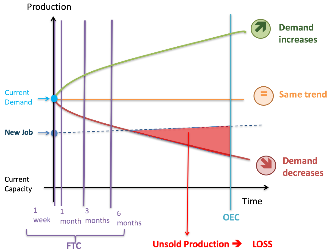
The central idea that governs job creation relies on the way the firm will estimate the future demand. If the demand is going to increase, a new job might be profitable, but not if there is a decrease in the demand. Hence, the firm will compute three scenarios – bad (noted \(\theta = -1\)), neutral (\(\theta = 0\)) and good (\(\theta = +1\)), which are depicted in Figure 2 below. We see in this figure that in the bad scenario, the demand of the firm is below its production with the new job after a certain time. As the firm cannot sell more than its demand, and the good is perishable, it may result in a loss because the firm has to continue to pay a salary if it is an OEC until economic dismissal is allowed (a year of delay in the reference experiment). In this example, we see that it may be more profitable for the firm to choose a contract with a shorter duration like a 3 months \(FTC\). Indeed, the firm will have the option to end this contract after 3 months in case of a bad scenario or to renew it if it goes well. \(FTC\) then acts as a buffer against the shocks on demand. However with a shorter contract it is more difficult to amortize the cost of hiring and training a new employee. It therefore appears a trade-off depending on how the employer perceives the risks. A supplementary trade-off comes from the increase of productivity with tenure in a job, that the employer anticipates. Since this productivity increase is shared by the employer, this factor also favors \(OEC\) and counterweights the risks of a dismissal cost.
Because of bounded rationality, the firms anticipate with finite horizons corresponding to the specifications of the different contract types. For each contract the decision process computes a net profit for each scenario, and then combines the three possible scenarios into a weighted profit. The weight of each scenario is calibrated at the aggregate level. The most profitable contract type and duration are selected (see Appendix A for details).
Job creations (step 1 in Figure 1)
The job creation proceeds in three steps:
- First, the firm checks if there is a sufficient demand margin to create a new job. Here it considers the actual (not anticipated) demand margin \(DM_{j,q,t}\) for firm \(j\) and occupation level \(q\) at time \(t\): if it exceeds the demand margin threshold \(DT\) (calibrated parameter), then the firm moves to the next step. Otherwise, no job is created.
- If there is in the firm a pending job in the occupation \(q\), the firm considers to hire a new person for this job (taking into account the eventual grace period). Therefore the pending job becomes a vacant job. Otherwise, it moves to the next step.
- Here, \(DM_{j,q,t} > DT\) and there are no pending jobs in occupation \(q\). Hence, the firm considers to create a new job \(p\) of the occupation \(q\). The characteristics of this new job are randomly drawn (cf. Section 2.6 above). From these job features, the firm must decide which type of contract suits better.
In order to create a job and choose a contract, the firm proceeds as follow:
- During a prospecting phase, the firm receives information about \(NPros\) job seekers of the occupation \(q\), who have applied to a job with a \(FTC\) and \(NPros\) job seekers of the occupation \(q\) who have applied to a job with a \(OEC\) during the last period. The expected profit per period \(\phi^{per}_{i,j,p,q,c, t}\) for a candidate \(i\) on a job \(p\) with a contract \(c\) is then computed for each contract (see Appendix A) : the \(OEC\) contract is compared with several \(FTC\) with different fixed terms (1 week, 1 month, 2 months, 6 months, 12 months, 18 months). As described in Appendix A, it takes into account the training costs for the job.
- Then the firm chooses to create the contract \(c\) with the best average positive profit, calculated along a set of potential candidates. These candidates are job seekers and the employer is informed via JobAds of their anticipated productivity level corresponding to their occupation, given their human capitals and the base production in the job (the information is based on equation 4 but the productivity kernel and the condition factor are unknown to the firm and set at their average). The employer will choose the contract \(c^*\) that gives the highest positive expected profit per period \(\phi^{per}_{i,j,p,q,c, t}\). If all the profits are negative, no new job is created.
- The firm continues to consider creating new jobs as long as \(DM_{j,q,t} > DT\).
Job destruction (step 2 in Figure 1)
By contrast, when there is a significant reduction in its demand in one occupation (in our model, this is when \(DM_{j,q,t}<-DT\)), the firm reacts in the short-term by removing its pending jobs and vacancies. In the medium run (on a yearly basis), if this low cost adjustment is not sufficient, the firm considers the possibility to dismiss workers.
Moreover, independently of the demand level, pending jobs and the vacancies that remain unfilled and have a duration greater than a fixed threshold – a parameter that will differ for \(FTC\) and \(OEC\) – are destroyed since they have a cost.
Economic dismissals: an evaluation of the financial viability of the company is performed on a yearly basis (52 periods in the simulation). The first date of the balance sheet is drawn randomly, then this financial reporting occurs every year from this date. The company calculates its yearly return that is computed as the ratio of the yearly profit over the total labor cost21. If this return falls below a certain profitability threshold (a fixed parameter \(PT\), that will be calibrated, but has to be negative, representing losses), the firm can justify an economic dismissal procedure. This is the formal implementation of our interpretation of the French jurisprudence (before the El-Khomri law) over the serious economic difficulties that allow to dismiss. However, owing to the diversity of judgments when workers appeal for unfair dismissal, an employer, even though she respects the threshold, may be condemned in industrial courts. Therefore she anticipates penalties on the base of the probabilities of litigation and loosing the case, which are added to the severance costs:
- all remaining vacancies are removed.
- after all the vacancies have been removed, if \(DM_{j,q,t}<-DT\) still holds, the firm considers dismissing employees. It selects one employee randomly, computes the associated profit \(\Phi^{tot}_{i,j,p,q,c, t}\) and the firing cost \(EFC\). If \(\Phi^{tot}_{i,j,p,q,c,t} < - EFC\) , the firm dismisses the employee. This process is repeated until \(DM_{j,q,t} > -DT\) or if all employees have been evaluated.
In the event that the company has a return below \(PT\) and has no employees to dismiss, the managing director "dismisses" himself, which in this case leads to the bankruptcy of the firm that is removed from the simulation. The managing director becomes unemployed. However, we want to keep the number of firms constant 22. Hence, when a bankruptcy has occurred, we randomly select an active agent in the simulation to create a new firm and manage it. He will be the only producer in the firm (until he starts to recruit).
Employee evaluations (step 3 in Figure 1)
In each period, the firm examines if some employees have to be evaluated. This individual evaluation may occur:
- At the end of the probationary period for \(FTC\) and \(OEC\);
- Every year, at the anniversary date of the contract, for \(OEC\) employee;
- At the end of \(FTC\) contract to decide if it should be renewed;
- At the end of \(FTC\) contract, if the transformation of \(FTC\) to \(OEC\) is to be considered.
Dismissal for personal reasons (insufficient productivity): the process takes two steps:
- First, the firm evaluates if there is a case for considering the dismissal. That could be the case if the employee’s production is below the firm’s requirement. Thus, there is a chance that the firm considers to fire this employee for personal reasons if the annual production of the employee \(Q_{i,j,p,q,t}^{eval}\) satisfies: \(Q_{i,j,p,q,t}^{eval}<\rho\times Q_{p,q}^{required}\) where \(Q_{p,q}^{required}\) is the required level of production and \(\rho\) an exogenous – calibrated – parameter in \([0.7,0.9]\). \(\rho\) encodes the tolerance the firm has with underproduction, or the maximum margin risk it accepts to take23
- Then the firm decides whether such a dismissal is more profitable or less costly than keeping him.
Hiring phase and promotions (step 7-8 in Figure 1)
Once the firm has chosen which contract \(c\) to create, a hiring norm must be computed to evaluate the candidates. This hiring norm is the profitability threshold below which it prefers to refuse a candidate. To do so, it uses the positive expected profits \(\Phi_{j,p,q,c,t}^{avg}\) calculated for each of the \(NPros\) candidates during the prospecting phasecomputes the average \(\Phi_{Moy}\), the minimum \(\Phi_{Min}\) and the maximum \(\Phi_{Max}\) values.
The hiring norm of the firm is given by the main economic factors taken into account in search theory:
| $$HNorm_{j,p,q,t=crea} = (\phi^{per}_{Moy} + N_1 \times (\phi^{per}_{Max}- \phi^{per}_{Min})) \frac{N(d_c)}{H(TIGH_{q,t=crea})} $$ | \[(9)\] |
- \(t=crea\) is the time of the creation of the contract.
- \(N_{1}\) is calibrated in \([0,1]\). The hiring norm increases with \(\phi^{per}_{Max}- \phi^{per}_{Min}\), so that the firm favors a large dispersion of candidates’ qualities in order to increase the probability to get better candidates, as prescribed by search theory.
- \(N(d_c) = N_2 + N_3 \times d_c\) , an increasing function24 of the duration of the contract \(d_{c}\) proposed for the job. \(N_2\) et \(N_3\) are two calibrated parameters in \([0,1]\) . We assume that the firm will be more demanding for longer contracts, as they imply to keep the employee for a longer time.
- \(TIGH_{q,t=crea}\) is the tightness on the labor market at the time of job creation and is given by \(TIGH_{q,t=crea}=\frac{V_{q,t}}{U_{q,t}}\) with \(V_{q,t}\) the vacancy rate and \(U_{q,t}\) the unemployment rate at time t for the occupation \(q\). The higher this tension, the more the firm has to lower its requirements if it hopes to find a candidate. We assume that the impact of the tension to \(HN\) is limited to \(\pm 20 \%\), because the hiring norm could be otherwise increased above the profitability of any worker, so \(H\) is a logistic function with values between 0.8 and 1.2 and given by \(H(x)=0.8+\frac{0.4}{1+20\times e^{-3x}}\).
This hiring norm above is then decreased by a percentage \(N_{4}\) in each period until the job is filled, but never drops below 0.
Hiring takes place in three steps:
- Receiving applications – The firm receives applications from external and internal applicants.
-
Selection and potential hiring
– A two-step process takes place:
- First, the firm computes a score for each candidate (internal or external), given by the expected profit per period \(\Phi_{i,j,p,q,c,t}^{per}\). Then the best candidate (highest score) is selected.
- Thereafter, the firm checks if this candidate’s score exceeds the hiring norm. If this is the case, the candidate is hired, otherwise, the job remains vacant.
- Internal promotion – If the best candidate hired is an internal candidate of the company, it is a promotion. The employee acquires the occupation level of the job.
When an individual is hired for the job, he is trained and receives the minimum required human capital for the job if he does not have it yet and the firm pays for it:
| $$\begin{aligned} HC_{i,t}^{gen} &\leftarrow \text{Max}(HC_{i,t}^{gen}, HC_{req,p}^{gen})\end{aligned}$$ | \[(10)\] |
| $$\begin{aligned}HC_{i,q,t}^{occ} &\leftarrow \text{Max}(HC_{i,q,t}^{occ}, HC_{req,q}^{occ})\end{aligned}$$ | \[(11)\] |
| $$\begin{aligned}HC_{i,p,t}^{spec} &\leftarrow \text{Max}(HC_{i,p,t}^{spec},HC_{req,p}^{spec})\end{aligned}$$ | \[(12)\] |
Individuals’ decisions (step 4-6 in Figure 1)
The individuals take decisions in each period of the simulation. This decision process is modeled with a state machine , where one individual, at each tick, will be in one particular state: inactive, unemployed, employed and not searching for another job, employed and seeking a new job, student or retired. The transitions between these states can be caused by individual choices (for example: to look for a job, to quit a job...), by external events (firing, death...), or eventually by a sequence of multiple decisions (e.g. applying for a job, and the firm hires the candidate).
Utility functions
Each individual uses a utility function, to decide whether he should stay in his current state or move to another one. The utility function has the generic form of a Cobb-Douglas function:
| $$U={(Income+Amenity+Stability)}^{1-\alpha}{(Free\ Time)}^{\alpha} $$ | \[(13)\] |
It is a weighted aggregation of four factors26 :
- Income: weekly income of the household in euros, divided by the number of consumption units (an adult counts for 1, a child 0.5, as often in consumers’studies). This specification means that we take into account that the partner’ earnings affect the participation decision of the individual. The family nature of the decisions is a fundamental element in labor economics and the theory of labor supply has studied the subject in depth. There are different theoretical possibilities. Models of joint decisions after bargaining inside the household rely on heavy assumptions and are uneasy to generalize to all other workers’ decisions on flows (such as quits). Our choice is in the line of Leuthold and Pollak as mentioned in the survey of family labor supply approaches by (Killingsworth & Heckman 1986). It is a very simple specification but it predicts some facts which are important both at a microeconomic level and at a macroeconomic level for WorkSim. First non wage incomes of the household affect the individual’s decisions, and notably the hours and the participation decision negatively in France, and the specification implies this result (Kabatek et al. 2014) . Secondly the partner’s earnings decrease in the model the individual’s participation probability. Kabatek et al. (2014) find this result also, which however remains debated (see (Briard 2017) for a survey of the empirical knowledge for the French case)27.
- Amenity: non-monetary features perceived by the individual (social recognition, working environment, job difficulty...). The factor is expressed as a percentage of the salary.
- Stability: criteria reflecting the preference of the individual for stability, i.e. for a job with the long contract duration. The maximum value is given for a permanent job ( \(OEC\) ). This stability is expressed as a percentage of the salary.
- Free time : free time per week available for the individual outside his working hours and search time. According to INSEE statistics28, we deduct 77 hours for sleep, eating, washing, from the total time per week. Then, the free time covers leisure but also caring for the children, and the model takes into account that the statistics show that women put more value on time for child care.
The parameter \(\alpha \in[0, 1]\) encodes the preference of the individual for free time against income, which depends, for a woman with young children, on the number of children. The INSEE statistics show that they still spend much more time than men on caring for children, and this is modeled as a higher "preference" for free time. A participation rate decreasing in the number of young children ensues.
Overview of the individuals’ decisions
The decision-making process of individuals is sequential and summed up in the state transition diagram depicted in Figure 3. At each period, the individual agent computes the utility of his current state and the utilities of each reachable state. Each utility is evaluated using the generic form given by Equation 13 above, and instantiated with the relevant values of income, amenity, stability and free time. Moreover, a factor \(ICHANG \in [1,2]\) is applied to several transitions to account for the psychological cost to do such a change (calibrated parameter). The higher \(ICHANG > 1\), the greater the new state utility must be to win the decision.
Job search process
After describing the different decision mechanisms, we now detail the overall job search process:
- Each period in the model, a job seeker spends time trying to get information on some jobs (wage, contract). JobAds sends a list of \(NV_{i,t}\) vacancies matching his occupation or a level above. We assume that these incoming job offers occur at a mean frequency that is known and independent of the time elapsed since the last offer. Therefore, we model the arrival of new job offers with a Poisson law: at time \(t\), this number of vacancies \(NV_{i,t}\) is drawn from a Poisson distribution with parameter \(\lambda_{t}=NSJ_{U} \times H(TIGH_{q,t})\), where \(NSJ_{U}\) is the average number of vacancies received by the unemployed at each period, and \(H\) is the same function of tightness as above. It can be the case that a job seeker does not obtain information on a single vacant job during the period.
-
The individual sends an application for the first offer whose utility is above his
reservation utility
\(UTRES_{i,t}\)29. If there is no job offer corresponding to his occupation or if all his applications are rejected, he lowers his reservation utility
\(UTRES_{i,t}\). Thus, at the end of each period, the reservation utility is updated :
where \(Ru_3 \in [0,0.005]\) is a calibrated parameter and \(Ru_4\) a fixed parameter (0.5). The first term of the equation accounts for the diminution with time in unemployment and the second is driven by a modification of \(UTUEM\), which is the utility for the unemployed (for instance a decrease of income will lower \(UTUEM\) and therefore \(UTRES\), as the urge to find the job increases). We do not set different reservation utilities for the two types of contracts since the workers search for the two types of jobs simultaneously. Yet, we take into account the lower return to search provided by the FTC in terms of utility since they offer shorter contracts, by including the stability parameter. This information is known to the searcher before contracting for an FTC. For an OEC the mean duration is known. This method ensures that searchers prefer OEC ceteris paribus, but may accept to apply to FTC when their research does not meet success by lowering their reservation utility30.$$\begin{aligned} UTRES_{i,t} = UTRES_{i,t-1} \times (1 - Ru_3) + Ru_4 \times (UTUEM_{i,t} - UTUEM_{i,t-1}) \end{aligned}$$ \[(14)\]
Demographic module (step 9-11 in Figure 1)
Household dynamics
In Worksim, an individual can be in three different household states:
- Child in a household, meaning that he stays with his parents. He can be in the labor market or not (when he is a student for example).
- Single person (with or without children).
- In couple (with or without children).
At each turn, the individuals change their household state according to transition probabilities deriving from real demographic data31 measured by the French national institute of statistics (INSEE).
A simulation evolves over time with a stable population, therefore the agents marry each other and have children that can enter later in the labor market. These children can leave their household in order to create a new household.
Retirements
The standard age of retirement is established to 65 in WorkSim, but an agent aged between 50 and 65 can get early retirement. We reproduce the share of retired individuals by age range according to INSEE statistics. Let us note however that a retired agent does not leave the simulation as he may still be a member of a household.
Aging
The age of an individual is increased by one week every tick or period of the simulation (one year corresponds to 52 ticks). The individuals leave definitely the simulation when they die at an age corresponding to the death rate by gender in France in 2014.
Validation process
The WorkSim methodology uses a validation process at two levels:
- model building: the way we design the model, and especially the agents’ decision rules is rooted as much as possible in empirical data and facts. Following the psychomimetism methodology (Kant 1999), we ensure that these decision processes do not violate the cognitive principles we build our model on (e.g. bounded rationality).
- data reproduction: we want our simulation to account for most available data on the labor market we aim to study. To do so, we use an automatic procedure to calibrate the model parameters for which we do not have an empirical value (see Calibration section below).
Calibration
Scaling
First of all, we must set the number of agents in the simulation. It must be large enough to account sufficiently for real behaviors, but not exceed our computational power32. For the experiments described below, we initialized the agents population from the real data found for year \(2014\), at a scale of \(1/4700\). We obtained 8713 individuals and 808 firm agents, for a total of 9521 agents in the simulation.
Calibration procedure
In order to calibrate the 56 parameters, we have to minimize a fitness function that is the weighted sum of the relative spreads between the outputs of our model and the real targets of the French labor market in 2014 (from multiple sources given by INSEE and DARES). We have chosen 63 targets grouped in 10 different categories : unemployment rates (7 targets), activity rates (6), salaries (14), job flows (12), FTC (4), long-term unemployment (3), mobility (between occupations (12), additional (part-time, vacancies, on-the-job searchers, training costs) (5). In most cases, we have a target per occupation or age range (see Appendix C).
To minimize this fitness function, we apply the evolutionary algorithm CMA-ES (Hansen & Ostermeier 2001), which is one of the most powerful algorithms to solve this kind of problem (Auger & Hansen 2012). CMA-ES means Covariance Matrix Adaptation Evolution Strategy. The principle of this evolutionary algorithm is to test step by step new generations of points in the parameters space. Each new generation of points is drawn stochastically according to the results obtained with the previous generation of points. The mean and the covariance matrix of the distribution of the new randomly drawn points are updated incrementally in order to move towards the best results obtained by previous generations.
At each iteration, the CMA-ES algorithm sets the values of all the 56 parameters. Then, to cope with the stochasticity we have in the model, 48 simulations are run (they are usually called replications in a calibration process) with a different seed for the random generator, and the outputs are averaged over these 48 simulations to obtain the fitness value of the iteration. We stop the calibration when the fitness does not improve (same minimum value) for 500 iterations.
Computational power needs
The calibration process is costly in terms of computational resources, because the total number of simulations can be quite high : it is given by the product of the number of iterations by the number of replications. With WorkSim, it took 2000 iterations to converge, and as stated above each iteration is made of 48 replications. Each replication takes about 1-2 minutes overall and the whole calibration process takes around two days to be completed on a processor with 48 cores.
Results of the calibration on the main targets
We obtain an average relative spread between all the outputs of our model and the real targets of 7.9 %. This can be deemed satisfactory for such a large non-linear model. We deal with a multi-objective optimization problem with many targets and parameters, and these problems are known to be hard to solve. The calibrated values of the parameters and the outputs of Worksim are shown in Appendix C (Tables 5 and 6 for the targets and Tables 7 and 8 for the parameters).
Results and Policy Experiments
In this section, we summarize the main results from a set of experiments we conducted with WorkSim. In this set, the model was calibrated to account for French data in 2014. Note that each experiment result is averaged over 200 simulations.
A brief characterization of the French Labor Market
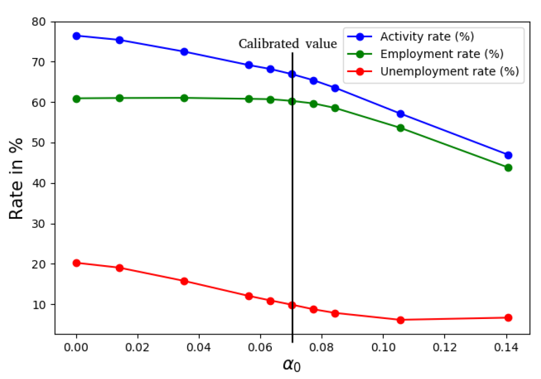
We first comment on some calibrated parameters. We do it briefly since most of them do not have known empirical counterparts (Tables 7 and 8). Several concern the labor supply and careers. In order to start to search for a job, the expected utility must be at least 26% higher than his present utility, a jump high enough to avoid repetitive moves between unemployment and inactivity. An unemployed starts losing human capital after 8 months, a delay which makes sense although data are missing. Then the rate of decrease is 0,93% per week, which appears a very high rate. The decline in reservation utility \(Ru_3\) is 20% per year of unemployment, a high rate, allowing for the acceptance by former OEC workers of FTC jobs after some time. However they are much more reluctant to look for jobs in the next lower broad occupation since it takes almost 4 years to accept this downgrading. The probability to look for a better occupation is higher at 1.4% per week. The wage careers are increasing and only slightly concave in general experience, since we do not consider the ceiling effect that obsolescence of human capital and illness or fatigue put on blue collars. However the managers do obtain a steeper career than intermediate level workers and blue-collars. Internal promotions from a broad occupation to another is low since it takes an average of 10 years. These figures are in agreement with the low social mobility in the French society in the XXIth century, compared to the previous century. On the employer’s side, a major parameter is the weight of the pessimistic scenario in the anticipation of demand. At 78.9%, it dominates the two other scenarios (neutral and optimistic), and means that the employers have a strong aversion to loss, which will deserve a sensitivity analysis below. Tolerance to a worker’s underproduction is fairly large at 80%, but within the bounds we have set. The parameter of the labor share in productivity \(\zeta\) may look very low at 29%, but the ratio concerns net wages and, if it is computed at the aggregate level in the model, it is higher since the workers at the minimum wage earn a higher share of their productivity, and then it matches the real French figure. Finally the profit threshold under which firms may layoff on economic grounds without too much legal risk PT is -22%, a loss, and clear evidence of serious economic difficulties .
The targets in Tables 5 and 6 are reasonably well fitted for our purpose. The unemployment rate and the activity rate are especially important for the model and well fitted. However the long term unemployment is under the targets, but it should be mentioned that the measure of unemployment tenure is given in the French labor force survey by the worker, who may forget very short contracts during a long spell of unemployment. The flows are also essential but difficult to calibrate since in our labor flows comprehensive system, they are interdependent and therefore determined by the complete set of behavioral parameters and legal constraints. The results can be deemed satisfactory. Economic layoffs are very low at 0.47% per year, since they are very costly in France before the ELK law, much lower than the layoffs for insufficient productivity, the exits at the end of the trial period, or the quit rate.
The model generates some important specific characteristics of the French Labor Market such as the very important share of FTC in terms of total entry flows, 80 %, and the contrasting fairly low figure of the share of the workers employed in such contracts: only 10%. The unemployment of the young is also much higher than the unemployment of the older workers. These results reproduce the known stylized facts of the French Labor Market, and the targets. These major stylised facts are not imposed by the assumptions of the model but emerge from the interactions of the agents during the simulation, given the calibration of the parameters on a large number of targets.
This confirms the dualism in the French Labor Market, which is displayed by the differences in the patterns of gross flows of the categories of workers. The model computes all the simulated flows, but allows for comparison with those which can be measured by the published statistics, and the results fit roughly. Most workers are stable in their OEC, while a minority undergoes short spells of employment in FTC and spells of unemployment between them. Moreover this dualism persists for a small proportion of young workers. The others obtain more stable OEC. It can be in the same firm in which they had an FTC through the experience (human capital) gained in FTC, as well as a screening process since the employers gather more precise information on their kernel productivity. This is a significant gross flow in the model. It can be through direct recruitment in OEC in other firms as the result of their increased experience.
Many more results are obtained, some of them novel in the sense that we simulate the entire gross flows matrix of labor while only some of the flows are documented in the statistics. They will not be detailed here, due to lack of space and the focus of the presentation of the results on the sensitivity of the main variables to the parameters, and on policy design.
Sensitivity analysis
In order to validate the mechanisms at play in the model, we undertake the sensitivity analysis of some important parameters. The sensitivity analysis consists in launching a set of simulations by changing each time the value of a parameter while the others remain at their calibrated value. For each point, we measure the outputs of the model after 104 periods (2 years) starting with the baseline calibrated model. We examine three types of parameters having a substantial impact on unemployment. First, we study the impact of a major parameter for individual’s choice: the base preference for free time. Secondly, we analyze a parameter playing an important role in unemployment theory and relating to workers’ behavior, the rate of decrease of the reservation utility with time spent in unemployment. These two parameters, being the workers’ choice, may have a considerable responsibility in unemployment. In a simple aggregate model, a preference of the workers for free time or a reluctance to accept jobs which are not so well paid (or not so stable) as the former job as time goes on, yield more unemployment. A systemic model like WorkSim may yield more nuanced results. Finally, we focus on one parameter affecting employers’s choices between the different contracts, relating to the formation of anticipations under uncertainty, a neglected topic in labor market models. The results reveal a huge impact on unemployment. This is in line with the focus of anticipations that macroeconomics now displays.
Preference for free time
The parameter \(\alpha_{0}\) represents the base mean preference for free time in the computation of the free time parameter \(\alpha\) (c.f. Section 2.9 above). The higher this parameter is, the more individuals prefer free time to labor incomes and the non-monetary characteristics of jobs (see Equation 13) of the utility function). As expected, an increase of \(\alpha_{0}\) , starting from the calibrated value, leads to a substantial decrease in the activity rate and the employment rate since individuals prefer free time (see Figure 4 below). For the unemployment rate, the expected move is less straightforward since it depends on the relative elasticities of the activity and employment rates to the preference for free time. The figure shows that the unemployment rate comes to a standstill. When \(\alpha_{0}\) decreases from the calibrated value, the activity rate increases, more individuals want to work, but most of these individuals do not find a job since total demand is fixed, so that we see an increase in the unemployment rate. To summarize the situation, the effects of a change in the preference for free time are asymmetric (starting from the calibrated value) as far as employment is concerned, bad if the change favors free time, and null if the change disfavors free time. This asymmetry shows that agent-based methodology uncovers nonlinear effects that standard aggregate models would not reveal.
Reservation utility decline with seniority in unemployment
In a model that embodies search behavior by the workers, the parameter \(Ru_3\) – entering in Equation 14) – plays a crucial role. It corresponds to the percentage of decline of reservation utility each week spent in unemployment. The higher the value of this parameter, the faster the reservation utility of unemployed decreases in the model. It represents the acceptance of unemployed to revise downwards the minimum utility at which they accept to work, as time elapses. Search theory makes two predictions. First, if the distribution of wages is known to the worker entering unemployment, and the rate of arrival of vacancies in which he would be selected, he should not lower his reservation wage. Secondly, if his household income falls unexpectedly over the spell of unemployment, he should lower his reservation wage. Concerning the first prediction, the elasticity of the reservation wage to unemployment seniority in Europe appears to be quite low, and in France, not significantly different from zero (Addison et al. 2009).
This study therefore appears to validate the first prediction of search theory. However, many studies show that workers, after being laid off, and recovering another job, are subject to a wage loss, which requires that they have lowered their reservation wage. We then considered that workers may be overoptimistic, not necessarily in terms of wages, but in terms of the possibility for them to access OEC. Since a worker learns about this difficulty over the spell by being not selected by employers, he accepts FTC more easily, which provide less stability. Since stability is a factor of the individual's utility in the model, this means that he decreases his reservation utility. We have then let the calibration decide over the rate of decline, which appears finally as non zero.
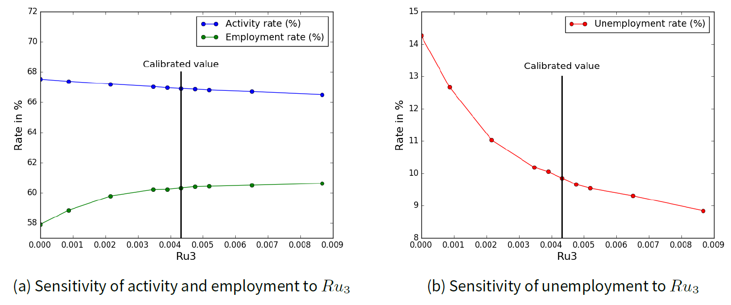
Figure 6 shows that the higher the decrease rate of the reservation utility, the lower the unemployment rate, since the unemployed revise faster their reservation utility and accept to apply to a higher number of job offers. When the reservation utility is rigid, search unemployment becomes a major component of total unemployment, the latter reaching 14% in the model. Such search unemployment is caused by the time that workers take to find a job that satisfies their requirements. It decreases when the reservation utility is more flexible with time elapsed in unemployment. The difference of 4 points in unemployment between the case in which reservation utility is rigid and the calibrated case could suggest that the behavior of unemployed is a major factor of unemployment. However we observe here a non linear effect: it would not decrease by more than one point if the rate of decline doubled beyond the calibrated case, so that a policy forcing unemployed to be less choosy would have a some effect. However it would not solve the unemployment problem, caused by a lack of demand and possibly by employers’ requirements as well as the minimum wage. Moreover the decrease in unemployment we can see on the right of Figure 6 is also due partly to a greater discouragement of the unemployed, because we observe a small decrease in the activity rate 5. When the reservation utility declines, at some level, it falls under the utility of inactivity, and triggers exit from unemployment. There are 122,000 discouraged workers for the highest rate of decline of the reservation utility. Finally the directions of the effects are clear but the sensitivity of unemployment to the rigidity (or flexibility) of the reservation utility to the time spent in unemployment should be lower on the real labor market, since the model underestimates the structural mismatches between supply and demand. We have only three broad occupations, hence very large labour segments, inside which only human capital, hiring norms of firms, and reservation utilities of workers matter for matching. Crafts or geography are not obstacles.
Sensitivity to the pessimistic scenario weight in demand anticipation
Employers form anticipations on the future of their own demand, based on past estimated trend and volatility. Bounded rationality leads them to consider only three scenarios, one neutral, meaning the trend remains the same, and two others, one with an upward deviation of 3 standard errors, and one with a downward deviation with 3 standard errors. They give weights to these scenarios which have asymmetric effects on profits since the bad scenario involves possible termination of OEC at a cost. The weights are calibrated and the value of the bad scenario \(\omega_{-1}\) is 78.9%. The domination of this scenario in the anticipations corresponds to an aversion to the loss (see Equation 24).
We then vary the coefficient \(\omega_{-1}\) , the other coefficients remain to their calibrated value and the three of them are re-normalized in order to make them sum to one. When \(\omega_{-1}\) increases, the employers reduce their hires on OEC in favor of more hires in FTC (Fig. 6a). Termination costs of OEC are so much higher than those undergone when having to pay an FTC until the end of his contract while he is producing in excess of demand. The employers also hire increasingly on short FTC of one week (Fig. 6d ), because these contracts are the least risky in case of future decline in demand. The role of buffer of the FTC against the uncertainty is then highlighted by this experiment.
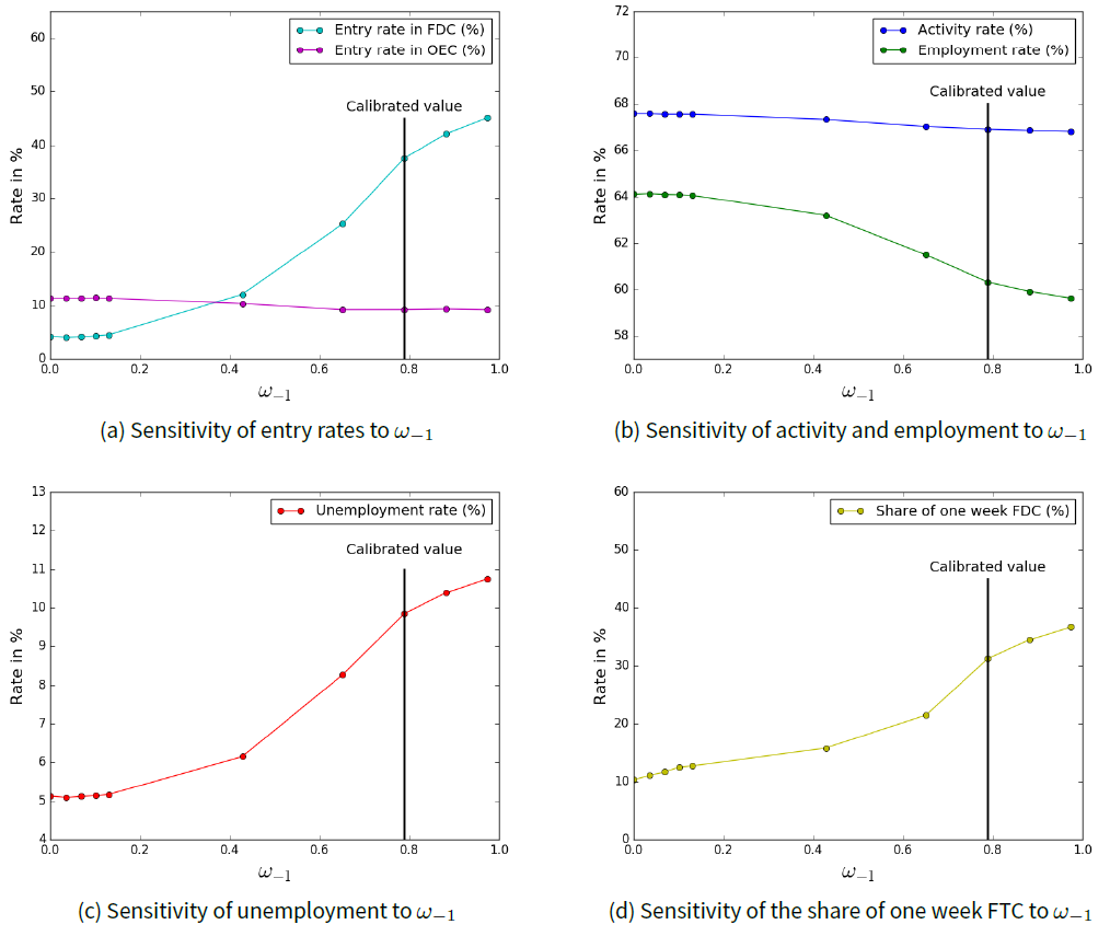
A reduction of this parameter could have a substantial impact on unemployment (Fig. 6d). In a hypothetical scenario, if it is set at the value of \(0\), the unemployment rate falls to the value of 5.13%. It highlights the importance to take into account psychological factors determining the employers’ behaviors in an economic model, as suggested by Keynes and recent Nobel prizes G. Akerlof and R. Shiller (Akerlof & Shiller 2009). These factors have a very strong impact on the choice of contract, FTC or OEC, and then on the functioning of the labor market.
The fact that companies are sensitive to uncertainty about demand helps explain how they will react to a change in labor market legislation, in particular with the ELK law (see the following section). The aversion to the risk of having to pay significant redundancy costs in the event of a fall in demand can limit part of the job creation with OEC contracts. With a softening of dismissal conditions, we therefore expect a higher rate of OEC contracts on the labor market.
Assessment of some labor public policies
We have conducted several simulation of labor policies, and since most of them had not been implemented at the time of the study, nothing was known on their effects at the moment of the decisions. In fact, one of the major purpose of WorkSim is to be a prototype for a generation of new models which advice policy decisions on employment and labor, by simulating them ex-ante and understanding the effects of one particular policy, or, better, joint policies. This requires structural model building because complex interactions occur.
Reduction of social charges
The level of social charges on employment is frequently discussed, especially by employers’ syndicates. In 2003, French Minister F. Fillon has passed a law that reduces the charges paid by the firms on wages, for salaries lower than 1.6 times the minimum wage (SMIC) 33. The decrease is 26 % for firms with 20 employees or more, and 28.1 % for the others. To study the effect of this policy, we compared the results of the baseline experiment34 with a new experiment in which these reductions of charges are removed. We measured a drop of 0.72 points in the unemployment rate, and a gain of 233,000 jobs, thanks to the reduction of charges. This result sets the gain within the range of the empirical studies on this policy, with between 200,000 to 400,000 jobs created or saved (Ourliac & Nouveau 2012). This experiment may be compared to ex post results has, beyond its intrinsic interest, the advantage of giving some validation to the model.
However, it might be more efficient to target the policy on lower wages. Therefore, we vary the maximum wage which can benefit from the policy, from 1.2 SMIC to 2.2 SMIC. The results are displayed in Table 1 below. It appears that the 1.2 SMIC target gives the most effective policy: the smallest unemployment rate ( \(9.55 \%\)), 298,000 more jobs, 253,000 fewer unemployed and also the lowest costs.
| Indicators | 1.2 SMIC | 1.3 SMIC | 1.6 SMIC | 2.2 SMIC |
|---|---|---|---|---|
| Unemployment rate (%) | 9.55 | 9.66 | 9.78 | 9.83 |
| Number of created jobs (in thousands) | 298 | 266 | 233 | 217 |
| Number of avoided unemployed (in thousands) | 253 | 228 | 192 | 180 |
| Gross cost per created jobs (in euros) | 86138 | 94361 | 110 729 | 119 816 |
| Gross cost per avoided unemployed (in euros) | 101 581 | 110 088 | 134 375 | 144 445 |
Variant with FTC renewable twice
We offer here a new experiment, by studying a policy formulated by the French government and adopted in June 2015 (Rebsamen Law, article 55). It relates to the possibility to renew an FTC twice, but always within the cumulative limit of 18 months. We still keep the assumption made in the model that the renewal of an FTC is of the same duration as the initial duration of the contract. In the evaluation of a new contract, it adds a new option to renew the FTC twice. Hence, the FTC has three potential durations : its initial duration, twice this duration (one renewal) and three times this duration (two renewals), always within the cumulative limit of 18 months.
The results of this variant are presented in Table 2. It appears that this policy raises the unemployment by 0.25 points, due to a stronger turnover effect of the workforce (+6.67 points). There are fewer entries in OEC (-0.66 points) and more entries in FTC (+7.08 points). It can be explained by the supplementary option of renewal making the FTC more attractive for the employers compared to OEC. In the simulation, the individuals in FTC are less likely to be hired in an OEC at the end of their first contract. This probability decreases from 15% to 14% because it becomes more beneficial for the employers to renew the contract, knowing that another renewal option remains possible in the future. However we observe that this policy lowers the share of long term unemployed (-1.4 points) by increasing the turnover rate on the labor market, hence recruitment. The objective of the government was to increase the flexibility of labor adjustment to demand change, but this seems to be at the cost of raising unemployment, ceteris paribus (aggregate demand being unchanged).
| Indicators | Reference | FTC renewable twice | Difference |
|---|---|---|---|
| Unemployment rate (%) | 9.78 | 10.03 | +0.25*** |
| Unemployment rate 15-24 yr (%) | 20.88 | 21.01 | +0.13*** |
| Unemployment rate 25-49 yr (%) | 8.4 | 8.72 | +0.32*** |
| Unemployment rate 50-64 yr (%) | 6.84 | 6.92 | +0.08 |
| Activity rate (%) | 66.93 | 66.82 | -0.11*** |
| Number of employed individuals (in thousands) | 24 629 | 25 519 | -110*** |
| Number of unemployed individuals (in thousands) | 2672 | 2737 | +65*** |
| Average net monthly wage | 2036 | 2041 | +5** |
| Long-term unemployment rate (%) | 34.6 | 33.2 | -1.4*** |
| Turnover rate (%) | 45.26 | 51.93 | +6.67*** |
| Average number of FTC spells | 1.97 | 2.2 | +0.23*** |
Evaluation of the facilitation of dismissals in the El Khomri Law
The El Khomri (name of the Minister of labor) law has been presented in March 2016 by the French government as the major labor law of François Hollande’s presidency. This law has set the war not only on the French political scene, but also between groups of highly recognized French economists such as Philippe Aghion, Olivier Blanchard, Jean Tirole, or Thomas Picketti and many others who have not hesitated to take a categorical position in favor or against it. Its final version was voted on July 21, 2016. There are many articles in the law, and several would be very difficult to implement in the model such as a much higher possibility to bargain within the firms for instance. Here we focus on the facilitation of the economic dismissals, considered as one of the main elements of the law, as it is likely to have an important impact on the labor market. The aim of the government was to encourage the employers to hire on OEC since dismissals would require less stringent but also more precisely defined economic conditions, hence less uncertainty on the industrial courts decisions in case of litigation and lower severance costs.
In the El Khomri Law (ELK), article 30, the conditions to allow economic dismissals are explicitly specified. The economic conditions and therefore the delay change. Economic dismissals are allowed in case of a decline either in the firm’s demand or its turnover, computed over a certain period of time, which depends on the firm’s size. For firms under 11 employees, the period is 1 quarter, for those between 11 and under 50 the period is 2 quarters, for firms between 50 and under 300, the period is 3 quarters, and for firms with 300 employees or more the period is 4 quarters. The law therefore softened the former conditions for economic dismissals, which implied that firms had to undergo serious economic difficulties to be allowed to fire. Let us keep in mind that we formalised in a simple and rough way the jurisprudence before the law as the requirement for firms to undergo losses during one year. However, even if respecting this condition, the employers could be taken to industrial courts. They could then be ordered to pay a much higher severance pay than computed by applying the regular indemnities by judges, if the latter estimated that the economic difficulties were not serious enough, or the legal procedures not perfectly respected (advance notice...), and the fires unjustified.
In the reference experiment without the law, we had integrated the anticipated supplementary costs, taking into account the probabilities to lose in courts, and the mean extra severance pay. For experiment with the ELK law, for the period after the ELK law was passed, we have modeled the new conditions and we have suppressed the litigation costs. The real data justify ex post this assumption since they show that the legal conflicts over fires have strongly declined since the law was passed. The French controversy indeed focused on the facilitation of dismissals, but more specifically on the decrease of the litigation risks. Aghion et al. (2016) supported the clearer conditions for dismissals and the consequent diminution in the litigation risk and costs as an incentive for the employers to hire on OEC, but did not mention adverse effects such as the increase of unemployment that faster adjustment to a decrease in firm own demand can generate. Both increases in hire and in economic fires are predicted by theoretical models of firing costs (see Bentolila et al. 2019), with no clear prediction on the net effect on unemployment. The empirical evidence is mixed (Boeri & others 2011). Askenazy et al. (2016) argued on theses bases that firing costs have not been proved to be a source of unemployment in Europe, that restrictive fiscal policy was the source of unemployment, and that FTC should be severely restricted to diminish the segmentation on the French labor market. Our model studies the French labor market as a complex system in which the El Khomri law modifies the rules of the game, and the results are more complex than in the quoted papers which are not based on models35.
Effects under a stable aggregate demand
To begin with, we simulate the ELK law for a steady state of the exogenous aggregate demand36. The ELK law yields effects which change over time after the introduction of the law. They evolve during the first 3 years to stabilize after 4 years. This comes from the fact that it takes time for the firing conditions to be filled even under the new law. The immense majority of French firms are small or very small, and it takes time for such firms to face a cumulated change large enough to be allowed by the new law to fire at least one employee. The results are displayed in Table 3.
The law has no aggregate effect on the unemployment rate or the employment rate. Hires on OEC increase to reach 28% but the rate of exit increases in an identical manner. This is in accord to the empirical results as mentioned. However the law has strong distributive effects. It is very favorable to the young (15-24), both in the short and the long run, with a decline in unemployment of 148,000 after 4 years (it drops over 5 points). The impact is not significant for the prime age class (25-49). After 2 years, there is a small decrease in unemployment (-53,000) and an increase in employment (+71,000). However after 4 years the law has no significant effect on this age class. Finally the seniors (50-65) undergo a substantial rise in unemployment (+101,000), rising from 6.6 to 8%, i.e. 1.4 points, and a decrease in employment (-121,000).
Moreover, the mobility on the labor market is found to change very deeply, and the nature of the labor market is then transformed:
- The share of FTC in the hires falls from 77% to 30%. The OEC becomes the dominant hiring contract.
- the hiring rate in OEC doubles, as predicted by economic analysis as a result of lower firing costs (Bentolila & Bertola 1990).
- The proportion of FTC in ongoing contracts falls from 8% to 2.3%, which makes it a minor contract in terms of employment share. There is a decrease of the mean duration (renewal not included) from 3.6 weeks to 1.9 weeks. This double change means that FTC are now mainly used by firms having a really bad future demand forecast and no requirement in training for these jobs.
- The entry rate in FTC falls to a quarter of its value before the law. Hence less training costs for job specific training are lost.
- The economic dismissal rate jumps from 0.6% to 19%, a major change in a French labor market which has been characterized by an extremely low and decreasing economic dismissal rate during the present century. The decreases in the uncertainty of the cost and the delay induce this explosion in the rate. This rise is predicted by economic analysis, but its rate is a surprise. The diminution of hoarding that the high firing delays induced raise the firms’ average benefits by 14%.
- As a consequence of higher dismissals, the OEC become shorter (the median duration of OEC falls from 4.8 to 2 years) and more precarious, as the probability to lose one’s job within a year jumps from 8.17 to 13.13 (+4.9 points, +60 % relative increase), and more frequent spells of unemployment for the OEC. This consequence seems to dominate the favourable effects and lead to a small decrease in average utility.
- The integration of the remaining FTC employees into OEC is improved since the increased turnover on OEC makes opportunities higher. This result has been also obtained in cross section studies which compare countries with different FTC rates (Bentolila et al. 2019).
| Indicators | Reference | ELK law | Difference |
|---|---|---|---|
| Unemployment rate (%) | 10.37 | 10.26 | ns |
| Unemployment rate 15-24 yr (%) | 27.75 | 21.89 | -5.86*** |
| Unemployment rate 25-49 yr (%) | 9.1 | 9.24 | ns |
| Unemployment rate 50-64 yr (%) | 6.62 | 8.03 | +1.41*** |
| Activity rate (%) | 70 | 70.16 | +0.16** |
| Number of employed individuals (in thousands) | 25 591 | 25681 | ns |
| Number of unemployed individuals (in thousands) | 2960 | 2937 | ns |
| Entry rate in OEC (%) | 11.88 | 28.24 | +16.36*** |
| Entry rate in FTC (%) | 40.95 | 12.45 | -28.51*** |
| Average individual’s utility | 229.2 | 222.72 | -6.48*** |
| Average weekly firm benefit (in euros) | 4133 | 4728 | +595*** |
| Long-term unemployment rate (%) | 34.72 | 33.26 | -1.47*** |
| Economic firing rate (%) | 0.61 | 19.55 | +18.94*** |
| Probability to loose one’s OEC within a year (%) | 8.17 | 13.13 | +4.86*** |
Two major conclusions can be drawn. First, a significant substitution of the young to the seniors takes place. Secondly the new adjustment rules on the OEC have the logical effect of making the FTC a much less useful flexibility tool for the employers except when demand expectations are very bad and no training required. A main objective of the law is then achieved: the FTC are no longer the mean to get around the dismissal costs of OEC. They serve the legal purpose for which they have been allowed, namely to buffer temporary increases in demand.
The explanation of the opposed effects over the young versus the other categories is simple. The young were much more often than the others in FTC (22% against 7.6% for the 25-49 and 4.9% for the seniors) and benefit from their fall. The effect is enhanced (in the model) by the two effects on the seniors. First these are mainly in OEC and the latter become much more precarious, so that many seniors are now fired. Second they are then unemployed and employers are reluctant to hire seniors on OEC when training for the job is required since the proximity of retirement makes amortization difficult37. Young compete seniors out. The effects of the ELK law then go much beyond the higher flexibility of OEC. The law raises the integration of the young into (more precarious) OEC, and this shows that the screening and experience enhancing roles of FTC before the ELK were not a sufficient factor of integration for the young. The consequence of the substitution of OEC to FTC, namely the substitution of young workers to seniors, who are penalised, has been overlooked by the non quantitative analysis of the ELK law we mentioned38.
Sensitivity of adjustment to aggregate demand
We now change aggregate demand exogeneously in order to examine if the ELK law influences the effect on unemployment differently. Figure 7 gives values after 2 years. It shows that the adjustment of the labor force is predicted to be more important after the law. First, when demand declines under its value in the reference experiment, economic dismissals are more important, the suppression of the hoarded labor is more complete, and unemployment rises more under El-Khomri’s law. The effect reaches 4 points if demand is to fall by 25%. Secondly when demand rises above the reference value, the employers hire more easily on OEC, and unemployment decreases more under ELK law. For a symmetric increase in demand the decrease is 2 points. The responses are not symmetric for large changes since if demand is very high, there always remains some search unemployment caused by workers who raise their reservation utility. This higher sensitivity to demand could be predicted, yet its importance could not be, since FTC were a substantial buffer before the law, but finally less effective than the reduction in dismissal delays for OEC.
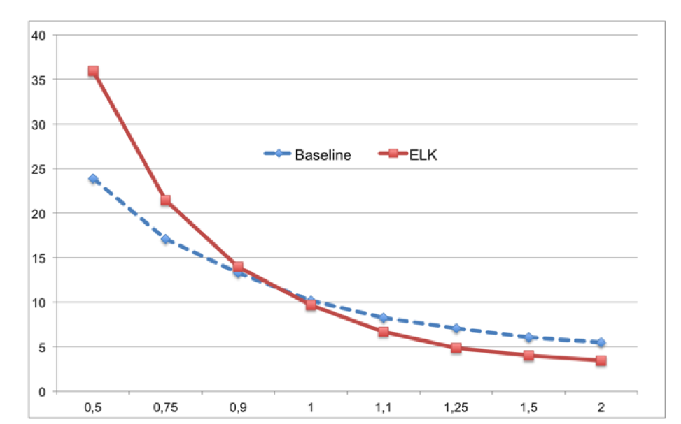
Discussion
In this synthetic paper, we present the WorkSim framework, a comprehensive model of the labor market. First the stock-flow accounting of individuals, based on gross flows, is complete and endogenous. It is supplemented by a stock-flow accounting of jobs for further analysis. The institutional environment is modeled and based on labor law, which sets constraints at the agent level on the possible decisions, taking into account the specific characteristics of each agent in his type, worker or employer. Therefore the simultaneous existence of unfavorable characteristics including the agent’s history may result in the exclusion of the labor market, a highly non linear effect that cannot be obtained in aggregate models in a realistic manner.
Secondly it implements numerous essential economic mechanisms that were not integrated before within a single labor market model: search on both sides of the market with multi-jobs firms, inter-temporal decision processes under bounded rationality, anticipations of demand shocks with risk aversion, learning, endogenous contract choices, endogenous salaries and productivities, different types of human capital. All are found to have major effects on activity, employment and unemployment.
Thirdly, WorkSim is calibrated on a large number of targets of the French labor market, by using a powerful evolutionary algorithm that has not already been used in economic models. On average and satisfactorily it reproduces these targets to conduct some economic analyses. Moreover, it reproduces the gross flows measured by different statistical sources and with different types of measures with a fairly satisfactory approximation. This gives us an estimation of the model accuracy, and is part of the model’s validation process.
Fourthly, we have conducted several analyzes and policy evaluations. These helped us to identify some core mechanisms in the French Labor Market: segmentation, screening and buffer roles of FTC, importance of employers’ loss aversion, among others. Each labor policy appears to have contrasting results for the different categories of workers in terms of employment improvements, benefits and costs. The complexity of the labor market has naturally led us to omit some more or less important institutions, and the number of targets remains small compared to this complexity. The effects of the policies should then be considered with the necessary scientific caution. The results are mainly meant to suggest new mechanisms, and the possibility of some effects of policies, which has not been highlighted before. One of the main conclusions is that institutions matter. Our agent-based model enabled us to simulate ex-ante effects of various policies, making it a precious tool to help policy design.
WorkSim in its present state has no equivalent in the agent-based models. These have macroeconomic goals that WorkSim does not have, and set assumptions on the labor market a minima. They mainly play with the wage setting mechanisms, comparing opposed theoretical assumptions such as wage rigidity versus flexibility, as our survey has shown (Dawid et al. 2012,2018, Dosi et al. 2020), and obtaining the standard macroeconomic stylised relations such as the Beveridge curve, the Phillips curve, and Okun’s curve. Devoided of a complete macroeconomic setting, WorkSim has not such goals. Those models who are closer in spirit to WorkSim as they are interested in the structure of the labor market, study specific mechanisms such as networks (Pingle & Tesfatsion 2004; Tassier & Menczer 2001). They have theoretical purposes and do not intend to model the mechanisms of a real labor market. Reproducing the main mechanisms of such a real market and their interactions requires a framework rich enough: an heterogenous population of individuals and households with a demographic module, the 3 main states (employment, unemployment, inactivity), the gross flows system, some main institutions like the different contracts, the minimum wage and benefits (and some others), some main constraints that labor law imposes, and finally, a calibration algorithm. The only agent-based models with such an agenda are our own previous models. ARTEMIS (Ballot 1981, 2002) presented such a model but was calibrated by hand. The first version of WorkSim was calibrated by the powerful algorithm CMA-ES that we described. Goudet et al. (2017) present the model, and Ballot et al. (2016) and Goudet et al. (2015) study policy experiments. In ARTEMIS and the first version of WorkSIm the choice between OEC and FTC was exogeneous39. The present paper provides a major improvement, by making the choice between permanent jobs (OEC) and temporary jobs (FTC) completely endogeneous.
Then the meaningful comparison is between WorkSim and the analytical search models of a dual labor market, which have gross flows between the employment and the unemployment states (the inactivity state is missing). Only one, (Cahuc et al. 2016), features a truly endogenous choice between OEC and FTC. The two models have at least two essential differences. There is first a fundamental conceptual difference between independent expected shocks on individual jobs in (Cahuc et al. 2016) and the global demand shock for a multi-jobs firm in WorkSim. The second difference lies in the types of costs when ending a job. In Cahuc et al. (2016), FTC cannot be extremely short because there is a cost of writing a contract. This cost is calibrated as 0.8 hour of production, significant enough to preclude extremely short contracts in the model. These would reduce to almost zero the possibility of a demand shock before they end, and could be repeated to compete out OEC.40 In fine an exogenous Poisson distribution of projects durations must determine the mix of contract types, if one repeats the draw for many jobs (the authors do not do this exercise). Our model considers firms which anticipate different evolutions of their total demand, weight them through risk aversion, and choose a mix of the two types of contracts: some FTC to avoid the risk of dismissing many OEC and paying advance notice and firing costs, but also OEC because FTC have also important drawbacks: they cannot amortise training costs on a short FTC, they cannot renew the incumbent more than once and undergo a waiting period before re-creating the job. Moreover the present mix of contracts is important for the choice in the dynamic context of the employer’s choice since it provides a low or high buffer according to the proportion of present FTC in the employment of the firm. Some results are common to the two models, namely the large ratio of FTC in hires, the lack of sensitivity of aggregate unemployment to firing costs, and the substitution of OEC to FTC if the firing cost is decreased. Yet WorkSim, which is also calibrated to a much larger number of targets than the Cahuc et al. (2016) 's model, can study in more depth the microeconomic and aggregate effects of the legal rules, as has been done with the ELK law, and previously with the generation contract in Ballot et al. (2016). It has also made possible to consider the heterogeneity of workers, and the divergent effects that a change in the rules induces on them, a fundamental topic when it comes to assess the effects of a policy on the young. This is not only a medium run phenomenon as it could appear in the present paper. Ballot et al. (2016) have been able to show that a cohort carries over its lifetime policy shocks undergone early, a result obtained by longitudinal studies (Schwandt & Von Wachter 2019), and a major topic since the Great Recession and the Covid.
Future directions
The model can be extended in several directions. Firstly we can add more labor market institutions and mechanisms: temporary employment agencies, social networks, and lifelong training for instance. We can also integrate more organizational elements, including more detailed competences and tasks based production functions, as well as the monitoring role of the hierarchy. Secondly, WorkSim would benefit from being plugged into an agent-based macro-economic framework, in order to have consumption, investment and financial effects as well (this is work in process). The outcomes on wages and profits have effects which in turn modify aggregate demand and employment. One way to look at this is to assume, as done in this paper, that they are second order effects, but this might not be true.
Thirdly, tools to help analyzing and explaining the simulations are still to be developed further: visualization (improving the graphical interface in WorkSim), analyses of the agents’ decisions, automatic classification of agents’ trajectories to study individuals’ careers (cohort analysis). Another issue is the link with micro-econometrics, to improve the agents’ measures of elasticities and enhance the validation process. Fourthly, if the current version of WorkSim is primarily designed to account for the French Labor Market, most of its components and mechanisms could be re-used to describe labor markets in other countries. The elements specific to the French institutions (labor law) can be adapted when dealing with another country.
Acknowledgments
We are grateful to the reviewers for their useful comments and suggestions which helped us to significantly improve the paper.Notes
- The main empirical methodology relies on transition probabilities with a frequency no smaller than at least one month. This deletes short term contracts.
- Figure 3 describes the main transitions processes.
- The OEC correspond to the Contrats à durée indéterminée (CDI) and the FTC correspond to the Contrats à durée déterminée (CDD) .
- FTC and other non regular employment are even more important in Spain, Portugal, and Netherlands, according to OECD data .
- Temporary help is the subject of a work in process (Ballot et al. 2017).
- The exact rules are in Appendix B.
- A previous version by Goudet et al. (2017) used an exogenous mix.
- This has consequences since a centralized labor market has different outcomes from a decentralized labor market. The real labor markets have some intermediaries such as Employment Agencies and temporary help firms, but they should be introduced in a decentralized environment with their specificities.
- The search concept is necessary to distinguish the two states of “unemployed” and “inactive” on the basis of rational (boundedly or not) decisions of agents. The unemployed looks for a job and the inactive does not. There is indeed a flow from unemployment to inactivity, because the value in terms of unemployment utility (expected gains from search minus time foregone) may become lower than the utility of inactivity (non wage income, welfare and free time). In that case, the individual stops search and becomes inactive. The reverse can occur. Search costs and not only non wage income influence the choice between inactivity, unemployment and employment. When an agent has decided to search, while on-the-job or as an unemployed, search concepts define stopping rules to be a candidate for a vacant job or not.
- For instance an employer, when hiring on an OEC, has more information on a worker with whom she has a FTC contract than on an external candidate, hence FTC can be a stepping stone for OEC.
- For evidence of the bias introduced by a matching function as a result of an employment policy, see (Neugart 2008).
- Bentolila et al. (2019) confirm this state of the research. They propose a simpler version of the Cahuc et al. (2016) paper. Several papers had proposed before models of this choice but either the choice is not fully endogenous, or they make assumptions much too far from the French rules to be useful to discuss here. Cahuc et al. (2016) offer a survey.
- Briard (2007) presents a typology of careers based on a large number of individual trajectories which suggests a persistent segmentation over the life cycle. Beffy et al. ( 2008) show by use of econometrics on transitions that around 5% of prime age population cannot get a stable job.
- This work has spurred an extension by Silva et al. (2012) to distinguish routine and non routine workers, and in a framework with unbiased technical progress, explain the rise of unemployment with a paradoxical rise in offered wages in some countries such as the US and Portugal.
- The managing director works full time for the firm, and at the three occupations. The director never leaves the firm, except to retire or when the firm goes bankrupt.
- Artifacts in multi-agent systems are the passive (non-proactive) entities providing the services and functions that make individual agents work together (Omicini et al. 2008), and must be distinguished from proactive autonomous entities like the individuals or the firms.
- \(\mathcal{N}(\mu,\sigma)\) denotes a normal law distribution, with mean \(\mu\) and standard deviation \(\sigma\).
- There are now many studies that support all these three types of human capitals (e.g., Kambourov & Manovskii 2009; Crook et al. 2011). It appears as covering better the heterogeneity of skills types than the traditional Beckerian dichotomy between general and firm specific human capitals, and it has important effects on the evaluation of the workers and their selection. For instance mobility between occupations is much less than between jobs in the same occupation, and promoting workers from one job to another may involve some training costs within a firm.
- The firm does not want to destroy the job, if there is still a potential demand margin for it, so it becomes a pending job. We have here an important feature of WorkSim: unlike other models, we distinguish the job and the contract, several employees (and therefore several contracts) may have occupied the same job since its creation.
- Using estimates of Phillips’s curves would be inappropriate in the context of an economy with fixed prices, and downward rigid incumbents’ wages.
- The labor cost represents here the capital funds the firm has to pay in advance. Hence, the return is the ratio of the profit over this capital.
- We keep the number of firms constant for two main reasons. First, we do not aim to model the determinants of firm creation, way too complex and out of the scope of WorkSim. Secondly, we are looking for a stationary state with a scale-up for year 2014, to apply and assess policies, and this will not be possible if the number of firms evolves constantly.
- This tolerance has necessarily a minimum, and a maximum < 1 to ensure a non-zero tolerance. Moreover, if \(\rho\) is too high, it will create a lot of dismissals and the firm will run a higher risk to face litigation and a higher risk to lose if it underestimated the real employee’s productivity.
- In absence of empirical data, we assumed this function to be linear.
- We assume that this training has no duration. One should have in mind that most training in firms is only a few hours.
- More precisely amenity and stability are “monetized” for the sake of adding up to income, a fairly standard procedure in economics, which could be justified by enquiries on the "wage reduction" that workers would accept to have more stability or more amenity. Then the "total income " obtained and free time have different weights in the utility function.
- The correlation appears for women in the econometric studies, even if the husband’s earnings are made endogenous. In our specification, the man’s decisions are also affected by his wife’s earnings. These may affect such variables as his reservation utility. Decisions of a partner then depend on the other partner’s status by an iterative process which fits well bounded rationality rather than a joint decision as in the game models of family labor supply. A transaction cost ICHANG avoids frequent changes that such an iterative process could induce.
- INSEE Statistics on physiological time in France in 2010 (https://www.insee.fr/fr/statistiques/1281050#titre-bloc-1).
- The concept of reservation utility (or of reservation wage) is an important concept in labor economics, and more specifically in search theory. It is the equivalent of the hiring norm, for the individual, as it represents the minimum level of utility (or wage) to make it acceptable to an agent. Most models use the reservation wage concept, but then the state inactive cannot be endogenous. In WorkSim, if the reservation utility falls below the utility given by the inactivity state, the unemployed stops search.
- \(Ru3\) is positive and calibrated on the basis of the French experience. More details are given in the section on the sensitivity experiment on \(Ru3\). \(Ru4\) is inspired by the evidence of the Addison et al. (2009)'s study that shows that reservation wages in France respond positively and very significantly to unemployment benefits. Since we consider reservation utility, the coefficient 0.5 reflects that its rise is less than the computed change in utilities, as all measures of elasticities show, and based on our ignorance on a precise value between 0 and 1.
- Population in France in 2014 (https://www.insee.fr/fr/statistiques/3137409).
- As we show below, the simulation itself does not take too much time and power to run. The critical point is the calibration as it has to launch thousands of simulations to reach an acceptable solution.
- These results are based on a past calibration of the model on year 2011, but there should not be qualitative changes with 2014.
- As noted above, the baseline experiment is performed with parameters set to their calibrated values. One must bear in mind that an experiment result is the average of 200 simulations.
- Our simulation has been done in April 2016 and presented in newspapers, workshops and working papers shortly after, and is therefore really ex ante (Gérard Ballot et al. 2016). One could object that in 2019 an econometric study of the effects of the El Khomri law could be undertaken. However the law was only implemented at the beginning of 2017, and the time series would be short. Moreover the main problem would be the elimination of the other shocks and employment policy changes that the economy has undergone since. At the level of the aggregate effects these obstacles may be overcome, but at the level of more disaggregated groups, where we find strong effects, it is more difficult. Finally, given the complexity of the topic, the two methodologies can be regarded as complementary tools when ex post.
- We used for the ELK experiment in 2016 a scale of 1/2300, half the one in more recent experiments, with a total number of 20,000 agents : 18,300 individuals and 1,700 firms.
- The bias against hiring seniors on OEC is very strong in France and statistical discrimination based on alleged risks of health problems, lower motivation, or less ability to cope with change add in employers’decisions to the training problem which is the only one we model.
- However a caveat on the magnitude of these substitution results is in order. We have assumed that any job can be an FTC or an OEC, even if we take into account that employers should be deterred from FTC when training costs are high. In the real world, some jobs require trust and/or long experience and cannot be FTC, so that substitution is overestimated in the model.
- However ARTEMIS has an exogeneous choice between primary and secondary jobs, both permanent, and and endogeneous choice between the former jobs and temporary help jobs
- Very short contracts, of a maximum of one day, represent a large part 30% of the FTC contracts in 2017 (DARES 2018). Moreover in some sectors they can be renewed indefinitely without a waiting period or any other cost under the name of customery FTC ( CDD d’usage in french). We have included these in WorkSim
- cf. the official web page of the French administration: "unemployment benefit for return-to-work assistance of a private employee" (https://www.service-public.fr/particuliers/vosdroits/F14860).
Appendix
Appendix A: Evaluation of the expected average profit per period
\(\phi^{per}_{i,j,p,q,c, t}\)
of an individual on a job
\(p\)
with a contract
\(c\)
[evalcontract]
The weekly profit of a candidate \(i\) on a job \(p\) , after \(d\) spent periods and for a scenario \(\theta\) of demand evolution is:
| $${\phi}_{i,j,p,q,t}(\theta, d) = P \times max(0,min \left( Q_{i,j,p,q,t}(d) , AD_{j,q,t}(\theta, d) \right)) - S_{i,j,p,q,t}(d) \times \text{SalC} $$ | \[(15)\] |
- \(AD_{j,q,t}(\theta,d)\) the anticipated demand margin in the qualification \(q\) after \(d\) periods in a scenario \(\theta\) of demand evolution and estimated at time \(t\) by the firm.
- \(Q_{i,j,p,q,t}(d)\) the anticipated productivity of the individual after \(d\) period on the job
- \(S_{i,j,p,q,t}(d)\) the anticipated salary of the individual after \(d\) period on the job and \(SalC\) the payroll charges (in %)
- \(P\) is the fixed exogenous price of the good (set to 1 in the simulations)
When summing this profit from the start of period \(d_{v}\) (expected vacancy duration) to the end of \(d_c\) ( expected duration of the contract) and applying the discount rate \(r\) , we get the total profit:
| $$\Phi_{i,j,p,q,c,t}(\theta, d_c) = { \left(\sum^{d_{c}}_{d=1}{\frac{{\phi}_{i,j,p,q,t}(\theta, d))}{(1+r)^{d + d_v}}} \right) - \frac{EndC_c(d_{c})}{(1+r)^{d_v + d_{c}}} } $$ | \[(16)\] |
Then, for a given evaluated contract \(c\) the firm chooses the best duration, that is the one that gives the highest profit:
| $$\Phi^{*}_{i,j,p,q,c,t}(\theta) = \max_{d_{option} \in D^{option}_{c,i}} {\Phi_{i,j,p,q,c,t}(\theta, d_{option})} $$ | \[(17)\] |
with \(D^{option}_{c,i}\) the set of possible durations with the contract \(c\) and an employee \(i\). For an FTC with an initial duration \(d_{FTC}\) and renewable once for a maximum period of 18 months (72 periods in our model), \(D^{option}_c = \{d_{FTC}, Min(2\times d_{FTC}, 72) \}\) . For an OEC, we assume that the firm estimates an average potential duration \(d^{learned}\) by learning. \(D^{option}_{c}=\{d^{learned}\}\). These possible durations \(D^{option}_{c}\) may be reduced by an expected retirement of the new employee. Then \(D^{option}_{c,i} = \{min(d, age_{retirement} - age_{i}),\ d \in D^{option}_c \}\).
The net profit per period for a contract \(c\) with a duration \(d_{c}\) in scenario \(\theta\) is:
| $$\Phi^{net}_{i,j,p,q,c,t}(\theta) = \Phi^{*}_{i,j,p,q,c,t}(\theta) -VC - TC,$$ | \[(18)\] |
with \(VC\) the vacancy cost required to open this position and \(TC\) the training costs, paid after \(d_v\)periods. \(VC\) is given by:
| $$VC = \sum_{d=1}^{d_v}\frac{Vac_{c,j,q,p}}{(1+r)^d},$$ | \[(19)\] |
with \(Vac_{c,j,q,p} = PrVac_c \times SH_{j,q}^{base} \times HpW_p\), where \(PrVac_c\) is the percentage of the vacancy cost for a contract \(c\) with respect to the base salary. These percentages, \(PrVac_{OEC}\) for OEC and \(PrVac_{FTC}\) for FTC, are calibrated parameters
The training costs \(TC\) is proportional to the amount of human capital that the firm must invest in the employee in order to reach the required levels of the job:
| $$TC = \frac{{TC}^{spec} + {TC}^{gen} + {TC}^{occ}}{(1+r)^{d_v}},$$ | \[(20)\] |
with
| $$\begin{aligned} {TC}^{spec} &= PTr^{spec} \times SH_{j,q}^{base} \times HpW_p \times \text{Max}(0,HC_{Req,p}^{spec}-HC_{i,p,t}^{spec})\end{aligned}$$ | \[(21)\] |
| $$\begin{aligned}{TC}^{gen} &= PTr^{gen} \times SH_{j,q}^{base} \times HpW_p \times \text{Max}(0,HC_{Req,p}^{gen} - HC_{i,t}^{gen})\end{aligned}$$ | \[(22)\] |
| $$\begin{aligned}{TC}^{occ} &= PTr^{occ} \times SH_{j,q}^{base} \times HpW_p \times \text{Max}(0,HC_{Req,p,q}^{occ} - HC_{i,q,t}^{occ}).\end{aligned}$$ | \[(23)\] |
\(PTr^{spec}\), \(PTr^{gen}\) and \(PTr^{occ}\) are calibrated scale parameters (human capitals are not measured in the same units).
Finally, the firm computes the final (total) profit as the weighed average profit for the 3 scenarios of demand \(\theta\in\{-1,0,1\}\):
| $$\Phi_{i,j,p,q,c,t}^{tot}=\omega_{-1}\times\Phi_{i,j,p,q,c,t}^{net}(\theta=-1)+\omega_{0}\times\Phi_{i,j,p,q,c,t}^{net}(\theta=0)+\omega_{+1}\times\Phi_{i,j,p,q,c,t}^{net}(\theta=+1),$$ | \[(24)\] |
with \(\omega_{-1}\) , \(\omega_{0}\) and \(\omega_{+1}\) the weighing coefficients of the firm for each of the 3 scenarios. \(\omega_{-1}+\omega_{0}+\omega_{+1}=1\). The values of these coefficients represent how much the firms are averse to loss during the evaluation process.
A profit per period is then computed: \(\phi^{per}_{i,j,p,q,c, t} = \frac{\Phi^{tot}_{i,j,p,q,c,t}}{d_{tot}} \label{eq:ProfitPer}\) with \(d_{tot}\) the average expected duration of the contract. When the algorithm is used to compare contracts with different duration for the same job, and choose a type of contract for this new job, it is repeated for a set of potential candidates.
Appendix B: Institutional Framework
Main contracts of the French labor law
There are two main types of contracts in France in 2014: fixed duration contracts (FTC) and open ended contracts (OEC).
The main FTC features implemented in WorkSim are:
- A maximum duration of 18 months, including the possibility to be renewed once.
- A small probationary period of one day per working week with a limit of 2 weeks, if the expected duration of the contract is below 6 months, and of a limit of 1 month, if the expected duration of the contract is over 6 months.
- A special allowance that the employer must pay at the end of the contract and corresponding to 10% of the total gross salary paid during the contract.
- An FTC cannot be broken without heavy penalties (paying the remaining salary part).
The main OEC features implemented in WorkSim are:
- No duration limit, except retirement.
- A probationary period of 2 months for blue collars, 3 months for middle level jobs and 4 months for managers.
- No termination costs if the employee is quitting.
-
Firing costs depending on employee salary and seniority:
- No firing costs if the employee seniority is below one year, but dismissals must respect the Labor law.
- After one year the firing costs correspond to a fifth of a monthly wage per year of seniority. The firing costs are increased by two fifteenth of a monthly wage per year of seniority after ten years (cf. French labor law L.1234 - 9, R.1234 - 2 et R.1234 - 4). The reference salary used to compute these firing costs is the maximum between the average gross salary of the last twelve months and the average salary of the last three months.
- In case of firing, a legal dismissal advance notice period has to be respected. It corresponds to one month, if the employee seniority is below two years, and two months otherwise.
Social policy
The main parameters of the French social policy in 2014 implemented in WorkSim are the following:
Welfare allowance: people become eligible for the French welfare allowance (RSA) if one of the following conditions is met:
- to be 25 years old or older.
- to be a lone parent with one or more children.
- to be 18 years old or older and have worked at least two years during the last three years.
The monthly amount of the RSA for a household with no activity income depends on the number of children and is given in the Table 4.
| Number of children | Single person | Couple |
|---|---|---|
| 0 | 499 | 764 |
| 1 | 749 | 917 |
| 2 | 899 | 1069 |
| 3 | 1098 | 1248 |
| 4 | 1298 | 1448 |
| 5 | 1498 | 1648 |
The children of the household in this evaluation must be 25 years old or lower and be at the actual charge of the individual (children that perceive no income in the model). For a household with an activity income, the welfare allowance is a complement of resources, if the revenues of activity are below a guaranteed minimum amount (not detailed here).
Unemployment benefit: an individual becomes eligible for unemployment benefits if all of the following conditions are met:
- he has been fired or he has completed a fixed duration contract.
- he is looking for a new job.
- he has worked 112 days (full time) in the 28 months preceding the end of the employment contract, if he is less than 50 years old, or 36 months before the end of the employment contract, if he is 50 years old or older.
An individual receives the unemployment benefits over a period of time corresponding to his contribution period with a maximum of 24 months, if he is less than 50 years old, or 36 months if he is more than 50 years old.
The calculation of the allowance received depends on an average reference salary received in the past twelve months. We refer the reader to the official website of the French administration for more details on the allowance evaluation41.
Legal work time: the legal work time per week for a full time job is 35 hours.
Retirement pension: in WorkSim the minimum retirement age for a full-rate pension is 65 years. The retirement pension is taken into account in the household utility evaluations. For the reason of simplicity in this work, we assume that this retirement pension is the same for all agents and equal to 75% of the average salary of the last 25 years for employees in the private sector and equal to 75% of the average salary of the last 6 months for employees in the public sector.
Minimum wage: the monthly net minimum wage for a full-time job (SMIC) is 1128.7 Euros in 2014.
Social security contributions: employers and employees have to pay social security contributions. In 2014, the percentage of the employer’s social security contributions on net wage is 54%. The percentage of the employee’s social security contributions on net wage is 28%. There is a reduction of employer’s charges at the SMIC level corresponding to 26% of the gross wage for firms with 20 employees or more and 28.1% of the gross wage for firms with less than 20 employees.
Appendix C: calibration of the model
Calibration targets and Worksim outputs
| Description | Target value | WorkSim output |
|---|---|---|
| Unemployment rate (%) | 9.2 | 9.79 |
| Unemployment rate 15-24 yr (%) | 22.0 | 20.8 |
| Unemployment rate 25-49 yr (%) | 8.4 | 8.4 |
| Unemployment rate 50-64 yr (%) | 6.3 | 6.9 |
| Unemployment rate blue collar/employee (%) | 11.35 | 10.82 |
| Unemployment rate middle level job (%) | 5.0 | 6.8 |
| Unemployment rate manager (%) | 3.8 | 4.7 |
| Activity rate men 15-24 yr (%) | 41.3 | 39.1 |
| Activity rate men 25-49 yr (%) | 94.4 | 95.3 |
| Activity rate men 50-64 yr (%) | 61.9 | 58.9 |
| Activity rate women 15-24 yr (%) | 61.9 | 58.9 |
| Activity rate women 25-49 yr (%) | 83.6 | 83.5 |
| Activity rate women 50-64 yr (%) | 54.6 | 49.5 |
| Average monthly salary - blue collar/employee 15-24 yr (euros) | 1336 | 1158 |
| Average monthly salary - blue collar/employee 25-49 yr (euros) | 1624 | 1416 |
| Average monthly salary - blue collar/employee 50-64 yr (euros) | 1724 | 1904 |
| Average monthly salary - middle level job 15-24 yr (euros) | 1603 | 1200 |
| Average monthly salary - middle level job 25-49 yr (euros) | 2143 | 1835 |
| Average monthly salary - middle level job 50-64 yr (euros) | 2496 | 2822 |
| Average monthly salary - manager 15-24 yr (euros) | 2079 | 1363 |
| Average monthly salary - manager 25-49 yr (euros) | 3558 | 2935 |
| Average monthly salary - manager 50-64 yr (euros) | 4485 | 4782 |
| Average monthly salary - first decile (euros) | 1201 | 1072 |
| Average monthly salary - first quartile (euros) | 1412 | 1223 |
| Average monthly salary - median (euros) | 1773 | 1608 |
| Average monthly salary - third quartile (euros) | 2380 | 2416 |
| Average monthly salary - ninth decile (euros) | 3349 | 3554 |
| Description | Target value | WorkSim output |
|---|---|---|
| Annual entry rate (%) | 51.0 | 46.1 |
| Annual entry rate in FTC (%) | 40.0 | 36.9 |
| Annual entry rate in OEC (%) | 11.1 | 9.2 |
| Annual entry rate 15-29 yr (%) | 115 | 88.2 |
| Annual entry rate 30-49 yr (%) | 36.6 | 35.6 |
| Annual entry rate 50-64 yr (%) | 23.7 | 30.1 |
| Annual exit rate (%) | 49.4 | 43.7 |
| Annual end of contract FTC (%) | 35.2 | 29.4 |
| Annual quit rate (%) | 6.5 | 5.5 |
| Annual layoff for eco. reasons rate (%) | 0.5 | 0.47 |
| annual layoff for other reasons rate (%) | 3.2 | 3.0 |
| Annual end of probationary period rate (%) | 2.0 | 2.3 |
| Long term unemployment (more than 1 yr) - 15-24 yr (%) | 28.4 | 26.9 |
| Long term unemployment (more than 1 yr) - 25-49 yr (%) | 41.9 | 35.3 |
| Long term unemployment (more than 1 yr) - 50-64 yr (%) | 57.8 | 49.0 |
| Share of FTC in employment (%) | 9.9 | 10.1 |
| Share of FTC of less than one week in hiring (%) | 54.9 | 31.4 |
| Share of FTC of less than one month in hiring (%) | 21.0 | 19.9 |
| Share of customary FTC in employment (%) | 0.99 | 1.2 |
| Share of employed on the job search (%) | 4.3 | 3.0 |
| Half-time job share in employment (%) | 17.9 | 21.0 |
| Average cost of specific training in euros | 300 | 75 |
| Average cost of global training in euros | 1300 | 1054 |
| Average number of vacant jobs in thousands | 800 | 761 |
| Share of blue collars/employees in age class 15-24 yr (%) | 62.7 | 62.0 |
| Share of middle level jobs in age class 15-24 yr (%) | 25.6 | 26.4 |
| Share of managers in age class 15-24 yr (%) | 11.7 | 11.6 |
| Share of blue collars/employees in age class 25-49 yr (%) | 51.1 | 50.6 |
| Share of middle level job in age class 25-49 yr (%) | 27.9 | 28.3 |
| Share of managers in age class 25-49 yr (%) | 21.0 | 21.1 |
| Share of blue collars/employees in age class 50-64 yr (%) | 53.0 | 50.9 |
| Share of middle level job in age class 50-64 yr (%) | 25.2 | 26.8 |
| Share of managers in age class 50-64 yr (%) | 21.8 | 22.3 |
| Annual internal promotion rate (%) | 1 | 0.7 |
| Annual external promotion rate (%) | 1 | 0.44 |
| Annual downgrading rate (%) | 1 | 0.8 |
Calibrated exogenous parameters involved in individual decisions
| Parameter | Description | Value |
|---|---|---|
| \(\alpha_0\) | Average base factor for individual preference for free time | 0.071 |
| \(\alpha_{old}\) | Increment of the factor for individual preference for free time every year | 0.108 |
| \(\alpha_{child}\) | Sensitivity parameter of the preference for free time to the number of children for women | 0.193 |
| \(\alpha_{yw}\) | Specific preference for free time for young women under 25 having children | 11.6 |
| \(\sigma_{ kernelProd}\) | Standard deviation of the individual productivity kernel | 0.193 |
| \(Txp\) | Time before loosing experience when unemployed (in weeks) | 33 |
| \(Lxp\) | Ratio of human capital loss every week after these \(Txp\) periods | 0.93% |
| \(\beta\) | Linear coefficient of production in general human capital | 0.00396 |
| \(\beta'\) | Quadratic coefficient of production in general human capital | \(6.42\times 10^{-7}\) |
| \(\beta_0\) | Linear coefficient of production in general human capital for blue collars | 0.00151 |
| \(\beta'_0\) | Quadratic coefficient of production in general human capital for blue collars | \(5.87 \times 10^{-7}\) |
| \(\beta_1\) | Linear coefficient of production in general human capital for middle level jobs | 0.0023 |
| \(\beta'_1\) | Quadratic coefficient of production in general human capital for middle level jobs | \(3.88 \times 10^{-9}\) |
| \(\beta_2\) | Linear coefficient of production in general human capital for managers | 0.00394 |
| \(\beta'_2\) | Quadratic coefficient of production in general human capital for managers | \(7.22 \times 10^{-8}\) |
| \(ICHANG\) | Psychological cost of starting to search for a job | 1.26 |
| \(Ru_1\) | Parameter entering in reservation utility initialization for unemployed | 0.99 |
| \(Ru_2\) | Parameter entering in reservation utility initialization for PARAE | 0.158 |
| \(Ru_3\) | Ratio of decline of reservation utility each week spent in unemployment or inactivity | 0.0043 |
| \(FailT\) | Time without job before downgrading occupation level (in weeks) | 191 |
| \(PrBQ\) | Probability to look for a job with a better occupation level during job search | 0.014 |
| \(\sigma_C\) | standard deviation of random factor entering in physical condition of the individual | 0.092 |
| \(ET\) | Employability threshold for an individual | 124 |
Calibrated exogenous parameters involved in firm decisions
| Parameter | Description | Value |
|---|---|---|
| \(\mu_0\) | Average base hourly production for blue collar jobs | 4.92 |
| \(\mu_1\) | Average base hourly production for middle level jobs | 5.53 |
| \(\mu_2\) | Average base hourly production for manager jobs | 6.88 |
| \(\zeta\) | Share of the base productivity value kept by the firm | 0.71 |
| \(PT\) | Profit ratio threshold | -0.22 |
| \(\mu_{\Psi_0}\) | Average demand share allocated to blue collar jobs | 33.5% |
| \(\mu_{\Psi_1}\) | Average demand share allocated to middle level jobs | 28.1% |
| \(\mu_{\Psi_2}\) | Average demand share allocated to manager jobs | 38.4% |
| \(\mu_{max}\) | Maximum of the demand trend factor | 0.0052 |
| \(\sigma_{\mu}\) | Standard deviation of the demand trend factor | 0.037 |
| \({\mu }_{alea}\) | Maximum of the demand volatility factor | 0.0020 |
| \(\sigma_{alea}\) | Standard deviation of the demand volatility factor | 0.0033 |
| \(PrMid\) | Probability of half time job | 0.287 |
| \(MaxHC_{req}^{gen}\) | Maximum of the general human capital units required for a job | 1517 |
| \(MaxHC_{occ}^{gen}\) | Maximum of the occupational human capital units required for a job | 8.5 |
| \(MaxHC_{occ}^{spec}\) | Maximum of the specific human capital units required for a job | 127 |
| \(PTr^{gen}\) | technical coefficient for training cost evaluation in general human capital | 0.117 |
| \(PTr^{occ}\) | technical coefficient for training cost evaluation in occupational human capital | 1.51 |
| \(PTr^{spec}\) | technical coefficient for training cost evaluation in job specific human capital | 0.0228 |
| \(\sigma_0\) | Standard deviation of base estimated productivity by the firm | 0.224 |
| \(\delta_{\sigma}\) | Decreasing factor of \(\sigma_0\) with seniority on the job | 0.0032 |
| \(\omega_{-1}\) | Weight of pessimistic scenario in firm profit evaluation | 78.9% |
| \(\omega_{0}\) | Weight of neutral scenario in firm profit evaluation | 14.5% |
| \(\omega_{+1}\) | Weight of optimistic scenario in firm profit evaluation | 6.56% |
| \(N_1\) | Parameter entering in hiring norm evaluation | 0.38 |
| \(N_2\) | Parameter entering in hiring norm evaluation | 0.017 |
| \(N_3\) | Parameter entering in hiring norm evaluation | \(4.73 \times 10^{-5}\) |
| \(N_4\) | Decreasing factor of hiring norm every week | 11.7% |
| \(Init_V\) | Share of demand allocated to vacancy creation at initialization | 0.113 |
| \(PrVac_{FTC}\) | Parameter entering in FTC vacancy cost evaluation | 0.784 |
| \(PrVac_{OEC}\) | Parameter entering in OEC vacancy cost evaluation | 5.7 |
| \(SenT\) | Required level of seniority for a promotion (in weeks) | 556 |
| \(DT\) | Demand threshold beyond which the creation of a post is considered | 413 |
| \(\rho\) | Tolerance of the employer to employee’s underproduction | 0.8 |
References
ACOSS. (2011). Les déclarations d’embauche entre 2000 et 2010 : Une évolution marquée par la progression des cdd de moins d’un mois. ACOSS Stat, 143.
ADDISON, J. T., Centeno, M., & Portugal, P. (2009). Do reservation wages really decline? Some international evidence on the determinants of reservation wages. Journal of Labor Research, 30(1), 1–8. [doi:10.1007/s12122-008-9057-y]
AGHION, P., Algan, Y., Bénassy-Quéré, A., Blanchard, O., Bourguignon, F., Cahuc, P., & others. (2016). Le projet de loi El Khomri représente une avancée pour les plus fragiles. Le Monde. 03 Mars 2016.
AKERLOF, G. A., & Shiller, R. J. (2009). Animal Spirits: How Human Psychology Drives the Economy, and Why It Matters for Global Capitalism. Princeton, NJ: Princeton University Press.
ASKENAZY, P., Bacache, M., Behaghel, L., Breda, T., Cagé, J., & others. (2016). La “loi travail” ne réduira pas le chômage. Le Monde. 08 Mars 2016.
AUGER, A., & Hansen, N. (2012). Addressing numerical black-box optimization: CMAE-ES. LION 6, January 16-20, Paris, France.
BALLOT, G. (1981). Marché du travail et dynamique de la répartition des revenus salariaux. Thèse Pour Le Doctorat d’Etat d’Economie, Université Paris X-Nanterre.
BALLOT, G. (2002). Modeling the labor market as an evolving institution: Model artemis. Journal of Economic Behavior and Organization, 49(1), 5177. [doi:10.1016/s0167-2681(02)00058-6]
BALLOT, G., Goudet, O., & Kant, J.-D. (2016). Le projet de loi el khomri modifie profondément le marché du travail sans améliorer l’emploi global. La Matinale Du Journal Le Monde (Internet), April 5.
BALLOT, G., Kant, J.-D., & Goudet, O. (2016). Un modèle multi-agent du marché du travail français, outil d’évaluation des politiques de l’emploi: L’exemple du contrat de génération. Revue Économique, 67(4), 733–771. [doi:10.3917/reco.674.0733]
BALLOT, G., Kant, J.-D., & Goudet, O. (2017). Introducing a temporary help agency in a labor market : A multi-agent model. 22nd annual Workshop on the Economic Science with Heterogeneous Interacting Agents (WEHIA 2017), Jun 2017, Milan, Italy.
BALLOT, G., & Taymaz, E. (1997). The dynamics of firms in a micro-to-macro model: The role of training, learning and innovation. Journal of Evolutionary Economics, 7(4), 435457. [doi:10.1007/s001910050052]
BARLET, M., Blanchet, D., & Le Barbanchon, T. (2009). Microsimulation et modèles d’agents; une approche alternative pour l’évaluation des politiques d’emploi. Economie et Statistique, 51–76. [doi:10.3406/estat.2009.8063]
BEFFY, M., Coudin, E., & Rathelot, R. (2008). Who is confronted to insecure labor market histories? Some evidence based on the french labor market transitions. Document de Travail G2008/10, Direction Des Etudes et Synthèses Economiques, INSEE.
BENTOLILA, S., & Bertola, G. (1990). Firing costs and labour demand: How bad is eurosclerosis? The Review of Economic Studies, 57(3), 381–402. [doi:10.2307/2298020]
BENTOLILA, S., Dolado, J. J., & Jimeno, J. F. (2019). Dual labour markets revisited (Nos. 12126). IZA Discussion Papers.
BERGMANN, B. R. (1974). 'A microsimulation of the macroeconomy with explicitly represented money flows.' In Sanford, S. (Ed.), Annals of Economic and Social Measurement, volume 3, number 3 (pp. 475–489). National Bureau of Economic Research, Inc.
BLANCHFLOWER, D. G., & Oswald, A. J. (1994). The Wage Curve. Cambridge, MA: MIT press.
BOERI, T., & others. (2011). 'Institutional reforms and dualism in European labor markets.' In Ashenfelter, O. & Card, D. (Eds.),Handbook of Labor Economics, 4(Part B). Amsterdam, Elsevier, pp. 1173–1236.
BRIARD, K. (2007). Profils types des salariés du secteur privé: Approche par une classification des carrières. La Documentation Française, 4, 59–85. [doi:10.3406/ecop.2007.7672]
BRIARD, K. (2017). L’élasticité de l’offre de travail des femmes: Repères méthodologiques et principaux résultats pour la france. Document d’études 210, Mai, DARES.
CAHUC, P., Charlot, O., & Malherbet, F. (2016). Explaining the spread of temporary jobs and its impact on labor turnover. International Economic Review, 57(2), 533–572. [doi:10.1111/iere.12167]
CROOK, T. R., Todd, S. Y., Combs, J. G., Woehr, D. J., & Ketchen, D. (2011). Does human capital matter? A meta-analysis of the relationship between human capital and firm performance. Journal of Applied Psychology, 96(3), 443–456. [doi:10.1037/a0022147]
DARES. (2018). CDD, CDI : Comment évoluent les embauches et les ruptures depuis 25 ans ? DARES Analyses, 26.
DAWID, H., Gemkow, S., Harting, P., & Neugart, M. (2012). Labor market integration policies and the convergence of regions: The role of skills and technology diffusion. Journal of Evolutionary Economics, 22, 543-562. [doi:10.1007/s00191-011-0245-1]
DAWID, H., Harting, P., & Neugart, M. (2018). Cohesion policy and inequality dynamics: Insights from a heterogeneous agents macroeconomic model. Journal of Economic Behavior & Organization, 150, 220–255. [doi:10.1016/j.jebo.2018.03.015]
DOSI, G., Fagiolo, G., & Roventini, A. (2010). Schumpeter meeting Keynes: A policy-friendly model of endogenous growth and business cycles. Journal of Economic Dynamics and Control, 34(9), 1748–1767. [doi:10.1016/j.jedc.2010.06.018]
DOSI, G., Pereira, M. C., Roventini, A., & Virgillito, M. E. (2020). The labour-augmented K+S model: A laboratory for the analysis of institutional and policy regimes. EconomiA, 21(2), 160-184. [doi:10.1016/j.econ.2019.03.002]
ELIASSON, G. (1977). Competition and market processes in a simulation model of the swedish economy. American Economic Review, 67(1), 277–281.
FAGIOLO, G., Dosi, G., & Gabriele, R. (2004). Matching, bargaining, and wage setting in an evolutionary model of labor market and output dynamics. Advances in Complex Systems, 7(02), 157–186. [doi:10.1142/s0219525904000135]
GOUDET, O., Kant, J.-D., & Ballot, G. (2015). Forbidding fixed duration contracts: Unfolding the opposing consequences with a multi-agent model of the french labor market. In Advances in Artificial Economics (pp. 151–167). Springer. [doi:10.1007/978-3-319-09578-3_13]
GOUDET, O., Kant, J.-D., & Ballot, G. (2017). WorkSim: A calibrated agent-based model of the labor market accounting for workers’ stocks and gross flows. Computational Economics, 50(1), 21–68. [doi:10.1007/s10614-016-9577-0]
GRILICHES, Z. (1969). Capital-skill complementarity. The Review of Economics and Statistics, 465–468. [doi:10.2307/1926439]
HANSEN, N., & Ostermeier, A. (2001). Completely derandomized self-adaptation in evolution strategies. Evolutionary Computation, 9(2), 159195. [doi:10.1162/106365601750190398]
KABATEK, J., Van Soest, A., & Stancanelli, E. (2014). Income taxation, labour supply and housework: A discrete choice model for french couples. Labour Economics, 27, 30–43.
KAMBOUROV, G., & Manovskii, I. (2009). Occupational specificity of human capital. International Economic Review, 50(1), 63–115. [doi:10.1111/j.1468-2354.2008.00524.x]
KANT, J.-D. (1999). Modeling human cognition with artificial systems : Some methodological considerations. Proceedings of Hcp 99 (Human Centered Processes), 501–508.
KILLINGSWORTH, M. R., & Heckman, J. J. (1986). 'Female labor supply: A survey.' In O. Ashenfelter and R. Layard (Eds.), Handbook of Labor Economics, 1, Amsterdam: Elsevier, pp. 103–204. [doi:10.1016/s1573-4463(86)01005-2]
KRAMARZ, F., Beffy, M., Buchinsky, M., Fougère, D., & Kamionka, T. (2006). The returns to seniority in France (and why are they lower than in the united states?). CEPR Discussion Paper. DP No 1935, January, IZA.
LE Barbanchon, T., & Malherbet, F. (2013). An anatomy of the french labour market: Country case study on labour market segmentation. ILO, Employment Analysis; Research Unit.
MARTINS, P. S., Solon, G., & Thomas, J. P. (2012). Measuring what employers do about entry wages over the business cycle: A new approach. American Economic Journal: Macroeconomics, 4(4), 36–55. [doi:10.1257/mac.4.4.36]
MORTENSEN, D., & Pissarides, C. (1994). Job creation and job destruction in the theory of unemployment. Review of Economic Studies, 61(3), 397415. [doi:10.2307/2297896]
NEUGART, M. (2008). Labor market policy evaluation with ACE. Journal of Economic Behavior and Organization, 67(2), 418–430. [doi:10.1016/j.jebo.2006.12.006]
NEUGART, M., & Richiardi, M. (2018). 'Agent-based models of the labor market.' In S.-h. Chen, M. Kaboudan, & Y.-R. Du (Eds.), The Oxford Handbook of Computational Economics and Finance (pp. 667–687). New York, NY: Oxford University Press. [doi:10.1093/oxfordhb/9780199844371.013.44]
NIJKAMP, P., & Poot, J. (2005). The last word on the wage curve? Journal of Economic Surveys, 19(3), 421–450. [doi:10.1111/j.0950-0804.2005.00254.x]
OMICINI, A., Ricci, A., & Viroli, M. (2008). Artifacts in the A & A meta-model for multi-agent systems. Autonomous Agents and Multi-Agent Systems, 17(3), 432–456. [doi:10.1007/s10458-008-9053-x]
OURLIAC, B., & Nouveau, C. (2012). Les allègements de cotisations sociales patronales sur les bas salaires en france de 1993 à 2009. Document d’études 169. DARES.
PHELPS, E. S., Alchian, A. A., Holt, C. C., & others. (1970). Microeconomic Foundations of Employment and Inflation Theory. W. W. Norton, New York.
PINGLE, M., & Tesfatsion, L. (2004). Evolution of worker-employer networks and behaviors under alternative non-employment benefits: An agent-based computational study.' In Leombruni, R. and Richiardi, M. (Eds.), Industry and labor dynamics: The agent-based computational economics approach (pp. 129–163). London: World Scientific. [doi:10.1142/9789812702258_0008]
REBITZER, J. B., & Taylor, L. J. (1991). A model of dual labor markets when product demand is uncertain. The Quarterly Journal of Economics, 106(4), 1373–1383. [doi:10.2307/2937969]
RICHIARDI, M. (2004). A search model of unemployment and firm dynamics. Advances in Complex Systems, 7(02), 203–221. [doi:10.1142/s0219525904000159]
SCHWANDT, H., & Von Wachter, T. (2019). Unlucky cohorts: Estimating the long-term effects of entering the labor market in a recession in large cross-sectional data sets. Journal of Labor Economics, 37(S1), S161–S198. [doi:10.3386/w25141]
SHAPIRO, C., & Stiglitz, J. E. (1984). Equilibrium unemployment as a worker discipline device. The American Economic Review, 74(3), 433–444.
SILVA, S. T., Valente, J. M., & Teixeira, A. A. (2012). An evolutionary model of industry dynamics and firms’ institutional behavior with job search, bargaining and matching. Journal of Economic Interaction and Coordination, 7(1), 23–61. [doi:10.1007/s11403-011-0085-y]
SIMON, H. A. (1956). Rational choice and the structure of the environment. Psychological Review, 63(2), 129–138.
TASSIER, T., & Menczer, F. (2001). Emerging small-world referral networks in evolutionary labor markets. Evolutionary Computation, IEEE Transactions on, 5(5), 482–492. [doi:10.1109/4235.956712]
THUROW, L. C. (1975). Generating Inequality. New York, NY: Basic books.
TVERSKY, A., & Kahneman, D. (1979). Prospect theory: An analysis of decision under risk. Econometrica, 47(2), 263–291.