
Introduction
Recently, fine wines have become a popular and viable alternative for investors interested in extensive portfolio diversification (Sanning et al. 2006; Masset & Henderson 2010; Masset & Weisskopf 2015), collectors willing to capture an emotional dividend (Dimson et al. 2015), or new consumers, particularly from emerging economies like China (Masset et al. 2016b). As a result, the major market indices (e.g., those disseminated by the Liv-ex exchange) more than tripled over 2000–2019, and the market size grew to around USD 5 billion per annum (Zimberoff 2018). Even more spectacular increases can be seen for particular producers and vintages: e.g., Lafite Rothschild 2000, whose ex-chateau price per bottle skyrocketed from 120 EUR to over 2250 EUR in 2011 (and levelled off at about 1250 EUR in early 2020). One of the key factors behind the increased attractiveness is the rapid development of trading infrastructure, which has transformed this hitherto opaque market into a more transparent, more efficient and global marketplace.
From the market microstructural perspective, several trading systems, in the meaning proposed by Domowitz & Lee (1998), are employed in the fine wine market, enabling order matching, transaction execution and pre- and post-trade data dissemination. Based on the classification used by The Fine Wine Market Liv-ex, we distinguish between three types of parallel trading systems: (a) auctions, (b) automated electronic trading (Liv-ex) and (c) bilateral over-the-counter agreements (OTC market). More precisely, auctions are considered an intermediated voice-based trading system or platform with an online bidding mechanism operated by auction providers, Liv-ex is an automated electronic trading system for exchange members, and the OTC market is a market for off-exchange trades where at least one party to the transaction is a Liv-ex member. In selecting the three venues, we follow the framework rooted in the theory of financial market microstructure (Madhavan 2000; De Jong & Rindi 2009). The terms trading venues, trading systems, markets, or market structures are used interchangeably (see Harris 2003). This division into trading venues allows for a more detailed look at market participant’s behaviour and various pricing mechanisms, such as one-sided auctions, two-sided auctions and bilateral bargaining. Although progressive trade automation has made several trading platforms gain importance by offering greater liquidity and cost-efficiency, the market remains fragmented with many parallel trading venues. The major venues include auctions (e.g., Sotheby’s, Christie’s), wine exchanges (e.g., Liv-ex, Cavex), online shopping sites (like eBay), or the over-the-counter (OTC) market. They differ in terms of the trading mechanisms, number of listed products and approved traders, trading rules, fee structures, transaction settlement, liquidity, or market transparency. Some of the venues are accessible for a broad spectrum of traders (e.g., wine auctions), while others limit access to the trading platform only to accredited traders (such as Liv-ex). Therefore, an investor must decide not only which wines to select to achieve the expected goals (such as the desired risk-return portfolio characteristics), but also which trading venue to operate on. At the same time, such fragmentation impedes price comparison and increases search costs.
In general, auctions, being a basic form of commerce, are widely used in the fine wine market, and auction data is commonly used in modelling fine wine prices (Storchmann 2012). Amidst numerous auction providers, a few firms play a prominent role, by offering bidding services via traditional salerooms, telephone connections or on- line platforms: for example, Sotheby’s, Christie’s, Acker Merrall and Condit, Hart Davis Hart, Zachys, Bonhams, Morell, Bloomsbury/Sokolin or Edward Roberts International (Cardebat et al. 2017; Czupryna & Oleksy 2018). These providers compete by using different fee structures. Commissions change over time and also vary de- pending on trade size, auction location and who is the trade initiator (buyer or seller). As revealed by Cardebat et al. (2017), during 2003–2012 buyer premiums ranged from 10% at Christie’s London to 23% at Acker Merrall New York, while seller commissions spanned from being equal to buyer premiums (as was the case at Christie’s London in 2003 and 2004) to being equal to zero (the case of Acker Merrall New York). In practice, auctions, particularly oral auctions, to some extent bear a resemblance to the open outcry systems in stock or commodity markets. Therefore, they can be categorised as a separate trading system offering broad and easy access to the market for both professional and non-professional traders.
The advent of automated and cost-effective electronic wine exchanges has been a milestone in ameliorating fine wine trading and improving price discovery in this market. Liv-ex exchange is one of the flagships in this field. It is a marketplace accessible for authorized professional wine traders, including negociants (wine merchants), brokers, retailers, importers, exporters, investment funds (so called ‘trading members’) and information seekers or researchers (so called ‘data members’). Besides trade matching and information dissemination, it provides comprehensive services in the field of wine storage and logistics. The price formation results from the trading dynamics of interacting buyer and seller interests. Orders can be placed anonymously (if preferred by traders) and order routing runs automatically. A continuous double auction mechanism is used to set prices. Three types of contracts are used: standard in bond (SIB), standard en primeur (SEP), and special (X). While SIB and SEP contracts define the physical condition of the wine and standard terms of trade (minimum lot size, tax status, payment, delivery conditions) for mature and en primeur fine wines respectively, X contracts pertain to wines which do not meet standard requirements (e.g. torn labels, signs of leakage, ripped or wrinkled capsules). For all sales and purchases, a standard 2% commission is charged. Members trading high volumes can lower trading costs by choosing various annual commission packages. Additionally, an annual membership fee (£1750 as at January 2017) and settlement fee (£3.5 per unit) complement the fee structure. When traders decide to store the stock in the Liv-ex UK warehouse for longer than three months, a storage fee (£0.55/month) or optional insurance fee (£10 + 0.015%) may be applicable. In practice, the Liv-ex trading system operates in the same way as the automated electronic trading systems in stock markets. Importantly, in contrast to other trading venues, the Liv-ex platform provides traders with information about wine prices formed in parallel on other markets, which allows them to compare prices directly without additional search costs.
Liv-ex members may carry out trading both on- and off-exchange. Trading off Liv-ex can be equated to trading in the OTC market, where dealers search for potential trading partners to execute bilateral trades directly. In contrast to stock markets, off-exchange trading in the fine wine market includes not only inter-dealer trades, but also sales to private clients. All this makes it a specific trading system with heterogeneous (professional and non-professional) traders and prices obtained from B2B or B2C trades. The information about the trader type, specifically the buyer, is unavailable, thus the proportion between professional and non-professional trades is unknown. While trading wines off-exchange, traders can set different prices depending on the search costs and relationships with the counterparty. The B2B trades are likely to produce smaller price premiums than B2C trades, due to the greater bargaining power of professional traders and possibly the greater transaction volumes they trade. The prices and profit margins in the OTC market also depend on trade location. For instance, according to the BinWise company[1], the wineries and vineyards in the US wine market have about 50% gross margin, distributors and wholesalers tend to have typically 28–30% gross margin, retailers around 30–50% and restaurants and bars around 70%. These levels can be further adjusted depending on the information asymmetry between traders, trade brokerages and trader motivations (profit-driven or utility-driven traders).
The inter-venue differences have been classically studied for financial assets (Barclay et al. 2006; Hendershott & Madhavan 2015) or commodities (Martinez et al. 2011; Banker et al. 2011). However, commodities markets, in particular wine markets, form a contrast to other financial markets. Firstly, wine markets are characterised by a larger number of different trading venues. Secondly, one observes higher heterogeneity of market participants and types of product on wine markets. In particular, wine market participants may have various motivations: immediate consumption, consumption at maturity or indefinite storage, compare (Dimson et al. 2015). All these factors may lead to higher differences in the prices observed across the different trading venues. On the other hand, studies for fine wine pricing across different trading venues are rarer (see Ashenfelter & Storchmann 2010; Dimson et al. 2015), and without reference to market microstructure theory. For instance, Ashenfelter & Storchmann (2010) show that the mean OTC prices, both for wholesale (6.19 UER per bottle) and retail (22.05 EUR per bottle) are significantly lower than for auctions (77.32 EUR per bottle), using the German wines dataset. However, these differences may be explained by different sample composition (wines of different quality are considered for each trading venue). Dimson et al. (2015) investigate the investment performance of Bordeaux First Class wines over their entire life cycle, with the use of two types of historical price records, namely, auction and retail list prices. The retail (OTC) prices were 0.07 — 0.50 GBP per bottle higher than the auction prices (depending on the model version used by the authors). Moreover, two different data sources, Christie’s for auction data and Berry Bros. & Rudd for retail prices, were used in their analysis. Our data encompassed 99,769 observations from the period of 2005–2015. The dataset was made available by the Liv-ex exchange and is normally available only to exchange members. In this respect, our research is based on a unique dataset that not only contains transactional data from three different trading venues but also applies to the same wines in a manner that ensures greater comparability due to one dataset provider. Firstly, this ensures the same way of collecting and cleaning data. Secondly, it restricts the OTC dataset to those transactions where the seller was an active Liv-ex member, thus rendering the Liv-ex and OTC data even more comparable.
In this study, we (1) examine how prices differ between the three trading venues: electronic trading (Liv-ex), auctions, and the OTC market; and (2) study the effects of microstructural assumptions on trading outcomes within a simulation model. The former reveals the relationships present in the actual transaction dataset; the latter shows which mechanisms are needed in the simulation model to reconstruct the findings. Our research also adds to the empirical literature on fine wine pricing in terms of research methodology. We combine econometric and simulation modelling, in order to deal with sparse and nonsynchronous data, which is a typical feature of fine wine as an illiquid asset (Masset et al. 2016a). The Bayesian approach has been selected for its flexibility, as a convenient alternative to the standard hedonic or repeat sale regressions that are commonly applied in modelling wine prices (Fogarty & Jones 2011; Cardebat et al. 2017; Masset & Weisskopf 2018). An agent-based model (ABM) was used to simulate the price formation. ABMs are frequently employed to reproduce the stylised facts on asset price formation in different trading systems and to elucidate their origin (Leal et al. 2016; Navarro & Larralde 2017). In the case of discretionary consumption goods, such as wines, the inclusion of consumer requirements and preferences (e.g., social emulation, innovation in consumption) is necessary to trigger the appropriate supply-side adaptations (Fernández-Márquez et al. 2017). In our model, we represent these elements by agents differing with respect to the private value of wine and deviations from the fundamental value.
The main findings of our paper are as follows. In the empirical data, we determine the mean price ranking (the OTC market being the most expensive and Liv-ex the least so; differing by about 4.5% and -0.8% from the auctions), detect a slight price decrease for larger transactions (approx. 0.3% reduction for a 10% volume increase) and some platykurtosis in price distribution (greatest in Liv-ex), and observe the most stochastic noise in auctions. In our multi-agent simulation, we show that trading mechanisms are insufficient for explaining the observed differences in prices across trading venues. We demonstrate that factoring in the differences in commission levels explains all of the observed price characteristics but one: an overly small price dispersion in the simulated OTC markets. This suggests that the real-world heterogeneity of local OTC markets is higher than the heterogeneity obtained by random assignment of the agents to the local markets in the simulation. The main reasons for this may lie in the differences in commission levels across the different local markets or in systematic differences between local markets in terms of the kind of participants who trade there. For example, some of the local markets may be characterised by relatively wealthy buyers.
The remainder of this paper is organised as follows. The empirical analysis is described in Section 2, while the agent-based model and simulation results are presented in Section 3. Section 4 contains a discussion of the study’s implications and limitations, alongside suggestions for future research. Supplementary details on the model are presented in the Appendix.
Bayesian Analysis of the Empirical Observations
Data structure
In our analysis, we used a unique dataset of fine wine prices from three different trading systems: an electronic trading system (Liv-ex), auctions and the OTC market. The database contains the transactional data covering a period from 2005 until the first quarter of 2015 (as the end date differs for various vintages, we used data up to the end of 2014). The data encompasses the five Bordeaux Premier Crus, with vintages starting from 1992. We only consider transactions with a typical bottle size of 750 ml, to exclude the effect of atypical bottle sizes on the price level. All data have been collected and provided by the Liv-ex exchange. Prices are quoted in pounds sterling, as it is the settlement currency at Liv-ex, and do not include any fees or taxes (net prices). Additionally, many prices needed to be converted from different currencies, which was done by Liv-ex using the exchange rates applicable on the date of the trades. Consequently, a small variation may occur between the trade dates and actual payments. From the perspective of our analysis, all wine prices are harmonised and thus fully comparable.
Model specification
The core of the model specification is how the transaction and market characteristics impact the final price. We assumed that there is an unobserved expected price for each producer/vintage combination, and this expected value changes proportionally with the Liv-ex 50 index. This assumption simplified the analysis, i.e. we did not have to model the price fluctuation path separately for each producer/vintage, which would introduce an abundance of degrees of freedom to the analysis and would be computationally too demanding. We believe that the prices of all the studied wines share a lot of common determinants, which can all be approximately summed up by the Liv-ex 50 index. The proportionality coefficient for a specific producer/vintage is denoted by \(\beta_{p,v}\), where \(p\) indexes the producer and \(v\) indexes the vintage.
The unobserved expected price is further adjusted in a single transaction to reflect the impact of the transaction characteristics, i.e. the amount sold and market type. More formally:
| $$\log(\textrm{EP}_w)=\log(\beta_{p,v} \times \textrm{index}_w) + E_\textrm{btl} \times \log(\textrm{btl}_w) + E_\textrm{OTC} \times \textrm{OTC}_w + E_\textrm{liv} \times \textrm{liv}_w,$$ | (1) |
We further assume that the price actually observed in a transaction depends on the expected price (as defined above) and is specific for each individual transaction, with some stochastic noise added to represent unmeasured factors, model misspecification, or actual randomness. More specifically, the price is treated as a random variable drawn from a symmetric distribution around the unobserved transaction-specific expected price, i.e. around \({\textrm{EP}_w}\). In the specification of this noise distribution, we accounted for two elements. Firstly, in order to reflect the possibility of a platykurtic distribution of prices, we assumed the final price to be a mixture (with equal probabilities) of two normal distributions with means \({\textrm{EP}} \times (1\pm \Delta_w)\), where \(\Delta_w\) depends on the market:
| $$\Delta_w=\Delta_\textrm{OTC} \times \textrm{OTC}_w + \Delta_\textrm{liv} \times \textrm{liv}_w + \Delta_\textrm{auc} \times \textrm{auc}_w$$ | (2) |
Secondly, to reflect the fact that we expect larger deviations of prices for more expensive wines, we assumed that the standard deviation (SD) of each of the two mixed normal distributions is proportional to the \(\textrm{EP}\), where the proportionality co-efficient also depends on the market (but SDs are identical for both distributions being mixed). Hence, SD is given as:
| $$\textrm{SD}_w=\textrm{EP} \times \left( \sigma_\textrm{OTC} \times \textrm{OTC}_w + \sigma_\textrm{liv} \times \textrm{liv}_w + \sigma_\textrm{auc} \times \textrm{auc}_w \right)$$ | (3) |
Model estimation
The model was specified in a Bayesian framework with non-informative priors (Kruschke 2014). The posterior distributions were estimated with Markov Chain Monte Carlo in the JAGS/R environment. In the simulation, consisting of 2,000 adaptations, 20,000 burnins and 10,000 iterations, four chains were used with random initial values. Medians of the posterior distributions were used as point estimates, and 2.5% and 97.5% percentiles were used to construct the 95% credible intervals (95%CIs). The model convergence was tested with PSRF statistics (no problems were identified).
Results
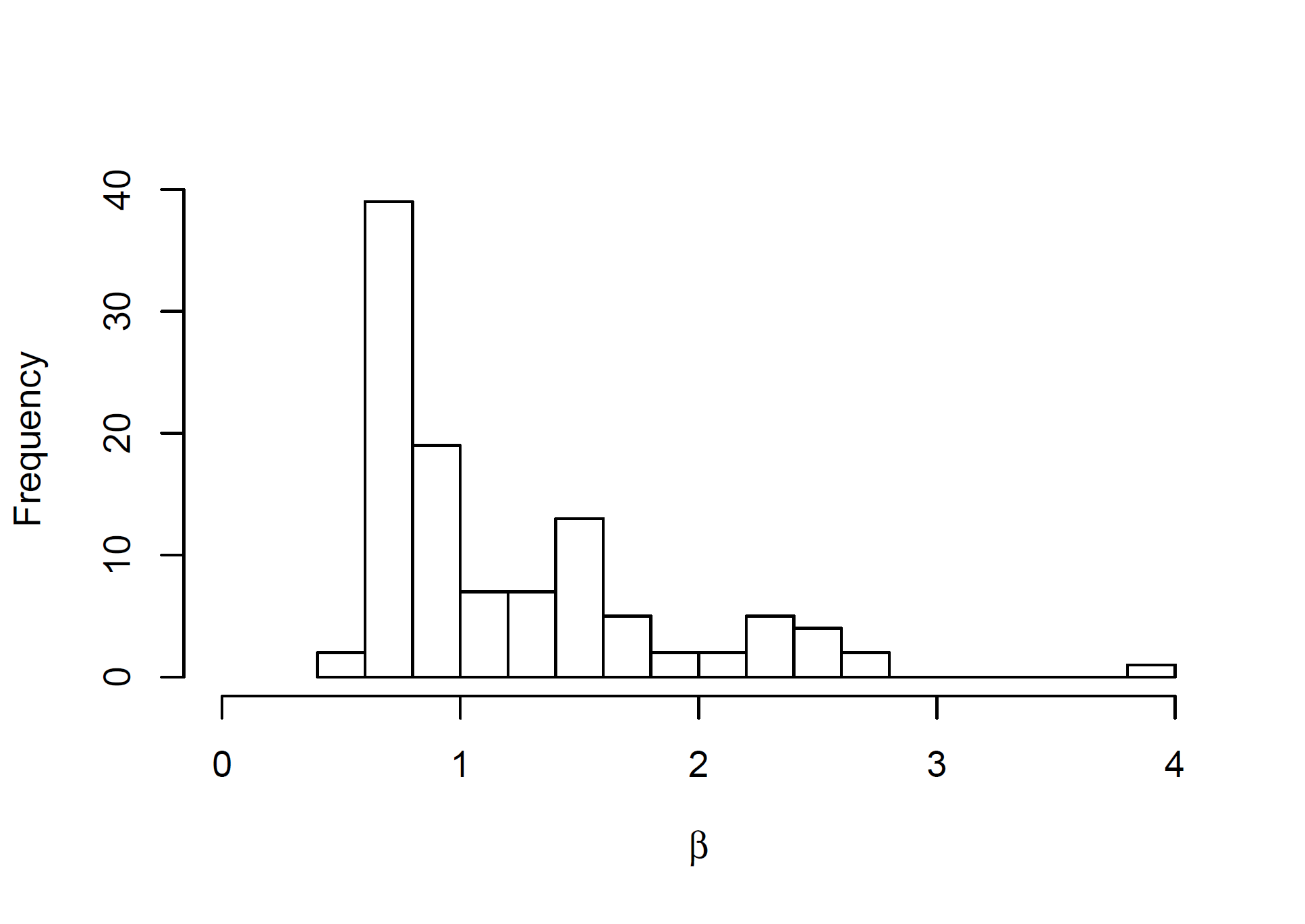
The results of the \(\beta\) parameters estimation are presented in Figure 1. The distribution is heavily right-skewed (skewness = 1.52), i.e. the majority of wines are valued less than the index, and exceptional ones can be valued much higher (the logarithms are also right-skewed, skewness = 0.67). The most expensive wine was Lafite Rothschild, vintage 2000, with its \(\beta\) amounting to 3.93.
The estimated values of other parameters are presented in Table 1. Increasing the size of the transaction lowers the price, with elasticity being estimated at -0.0313, i.e. we expect the value to be 5.5% lower on average if six bottles are traded (instead of one bottle), and 7.5% lower if a dozen are traded. The prices are 4.5% higher on average in the OTC market and 0.8% lower in the Liv-ex trading system (with the Auctions category serving as a benchmark). We found some platykurtosis, with all \(\Delta\) parameters being positive but close to 0 (with 95%CI touching 0). The largest \(\Delta\) was found for Liv-ex, which nicely coincides with intuition: in this exchange the offers can be made by either side (i.e. sellers or buyers), so we expect the prices to be more flatly distributed around the expected price, depending on the initiating side.
| Parameter | Point estimate | 95% CI |
| \(E_\textrm{btl}\) | -0.0313 | (-0.033; -0.0297) |
| \(E_\textrm{OTC}\) | 0.0441 | (0.0405; 0.0477) |
| \(E_\textrm{liv}\) | 0.0081 | (-0.0122; -0.0040) |
| \(\Delta_\textrm{OTC}\) | 0.0027 | (0.0000; 0.0064) |
| \(\Delta_\textrm{liv}\) | 0.0122 | (0.0000; 0.0274) |
| \(\Delta_\textrm{auc}\) | 0.0059 | (0.0000; 0.0145) |
| \(\sigma_\textrm{OTC}\) | 0.1871 | (0.1859; 0.1884) |
| \(\sigma_\textrm{liv}\) | 0.1520 | (0.1493; 0.1543) |
| \(\sigma_\textrm{auc}\) | 0.2732 | (0.2710; 0.2756) |
Finally, we found large differences between the markets in terms of the size of the deviation of the transaction price around the mean (the unobserved value). We found the smallest deviations in the Liv-ex market and the largest in Auctions (being approximately twice the size). In terms of these deviations, the OTC market is more similar to Liv-ex than to Auctions.
In the next section, we attempt to reconstruct the above findings within a simulation model, to see which mechanisms need to be implemented for it to succeed.
Agent-Based Approach
In our model, we consider wine producers who are only concerned about selling wine, and consumers who are interested in buying and subsequently drinking it. We consider a separate sub-model for each trading venue. Additionally, in the Appendix, there are two supplementary models (one for auctions and one for Liv-ex) shown for consideration, containing agents that are primarily interested in the active trading of wine (understood as profit-motivated purchasing and subsequent resale).
Agent-based model assumptions
Agents
We consider two types of agents: buyers and sellers, and three trading mechanisms (venues). In the first round, there are \(N_B\) buyers and \(N_S\) sellers, and each seller is endowed with one bottle of wine. For simplicity, we consider only one brand of wine (defined by a vintage and a producer). An agent is exogenously assigned to only one of the trading venues. As a consequence, an agent can trade with just one brand of wine and on one given trading venue.
Each agent, \(i\), has a private value of wine, \(v^i\). This can be the buy or sell value, depending on agent type. A Gaussian distribution of the private values among both buyers and sellers is assumed, with two parameter sets: \((\mu_B,\sigma_B) \) and \((\mu_S,\sigma_S)\), respectively. The parameters define the percentage difference from the fundamental value. On average, the buy value is higher than the fundamental value and the sell value is lower than the fundamental value. The private buy values can be interpreted as willingness-to-pay, whereas private sell values may be seen as the production cost plus a mark-up (see Hamill & Gilbert 2016). Different values for the averages of private buy/sell values are used for two reasons: firstly, to allow transactions to take place (buyers must be willing to pay more than sellers require); secondly, to reflect the platykurtic distribution, as described in the section on Bayesian modelling (the \(\Delta\) parameters).
In each run, we model 20 years of trading (the approximate time that Bordeaux premier cru wines are actively traded after production) with monthly observations, i.e. 240 individual rounds. In each round, every trader can engage in the act of wine exchange with probability \(\lambda_P\). Every trader who had made an earlier offer that was not accepted can withdraw this offer with probability \(\lambda_W\). Additionally, we model the removal from the market of a wine that remains uexchanged (e.g., owing to damage or the wine being consumed by the seller): in every round, each bottle is removed with probability \(\lambda_I\) (and the owner withdraws from the market).
Additionally, for each venue there is a commission level, \(c_l\). Based on this level and the private wine value, agents set their buy (\(p_b\)) and sell (\(p_s\)) prices according to the formulae defined in Equations 4 and 5. For the OTC market, the commission level \(c_l\) for buyers equals zero. We consider the net prices (and not the final prices) in our model and any commission due must be paid additionally by the buyer and seller.
| $$p^i_b=\frac{v^i}{1+c_l} $$ | (4) |
| $$p^i_s=\frac{v^i}{1-c_l}$$ | (5) |
Trading mechanisms
The Liv-ex market is modelled as a double-sided continuous auction (O’hara 1997; Hasbrouck 2007). In the case of Liv-ex, in each round every agent attempts with probability \(\lambda_P\) to place a limit order: an ask — a sell order in the case of sellers (an agent has a bottle of wine to sell), and a bid — a buy order in the case of buyers (an agent wants to buy and then consume a bottle of wine). Such an order specifies a sell price (the lowest price at which an agent is willing to sell) or a buy price (the highest price an agent is willing to pay for a wine order). Once an order is placed, we first verify whether there is a matching opposite limit order in the order book (the set of current outstanding buy and order limits). To be more precise, for a buyer we look for a sell order with the sell price lower or equal to the buy price, and for a seller we look for a buy order with the buy price higher or equal to the sell price. If there is a match, the transaction happens at the best price of the all matching orders. The best price is defined as the highest price for the buy orders and the lowest price for sell orders. Otherwise, buyer (seller) places a limit buy (sell) order with a limit equal to his/her buy (sell) price on the market. Such an order is added to the current order book. In each round, a trader can withdraw his/her existing order with probability \(\lambda_W\) .
In the case of the OTC market, we consider \(N_O\) different locations. Sellers and buyers are randomly allocated to locations at the beginning of the simulation (each agent to just one location). At each location, a wine is offered at an equilibrium price, calculated as follows. We first construct a demand and a supply curve by price-sorting the buyers and sellers in descending and ascending order, respectively. Where the curves intersect determines the equilibrium price, as in a classical microeconomic theory (see Mas-Colell et al. 1995), for example. More precisely, we look for the highest value of the variable \(n\) such that the buy price of the \(n\)th buyer is lower than or equal to the sell price of the \(n\)th seller. If we can find such an \(n\), the equilibrium price is set to the mean value of the buy price of the \(n\)th buyer and the sell price of the \(n\)th seller. Otherwise, it is set to the sell price of the \(1\)st seller - the one with the lowest sell price. In each round, a buyer tries to buy with probability \(\lambda_P\) and succeeds if his/her buy price is higher than or equal to the equilibrium price at this location. A seller is matched randomly (we assume that all bottles available in a particular shop[2] are for sale and are indistinguishable). The transaction price is set to the equilibrium price. After each successful transaction, the equilibrium price is recalculated. We do not allow for order withdrawal, as it is very rare in the case of OTC markets.
We model an auction market as an English auction (Mas-Colell et al. 1995). We consider \(N_A\) different locations, with each buyer and seller assigned to only one location (auction house). In each round, buyers and sellers may join an auction with probability \(\lambda_P\). Firstly, the sellers are ordered randomly and the buyers are ordered according to the buy price in ascending order. Wine bottles are offered for sale one by one, with the starting price set to half of the value of the seller’s asking price. A transaction takes place if the buy price of the last buyer (the one with the highest buy price of all other buyers) is higher than or equal to the starting price of the currently offered wine. The transaction price is the maximum of the starting price and the buy price of the buyer having the second highest buy price. We also do not allow for order withdrawal, as it is not possible in the case of auctions.
Simulation parameters
We ran the model separately for each venue. The ranges for the parameters determining agent behaviour are shown in Table 2. Furthermore, to systematically search the parameter space, we used 1000 value sets determined by Sobol numbers (Bratley & Fox 1988; Christophe & Petr 2014). For the parameters that are not directly observable and thus unknown (e.g., \(\mu_B\), \(\sigma_B\), \(\mu_S\), and \(\sigma_S\), which define the private wine value of the agents), we arbitrarily selected wide ranges. For the observable parameters, the ranges were set according to empirical data. The number of auction houses \(N_l^a\) or the inactivation probability \(\lambda_I\), which correspond to the assumed number of 240 rounds, are examples of such variables. We ran 16 simulations for each parameter set with different seeds, which led to 48000 = 3 \(\times\) 1000 \(\times\) 16 simulation runs in total.
| Parameter | Lower value | Upper value | Parameter | Lower value | Upper value |
| \(N_B\) | 1000 | 5000 | \(N_S\) | 1000 | 5000 |
| \(\mu_B\) | 0 | 0.5 | \(\sigma_B\) | 0 | 0.5 |
| \(\mu_S\) | -0.5 | 0 | \(\sigma_S\) | 0 | 0.5 |
| \(\lambda_I\) | 0 | 0.01 | \(c_l\) | 0 | 0.3 |
| \(N_l^o\) | 5 | 50 | \(N_l^a\) | 5 | 15 |
Results for identical commission levels
We evaluate the transactional data generated by the agent-based model in the following way. For each simulation run, we calculate the mean transactional price using all the transactional data in this run. We calculate the parameters related to price noise, \(\sigma_\textrm{venue}\) and \(\Delta_\textrm{venue}\), for each simulation run in three steps. Firstly, for each simulation round we calculate the mean transaction price within this simulation round. Secondly, for each transaction in this round we subtract the mean price calculated in the previous step from the transaction price and then divide the difference by the same mean price. In this way, for all transactions we express the noise as a percentage deviation from the mean price within a given round. Thirdly, using the assumption that the noise distribution is a mixture of two normal distributions with the same standard deviation and initial mixing factor 0.5, we estimate the noise standard deviation and delta values, based on transactions from all rounds in the simulation run considered (Benaglia et al. 2009). In this way, we provide comparability between empirical results and the simulation results[3]. Relevant raw results are presented in Table 3 as the averages over all simulation runs.
The mean price level is lowest in Liv-ex, followed by the OTC market, and the highest mean price is in the Auction category. The price dispersion is lowest in OTC, followed by Auction and Liv-ex. These results do not match the empirical values presented in Table 1. This difference motivated further selection of the data generated by the simulation to be used in the analysis, as described in the following subsection. However, the results for the \(\Delta\) parameters match the empirical findings. The orders of magnitude of the \(\Delta_1\) and \(\Delta_2\) parameters are relatively low and the same in absolute terms. Moreover, the absolute values of the \(\Delta\) parameters are highest for Liv-ex and lowest for OTC.
| Venue | Mean price | Noise \(\sigma\) | \(\Delta_1\) | \(\Delta_2\) |
| Liv-ex | 101.407 | 0.126 | -0.0186 | 0.0176 |
| OTC market | 101.834 | 0.016 | -0.0001 | 0.0001 |
| Auction | 104.365 | 0.086 | -0.0066 | 0.0053 |
Results for differing commission levels
In the second model, we accounted for differences in commissions paid in trading venues. In particular, we restrict the data used in the analysis by only considering the data from scenarios with a commission level lower than 5% for Liv-ex (\(c_l\le 0.05\)), between 12.5% and 17.5% for Auction (\(0.125 \le c_l\le 0.175\)) and higher than 25% for the OTC market (\(c_l\ge 0.25\)).
The results are presented in Table 4[4].
| Venue | Mean price | Noise \(\sigma\) | \(\Delta_1\) | \(\Delta_2\) |
| Liv-ex | 102.198 | 0.155 | -0.0316 | 0.0319 |
| OTC market | 119.741 | 0.079 | -0.0001 | 0.0001 |
| Auction | 103.510 | 0.221 | -0.0390 | 0.0494 |
The mean price level is lowest in Liv-ex, followed by Auction and highest in OTC. The ordering corresponds to empirical results. The price dispersion is lowest in the OTC market, followed by Liv-ex and then Auction. Nevertheless, in spite of the agreement in terms of the mean prices, we can observe that the value of the \(\sigma_{\textrm{OTC}}\) parameter for the OTC market is too low in comparison to the empirical data. On average, only 8.88% of the observed variance in the price values can be explained by the market segmentation (considering the multiplicity of shops in the model). The main reasons for this could be the assumed constant commission level and the purely random assignment of buyers and sellers to the shops in the model. However, in real markets, we can observe the differences in commission levels across the different local markets or systematic differences between local markets in terms of the kind of participants who trade there. The results for the \(\Delta\) parameters only partially match the empirical results. The orders of magnitude of the \(\Delta_1\) and \(\Delta_2\) parameters are relatively low and the same in absolute terms. However, the absolute values of the \(\Delta\) parameters are highest for auctions and lowest for OTC markets (though the difference between the values for auctions and Liv-ex is still negligible). Due to the relatively low magnitude of \(\Delta\) parameters, a comparison of the other parameters will be omitted in the sensitivity analysis.
Sensitivity analysis
We conducted the sensitivity analysis with respect to the assumed parameter values by means of linear regression. In particular, we regressed the mean transactional price and the noise standard deviation on all of the parameter values for all trading mechanisms considered in the analysis[5]. The results are presented in Tables Table 5, Table 6, Table 7, Table 8, Table 9 and Table 10. The values are expressed as a percentage value in the regression analysis when relevant. For instance, a \(\lambda_I\) value equal to 1 should be interpreted as 1%.
| Parameter | Estimate | Std. Error | t value | Pr>❘t❘ |
| (Intercept) | 96.7071 | 0.8240 | 117.36 | 0.0000 |
| \(N_B\) | 0.0145 | 0.0001 | 130.00 | 0.0000 |
| \(N_S\) | -0.0133 | 0.0001 | -119.52 | 0.0000 |
| \(\mu_B\) | 0.4856 | 0.0089 | 54.37 | 0.0000 |
| \(\sigma_B\) | 0.2030 | 0.0089 | 22.73 | 0.0000 |
| \(\mu_S\) | -0.5019 | 0.0089 | -56.20 | 0.0000 |
| \(\sigma_S\) | -0.0648 | 0.0089 | -7.26 | 0.0000 |
| \(\lambda_I\) | 2.3509 | 0.4460 | 5.27 | 0.0000 |
| \(\lambda_P\) | -0.2711 | 0.0235 | -11.53 | 0.0000 |
| \(\lambda_W\) | 0.0345 | 0.0235 | 1.47 | 0.1420 |
| \(c_l\) | -0.0393 | 0.0149 | -2.64 | 0.0083 |
| Parameter | Estimate | Std. Error | t value | Pr>❘t❘ |
| (Intercept) | 0.0099 | 0.0031 | 3.19 | 0.0014 |
| \(N_B\) | -0.0000 | 0.0000 | -45.98 | 0.0000 |
| \(N_S\) | 0.0000 | 0.0000 | 44.36 | 0.0000 |
| \(\mu_B\) | 0.0006 | 0.0000 | 19.13 | 0.0000 |
| \(\sigma_B\) | 0.0020 | 0.0000 | 59.72 | 0.0000 |
| \(\mu_S\) | 0.0018 | 0.0000 | 53.67 | 0.0000 |
| \(\sigma_S\) | 0.0017 | 0.0000 | 51.16 | 0.0000 |
| \(\lambda_I\) | -0.0020 | 0.0017 | -1.19 | 0.2326 |
| \(\lambda_P\) | -0.0003 | 0.0001 | -2.91 | 0.0036 |
| \(\lambda_W\) | 0.0003 | 0.0001 | 3.65 | 0.0003 |
| \(c_l\) | -0.0025 | 0.0001 | -43.56 | 0.0000 |
| Parameter | Estimate | Std. Error | t value | Pr>❘t❘ |
| (Intercept) | 102.9692 | 0.4717 | 218.28 | 0.0000 |
| \(N_B\) | 0.0097 | 0.0001 | 152.83 | 0.0000 |
| \(N_S\) | -0.0102 | 0.0001 | -161.29 | 0.0000 |
| \(\mu_B\) | 0.5839 | 0.0051 | 115.09 | 0.0000 |
| \(\sigma_B\) | -0.3242 | 0.0051 | -63.88 | 0.0000 |
| \(\mu_S\) | -0.4764 | 0.0051 | -93.91 | 0.0000 |
| \(\sigma_S\) | -0.0227 | 0.0051 | -4.48 | 0.0000 |
| \(\lambda_I\) | -0.9799 | 0.2534 | -3.87 | 0.0001 |
| \(\lambda_P\) | -0.0211 | 0.0134 | -1.58 | 0.1148 |
| \(c_l\) | 0.4100 | 0.0085 | 48.49 | 0.0000 |
| \(N_O\) | 0.0351 | 0.0056 | 6.24 | 0.0000 |
| Parameter | Estimate | Std. Error | t value | Pr>❘t❘ |
| (Intercept) | -0.0212 | 0.0011 | -18.50 | 0.0000 |
| \(N_B\) | -0.0000 | 0.0000 | -74.97 | 0.0000 |
| \(N_S\) | 0.0000 | 0.0000 | 36.57 | 0.0000 |
| \(\mu_B\) | 0.0001 | 0.0000 | 5.94 | 0.0000 |
| \(\sigma_B\) | 0.0014 | 0.0000 | 113.77 | 0.0000 |
| \(\mu_S\) | 0.0008 | 0.0000 | 63.69 | 0.0000 |
| \(\sigma_S\) | 0.0012 | 0.0000 | 98.75 | 0.0000 |
| \(\lambda_I\) | -0.0016 | 0.0006 | -2.55 | 0.0109 |
| \(\lambda_P\) | 0.0001 | 0.0000 | 2.11 | 0.0346 |
| \(c_l\) | -0.0005 | 0.0000 | -22.08 | 0.0000 |
| \(N_O\) | 0.0010 | 0.0000 | 71.01 | 0.0000 |
| Parameter | Estimate | Std. Error | t value | Pr>❘t❘ |
| (Intercept) | 87.7928 | 0.3855 | 227.76 | 0.0000 |
| \(N_B\) | 0.0078 | 0.0000 | 163.06 | 0.0000 |
| \(N_S\) | -0.0057 | 0.0000 | -119.52 | 0.0000 |
| \(\mu_B\) | 0.7662 | 0.0038 | 200.56 | 0.0000 |
| \(\sigma_B\) | 0.0942 | 0.0038 | 24.65 | 0.0000 |
| \(\mu_S\) | -0.0650 | 0.0038 | -17.01 | 0.0000 |
| \(\sigma_S\) | -0.0014 | 0.0038 | -0.36 | 0.7188 |
| \(\lambda_I\) | 0.7878 | 0.1908 | 4.13 | 0.0000 |
| \(\lambda_P\) | 0.9531 | 0.0101 | 94.80 | 0.0000 |
| \(c_l\) | -0.8001 | 0.0064 | -125.67 | 0.0000 |
| \(N_A\) | -0.7946 | 0.0189 | -42.07 | 0.0000 |
| Parameter | Estimate | Std. Error | t value | Pr>❘t❘ |
| \(N_B\) | -0.0000 | 0.0000 | -142.58 | 0.0000 |
| \(N_S\) | 0.0000 | 0.0000 | 119.17 | 0.0000 |
| \(\mu_B\) | 0.0000 | 0.0000 | 0.99 | 0.3205 |
| \(\sigma_B\) | 0.0035 | 0.0000 | 129.54 | 0.0000 |
| \(\mu_S\) | 0.0010 | 0.0000 | 36.62 | 0.0000 |
| \(\sigma_S\) | 0.0004 | 0.0000 | 16.17 | 0.0000 |
| \(\lambda_I\) | -0.0094 | 0.0014 | -6.88 | 0.0000 |
| \(\lambda_P\) | -0.0031 | 0.0001 | -43.85 | 0.0000 |
| \(\lambda_W\) | -0.0001 | 0.0001 | -1.97 | 0.0489 |
| \(c_l\) | -0.0016 | 0.0000 | -34.95 | 0.0000 |
| \(N_A\) | 0.0035 | 0.0001 | 26.25 | 0.0000 |
The results of the mean price parameter sensitivity analysis are mostly intuitive. The mean price is increased by the following: a higher number of buyers \(N_B\), higher private values of buyers \(\mu_B\), a higher dispersion \(\sigma_B\), and an increased chance of order withdrawal \(\lambda_W\)[6]. On the other hand, the mean price is decreased by the following: a higher number of sellers \(N_S\) , lower private values of sellers \(\mu_S\)[7], a higher dispersion \(\sigma_S\), a higher probability of wine disappearance \(\lambda_I\), a greater likelihood of placing an order \(\lambda_P\) and a higher commission \(c_l\).
The results of the price dispersion \(\sigma\) parameter sensitivity analysis are also mostly intuitive. The price dispersion is increased by the following: higher private values of buyers \(\mu_B\), a higher dispersion \(\sigma_B\), lower private values of sellers \(\mu_S\), a higher dispersion \(\sigma_S\)[8], and a higher probability of order withdrawal \(\lambda_W\). The price dispersion is decreased by the following: a higher probability of placing an order \(\lambda_P\) and a higher commission level \(c_l\).
The results of mean price parameter sensitivity analysis for the OTC market are similar to the analogous results for Liv-ex. However, the higher the value of the dispersion of the sell values, \(\sigma_S\), the lower the mean price. Parameter \(\lambda_P\) is not statically significant. Higher commission levels increase the mean prices. OTC prices are primarily driven by the behaviour of sellers.
The results of price dispersion \(\sigma\) parameter sensitivity analysis are in line with expectations, as for Liv-ex. The price dispersion is increased by the following: a higher heterogeneity of the private values, a higher probability of placing an order \(\lambda_P\), and a greater number of different shops \(N_O\). A higher level of commissions \(c_l\) decreases the price dispersion \(\sigma\).
The results of the mean price parameter sensitivity analysis for Auctions are also similar to the analogous results for Liv-ex. However, the dispersion of sell values \(\sigma_S\) is not statistically significant. The reason for this is the random order in which sellers sell their wines in a single auction. In addition, higher commissions increase the mean prices. Also, a higher number of auction houses decreases the mean price level. In auctions, the price level is primarily driven by buyers. The higher the number of auction houses, the lower the mean number of buyers participating in a single auction. Generally, the final transaction price is the second highest buy price. The greater the number of buyers present in an auction, the higher this transaction price is likely to be. The greater the number of buyers present in an auction, the higher this transaction price is likely to be.
The results of price dispersion \(\sigma\) parameter sensitivity analysis are in line with expectations Price dispersion is increased by the following: a higher heterogeneity of private values \(\sigma_B\) and \(\sigma_S\), and a higher number of different auction houses \(N_A\); it is decreased by the following: a higher probability of placing an order \(\lambda_P\) and a higher commission level \(c_l\).
Conclusions and Further Research
The innovations in trading technology and the growing popularity of electronic trading have significantly changed the structure of the fine wine market and transformed it into a more transparent and globally accessible marketplace. However, due to its still relatively high fragmentation and the coexistence of parallel markets that differ in efficiency, trading mechanisms, degree of liquidity or transaction costs, traders are increasingly challenged to select the appropriate place to trade on. Our research provides some support in this field. By implementing a microstructural approach and having a formal distinction between three trading systems – auctions, electronic exchange and bilateral OTC agreements – we were able to develop new insights into price formation in the fine wine market. Importantly, such a distinction has a strong theoretical foundation (De Jong & Rindi 2009) and practical implications, as it has been applied by the Liv-ex exchange on its trading platform.
The analysis consists of two main parts: Bayesian modelling to detect the drivers of prices and multi-agent simulation to verify which mechanisms need to be present in order to reconstruct these driving mechanisms. Regarding the former, we believe that our findings confirm the general intuition regarding how prices are formed in the various markets: namely, that prices are lower for larger transactions (as suggested by economy of scale) and that there is more volatility in auctions than in the electronic exchange. This is due to the higher market transparency, pre- and post-trade information availability and restriction of trading to professional traders in the electronic exchange. This kind of relationship has already been shown empirically (Czupryna & Oleksy 2018). The agreement between our findings and what one would expect of actual market behaviour gives us some degree of confidence in our analysis.
At the same time, our model provides a quantitative aspect to the process of price formation in the market under consideration. To the best of our knowledge, ours is the first systematic analysis of the three different trading mechanisms used in the fine wine markets that was conducted in unison. To date, the trading systems in the fine wine markets have either been studied in separation (Ashenfelter 1989) or, in the case of comparative studies, limited to just two different trading mechanisms. Moreover, empirical results have mostly been provided without direct reference to the theory of market microstructure (Dimson et al. 2015; Ashenfelter & Storchmann 2010; Oczkowski 2016). A formal distinction between trading venues and the subsequent application of agent-based modelling has allowed us to examine wine pricing from a market microstructure perspective, which has led to new findings concerning trading in fine wines.
Expectedly, our empirical findings clearly indicate that trading fine wines on an electronic trading platform may provide potential benefits to traders, which materialise in both greater pricing efficiency and risk reduction, in comparison to traditionally less transparent trading venues. Additionally, the inter-venue comparison reveals that OTC prices in the fine wine market are around 4.5% higher than auction prices. This finding is in line with the partial results of Dimson et al. (2015), who estimate this difference as ranging from 3.1% to 22.5%, depending on the model used. All of the results may be useful for investors in identifying the optimal trading venue.
Another observation of our analysis is that the price distribution is slightly platykurtic and that this platykurticity may be modelled using a mixture of distributions. We are not aware of any other study which has investigated this issue. The price dispersion not only provides information concerning the risks related to trading (and to liquidity costs in particular), but also gives an indication as to whether it makes sense to hold out for a better price in a given trading venue. According to our findings, there is most platykurticity in the electronic exchange (Liv-ex), reflecting the fact that platykurticity arises as an effect of both sides being able to initiate a transaction. On the other hand, the standard deviation for the final price distribution around the theoretical value is largest for auctions, which may suggest that there are more factors (or perhaps simply noise) impacting the final price in this market.
In the simulation section, we have presented a newly developed model, whose assumptions and mechanisms may also prove to be useful in further research in this area. Comparing the results obtained for different trading venues shows that commissions are an important element for inclusion, if we are to explain the mean price differences between the markets, and that the heterogeneity of the OTC market is also important for explaining the price dispersion. If we omit commissions then the differences between prices across particular trading venues become narrowed. Although the electronic exchange still offers the lowest prices, its comparative advantage resulting from relatively lower fee levels tends to be significantly reduced. This should come as no surprise, since the commissions are, apart from bid-ask spreads, a fundamental component of transaction costs that determine market efficiency and affect trader decisions across all markets (Stoll 2006). On the other hand, disregarding the heterogeneity of the OTC market results in a dramatic reduction of price variation. This may be due to some kind of uniformity of the modelled OTC market, reflected in fixed commission levels or the random assignment of traders to the place of transaction, which blurred the differences between local markets.
Our final model was capable of reconstructing the Bayesian results effectively. We obtained the same ranking of mean prices and standard deviation in the three markets under consideration. Therefore, these findings confirmed the leading role of electronic trading in increasing pricing efficiency in the fine wine market. Nevertheless, despite the apparent similarity of the empirical and simulation results, there is still room for further model development, since in the case of the OTC market the mean prices proved to be slightly overestimated and the standard deviation underestimated, when comparing them to the empirical results. We would like to emphasize that in the main model presented above, we assumed the sell value to be lower than the buy value, so as to make it possible for transactions to take place in the market, as is generally assumed in the literature. No active trading was allowed in this model. For the noise traders (introduced in the Appendix), we assume that a single trader is characterised by both the sell and buy values, and that the sell value is greater (for the rational pursuit of profit). Although this may appear inconsistent at first glance, we believe it is suitably justified by the various motivations of agents in these two models.
Our analysis is subject to several limitations. In terms of Bayesian analysis, for simplicity we neglected multiple wine characteristics, most importantly that of wine quality. The characteristic of wine quality is often approximated by more objective measures, such as weather conditions during wine growing, see Ashenfelter (2008), for instance. This aspect is accounted for in our analysis and is reflected by the \(\beta\) coefficient estimated. A potential area for future research lies in widening the scope of the Bayesian analysis by including Parker scores, which are subjective measures of wine quality based on expert opinion and which have a positive impact on wine pricing by reducing the uncertainty about the wine quality (Jones & Storchmann 2001; Ali et al. 2008; Cardebat et al. 2014). Additionally, the quality of a specific bottle being transacted was omitted in the present analysis.
The simulation also contained a number of simplifying assumptions. To start with, we only considered a single vintage. In reality, traders typically have multiple vintages, and their success (or failure) in trading one of them can in principle impact their behaviour with respect to the others. Nevertheless, we do not believe that this factor would overwhelm other effects observed in our simulation. Furthermore, in reality traders can select the trading venue according to certain characteristics which are important or relevant to them. For example, the number of bottles a trader would like to buy or sell in a given time period, or the geographical proximity to a wine store. Moreover, traders may be present at the same time in more than one trading venue, selectively placing orders on different venues to best suit their needs: for example, buying on Liv-ex and selling on the OTC market. All of the above issues form the subject of ongoing research, in a simulation model which permits endogenous trading venue selection.
Acknowledgements
We are grateful to Liv-ex Ltd. for providing access to the data. We also thank the attendees of the 2018 Social Simulation Conference held in Stockholm and two anonymous referees for their valuable comments. All remaining errors are the responsibility of the authors. This research was supported by a grant awarded by the National Science Centre of Poland under the project title “Behavioural and microstructural aspects of the financial and alternative investments markets” Decision no. 2015/17/B/HS4/02708. We would also like to thank Timothy Harrell for his advice concerning matters of English usage.Model Documentation
The model is implemented in Java, using the MASON 19 framework. The java code is archived at OpenABM CoMSES, with separate codebases for the model presented in the main body of the text (the first item) and the one presented in the Appendix (the second item). The source code and associated model resources are accessible via the links shown below:
- https://www.comses.net/codebases/a407a26c-4325-47ec-a57b-23ef3cfdafa6/releases/1.0.0/
- https://www.comses.net/codebases/cbdd11ea-d4b8-4195-a097-c443980fca08/releases/1.0.0/.
The archived models contain the following: Java source code, short description of model[9], a CSV file with the Sobol numbers used in the simulation, and the sample output files in CSV format[10]. The second archived model additionally contains the Java source files containing the simulation code for the OTC trading mechanism, which was ultimately not used in the Appendix of our paper.
Notes
- https://home.binwise.com/blog/wine-industry-growth-rate.
- The term shop means that the wine is offered by a particular OTC trader.
- For greater flexibility, however, we allow for the possibility that the values of \(\Delta\) parameters may differ for two normal distributions being mixed.
- We have also tested two alternative trading mechanisms for the Auction category. Namely, for the first alternative mechanism we assumed that the starting price equals the asking price of a seller (instead of half the sell price) and obtained the following results – mean price of 111.256 and noise \(\sigma\) of 0.157. For the second alternative mechanism, we assumed that buyers may behave more strategically and bid lower prices than the second best prices. We modelled this behaviour by assuming that the third price, rather than the second one, would be the outcome of an auction, and obtained the following results – mean price of 99.360 and noise \(\sigma\) of 0.210. In the first variant, the prices seem to be too high, whereas in the second variant the prices seem to be too low in comparison to the empirical values.
- To check for non-linearities we additionally used generalised additive models, (Wood 2004, (2017). However, no visible non-linearity was observed.
- Transactions take place later in a less liquid market.
- We subtract random values generated from Gaussian distribution with the parameters \(\mu_S\) and \(\sigma_S\) from the fundamental value in the simulation. Therefore, the higher the value of the parameter \(\mu_S\), the lower the private value is likely to be.
- All previously mentioned factors lead to higher heterogeneity of the private values.
- Only a short description is provided on the OpenABM platform as a more detailed description of the models is provided in this article.
- Output files contain data on all transactions that occurred during the simulation run. The columns provide information about the following (in order): parameter set used in the simulation run, consecutive loop number (as the simulation was run 16 times for each parameter set), simulation round number, trading mechanism identification number, buyer identification number, seller identification number, and transactional price.
- In general this kind of traders use technical analysis for their investment decisions. In our model we restrict the information used in the investments decisions to the observed price trends.
- We subtract random values generated from Gaussian distribution with the parameters \(\mu_B\) and \(\sigma_B\) from the fundamental value.
Appendix: Active Wine Trading
To investigate how active trading may influence the mean price level and transactional price noise distribution, we modify the previous model discussed in the body of the paper by adding noise traders and technical traders to the model[11], and allowing these agents to actively trade.
Agents
We consider two types of agents in our model, noise traders and technical traders. The latter type of agent is further subdivided into momentum traders and contrarian traders.
Noise traders
We assume that each noise trader is characterised by two private values: a buy value and a sell value (\(v^i_B\),\(v^i_S\)). As for the main model, the distribution of private values among buyers and sellers is assumed to be Gaussian, and is controlled by two parameter sets, \((\mu_B,\sigma_B)\) and \((\mu_S,\sigma_S)\) respectively, defining the percentage difference from the fundamental value. On average, the buy value is lower than the fundamental value and the sell value is higher than the fundamental value. Additionally, we set the buy value to be smaller or equal than the sell value for each noise agent, as otherwise a trader would be trading with a constant loss. As a result of previously discussed assumptions, trading will be profitable on average. The relevant buy and sell prices are derived analogously to those in the previous model, see Equations 4 and 5.
Furthermore, we assume that due to behavioural factors (impatience, regret, loss aversion) the noise trader adjusts the previous buy (sell) prices in the event that his/her intention to buy (sell) was not fulfilled. This is done by bringing buy and sell values closer together by a factor \(f_a\) that takes values in the range \((0, 0.05)\). After a successful transaction, these behavioural adjustments are reversed. Moreover, in the case of auctions we set the starting price to the sell price of a seller (such behaviour may be more reasonable in the case of agents that actively, professionally trade in the wine market).
Technical traders
Technical traders are further modelled by subdivision into momentum and contrarian traders (Miffre & Rallis 2007). In particular, the behaviour of the technical trader is influenced by the observed price change \(\Delta p\), which is defined by the difference between the last observed and the second last observed transaction prices. The trading behaviour of momentum traders is presented in Table 11 and that of contrarian traders in Table 12. Additionally, if the previously defined condition is already met, both types of traders place an order with a certain probability \(\lambda_P^T\) and withdraw with probability 1. This represents the behaviour observed in the financial markets, where upward (bullish) trends tend to last longer than downward (bearish) trends. Investors need more time and reflection to make a decision to enter the market than to exit the market.
| has wine? – yes | has wine? – no | |
| \(\Delta p > 0\) | withdraw a sell order | place a sell order |
| \(\Delta p < 0\) | place a buy order | withdraw a buy order |
| has wine? – yes | has wine? – no | |
| \(\Delta p > 0\) | place a sell order | withdraw a buy order |
| \(\Delta p < 0\) | withdraw a sell order | place a buy order |
The buy or sell prices are set according to the last observed transaction price \(p_t\) and the price change \(\Delta p\), using a uniformly distributed random variable that admits values in the range \((1,0)\) -- \(u\). The price setting mechanism is different for momentum and contrarian traders and corresponds to their trading behaviour. Namely, a momentum trader buys during upward trends and sells during downward trends, and a contrarian trades in the opposite way, buying during downward trends and selling during upward trends. The details are provided in Table 13.
| momentum | contrarian | |
| buy order | >\(p_t + u \times \Delta p\) | \(p_t - u \times \Delta p\) |
| sell order | \(p_t - u \times \Delta p\) | \(p_t + u \times \Delta p\) |
The trading mechanisms are the same as in the main model.
Simulation parameters
We also adjusted parameter ranges to the values presented in Table 14. Since the traders remain in the market, we reduce the number of agents. In addition, the ranges for the private values parameters were decreased (these values now represent the required trading profit and not the utility from drinking a bottle of wine, for instance, as was the case for buyers in the first model). The parameters \(\lambda_P\) and \(\lambda_W\) are set separately for noise traders and technical traders.
| Parameter | Lower value | Upper value | Parameter | Lower value | Upper value |
| \(N_B\) | 500 | 1500 | \(N_S\) | 500 | 1500 |
| \(\mu_B\) | -0.1 | 0 | \(\sigma_B\) | 0 | 0.25 |
| \(\mu_S\) | 0 | 0.1 | \(\sigma_S\) | 0 | 0.25 |
| \(\lambda_P^N\) | 0.01 | 0.2 | \(\lambda_W^N\) | 0.01 | 0.2 |
| \(\lambda_P^T\) | 0.01 | 0.5 | \(\lambda_W^T\) | 0.01 | 0.5 |
| \(\lambda_I\) | 0 | 0.01 | \(c_l\) | 0 | 0.2 |
| \(f_q\) | 0 | 0.05 | \(N_l^A\) | 5 | 15 |
Results for identical commission levels
The results in terms of the market-wide mean transactional price and noise standard deviation, calculated based on all the simulation results, are shown in Table 15.
| Venue | Mean price | Noise \(\sigma\) | \(\Delta_1\) | \(\Delta_2\) |
| Liv-ex | 101.375 | 0.015 | 0.0013 | 0.0013 |
| Auction | 100.993 | 0.061 | 00.0003 | 0.0003 |
The mean price is lower in the Auction category but the price dispersion is higher. Only the latter observation is confirmed by the empirical data.
Results for diGering commission levels
Similar values for the selected commission ranges are presented in Table 15. As is the case in the first model, we only consider scenarios with a commission level lower than 5% for Liv-ex (\(c_l\le 0.05\)) and between 12.5% and 17.5% for auctions (\(0.125 \le c_l\le 0.175\)).
| Venue | Mean price | Noise \(\sigma\) | \(\Delta_1\) | \(\Delta_2\) |
| Liv-ex | 101.097 | 0.011 | 0.0010 | 0.0010 |
| Auction | 100.082 | 0.061 | 0.0008 | 0.0009 |
The results presented in Table 16 are qualitatively similar to the results presented in Table 15. The mean price is lower in the Auction category but the price dispersion is higher. Only the latter observation is confirmed by the empirical data.
Sensitivity analysis
The results of parameter sensitivity analysis are presented in Tables Table 17 , 18, Table 19, and Table 20.
| Parameter | Estimate | Std. Error | t value | Pr>❘t❘ |
| (Intercept) | 100.151 | 0.3115 | 321.51 | 0.0000 |
| \(N_B\) | 0.005 | 0.0001 | 40.5 | 0.0000 |
| \(N_S\) | -0.005 | 0.0001 | -40.62 | 0.00000 |
| % noise traders | -0.0047 | 0.0019 | -2.50 | 0.0123 |
| % momentum traders | 0.0069 | 0.0029 | 2.41 | 0.0158 |
| \(\mu_B\) | -0.3491 | 0.0123 | -28.47 | 0.0000 |
| \(\sigma_B\) | 0.3289 | 0.0051 | 65.05 | 0.0000 |
| \(\mu_S\) | 0.3434 | 0.0123 | 28.01 | 0.0000 |
| \(\sigma_S\) | -0.2498 | 0.0051 | -49.43 | 0.0000 |
| \(\lambda_I\) | 0.7775 | 0.1226 | 6.34 | 0.0000 |
| \(\lambda_P^N\) | -0.0291 | 0.0064 | -4.53 | 0.0000 |
| \(\lambda_W^N\) | -0.0034 | 0.0065 | -0.53 | 0.5957 |
| \(f_a\) | -0.0183 | 0.0248 | -0.74 | 0.4610 |
| \(\lambda_P^T\) | 0.0037 | 0.0025 | 1.49 | 0.1361 |
| \(\lambda_W^T\) | -0.0011 | 0.0025 | -0.46 | 0.6465 |
| \(c_l\) | 0.0309 | 0.0062 | 4.96 | 0.0000 |
The results of the mean price parameter sensitivity analysis are broadly intuitive. The mean price is increased by the following: a higher initial number of buyers \(N_B\), higher private sell values of noise traders \(\mu_S\), a higher dispersion of buy values \(\sigma_B\) for noise traders, a higher probability of wine disappearance \(\lambda_I\), and a higher commission level \(c_l\). The mean price is decreased by the following: a higher dispersion of sell values\(\sigma_S\) for noise traders, a higher initial number of sellers \(N_S\), and lower private buy values of noise traders \(\mu_B\[12]. The impact of the other parameters is limited.
| Parameter | Estimate | Std. Error | t value | Pr>❘t❘ |
| (Intercept) | 0.0122 | 0.0007 | 18.28 | 0.0000 |
| \(N_B\) | -0.0000 | 0.0000 | -9.51 | 0.0000 |
| \(N_S\) | -0.0000 | 0.0000 | -10.28 | 0.0000 |
| % noise traders | 0.0001 | 0.0000 | -12.91 | 0.0000 |
| % momentum traders | 0.0000 | 0.0000 | 7.80 | 0.0000 |
| \(\mu_B\) | 0.0000 | 0.0000 | 0.32 | 0.7520 |
| \(\sigma_B\) | 0.0003 | 0.0000 | 23.17 | 0.0000 |
| \(\mu_S\) | -0.0000 | 0.0000 | -0.22 | 0.8278 |
| \(\sigma_S\) | 0.0002 | 0.0000 | 17.96 | 0.0000 |
| \(\lambda_I\) | 0.0013 | 0.0003 | 4.80 | 0.0000 |
| \(\lambda_P^N\) | -0.0002 | 0.0000 | -17.25 | 0.0000 |
| \(\lambda_W^N\) | 0.0003 | 0.0000 | 22.30 | 0.0000 |
| \(f_a\) | -0.0004 | 0.0001 | -8.29 | 0.0000 |
| \(\lambda_P^T\) | -0.0001 | 0.0000 | -11.67 | 0.0000 |
| \(\lambda_P^N\) | 0.0000 | 0.0000 | 3.13 | 0.0018 |
| \(c_l\) | 0.0005 | 0.0000 | 37.66 | 0.0000 |
The results of price dispersion \(\sigma\) parameter sensitivity analysis are according to our expectations. The price dispersion is increased by the following: a higher heterogeneity of private buy and sell values of noise traders, \(\sigma_B\) and \(\sigma_S\), and a higher probability of wine disappearance \(\lambda_I\).
| Parameter | Estimate | Std. Error | t value | Pr>❘t❘ |
| (Intercept) | 96.8349 | 0.2722 | 355.74 | 0.0000 |
| \(N_B\) | 0.0047 | 0.0001 | 46.50 | 0.0000 |
| \(N_S\) | -0.0020 | 0.0001 | -19.80 | 0.0000 |
| % noise traders | 0.0099 | 0.0014 | 6.93 | 0.0000 |
| % momentum traders | 0.0050 | 0.0019 | 2.63 | 0.0086 |
| \(\mu_B\) | -0.4733 | 0.0101 | -46.85 | 0.0000 |
| \(\sigma_B\) | 0.6284 | 0.0043 | 145.68 | 0.0000 |
| \(\mu_S\) | 0.2592 | 0.0101 | 25.60 | 0.0000 |
| \(\sigma_S\) | -0.4698 | 0.0044 | 106.41 | 0.0000 |
| l\(\lambda_I\) | 0.1121 | 0.1013 | 1.11 | 0.2685 |
| \(\lambda_P^N\) | 0.1712 | 0.0054 | 31.89 | 0.0000 |
| \(f_a\) | 0.0010 | 0.0202 | 0.05 | 0.9593 |
| \(\lambda_P^T\) | 0.0569 | 0.0021 | 27.70 | 0.0000 |
| \(c_l\) | -0.2009 | 0.0053 | -38.04 | 0.0000 |
| \(N_A\) | -0.1754 | 0.0100 | 17.56 | 0.0000 |
The results of mean price parameter sensitivity analysis for the Auction category are as expected and broadly similar to Liv-ex. The exception is the commission level \(c_l\), where a higher value decreases the mean price. A higher number of auction houses \(N_A\) increases the mean price.
The results of price dispersion \(\sigma\) parameter sensitivity analysis are also in accord with expectations and similar to the analogous results for Liv-ex. A higher heterogeneity of private buy/sell values of noise traders, \(\sigma_B\) and \(\sigma_S\), increases the price dispersion.
| Parameter | Estimate | Std. Error | t value | Pr>❘t❘ |
| (Intercept) | 0.0069 | 0.0014 & | 4.77 & | 0.0000 |
| \(N_S\) | 0.0000 | & 0.0000 | & 7.27 & | 0.0000 |
| % noise traders | -0.0000 | 0.0000 | -6.21 & | 0.0000 |
| % momentum traders | -0.0000 | 0.0000 | -2.01 | 0.0447 |
| \(\mu_B\) | 0.0001 | 0.0001 | 1.09 | 0.2702 |
| \(\sigma_B\) | 0.0023 | 0.0000 | 100.73 | 0.0000 |
| \(\mu_S\) | -0.0010 | 0.0001 | -19.64 | 0.0000 |
| \(\sigma_S\) | 0.0031 | 0.0000 | 131.72 | 0.0000 |
| \(\lambda_I\) | -0.0015 | 0.0005 | -2.88 | 0.0039 |
| \(\lambda_P^N\) | -0.0005 | 0.0000 | -16.10 | 0.0000 |
| \(f_a\) | -0.0001 | 0.0001 | -0.83 | 0.4091 |
| \(\lambda_P^T\) | 0.0000 | 0.0000 | 0.51 | 0.6130 |
| \(c_l\) | -0.0009 | 0.0000 | -30.67 | 0.0000 |
| \(N_A\) | 0.0007 | 0.0001 | 12.83 | 0.0000 |
References
ALI, H. H., Lecocq, S. & Visser, M. (2008). The impact of gurus: Parker grades and en primeur wine prices. The Economic Journal, 118(529), F158–F173. [doi:10.1111/j.1468-0297.2008.02147.x]
Ashenfelter, O. (1989). How auctions work for wine and art. Journal of Economic Perspectives, 3(3), 23–36. [doi:10.1257/jep.3.3.23]
Ashenfelter, O. (2008). Predicting the quality and prices of Bordeaux wine. The Economic Journal, 118(529), F174–F184. [doi:10.1111/j.1468-0297.2008.02148.x]
ASHENFELTER, O. & Storchmann, K. (2010). Measuring the economic effect of global warming on viticulture using auction, retail, and wholesale prices. Review of Industrial Organization, 37(1), 51–64. [doi:10.3386/w16037]
BANKER, R. D., Mitra, S., Sambamurthy, V. & Mitra, S. (2011). The effects of digital trading platforms on commodity prices in agricultural supply chains. MIS Quarterly, (pp. 599–611). [doi:10.2307/23042798]
BARCLAY, M. J., Hendershott, T. & Kotz, K. (2006). Automation versus intermediation: Evidence from treasuries going off the run. The Journal of Finance, 61(5), 2395–2414. [doi:10.1111/j.1540-6261.2006.01061.x]
BENAGLIA, T., Chauveau, D., Hunter, D. & Young, D. (2009). mixtools: An R package for analyzing finite mixture models. Journal of Statistical Software, 32(6), 1–29. [doi:10.18637/jss.v032.i06]
BRATLEY, P. & Fox, B. L. (1988). Algorithm 659: Implementing Sobol’s quasirandom sequence generator. ACM Transactions on Mathematical Software (TOMS), 14(1), 88–100. [doi:10.1145/42288.214372]
CARDEBAT, J.-M., Faye, B., Le Fur, E. & Storchmann, K. (2017). The law of one price? Price dispersion on the auction market for fine wine. Journal of Wine Economics, 12(3), 302–331. [doi:10.1017/jwe.2017.32]
CARDEBAT, J.-M., Figuet, J.-M. & Paroissien, E. (2014). Expert opinion and Bordeaux wine prices: An attempt to correct biases in subjective judgments. Journal of Wine Economics, 9(3), 282–303. [doi:10.1017/jwe.2014.23]
CHRISTOPHE, D. & Petr, S. (2014). Randtoolbox: Generating and testing random numbers. Vienna, Austria.
CZUPRYNA, M. & Oleksy, P. (2018). The effect of an electronic exchange on prices and return volatility in the fine wine market. e-Finanse, 14(4), 22–35. [doi:10.2478/fiqf-2018-0025]
DE Jong, F. & Rindi, B. (2009). The Microstructure of Financial Markets. Cambridge , MA: Cambridge University Press.
DIMSON, E., Rousseau, P. L. & Spaenjers, C. (2015). The price of wine. Journal of Financial Economics, 118(2), 431–449. [doi:10.1016/j.jfineco.2015.08.005]
DOMOWITZ, I. & Lee, R. (1998). The legal basis for stock exchanges: The classification and regulation of automated trading systems. Pensylvania State University–Oxford finance group.
FERNÁNDEZ-MÁRQUEZ, C. M., Fatás-Villafranca, F. & Vázquez, F. J. (2017). Endogenous demand and demanding consumers: a computational approach. Computational Economics, 49(2), 307–323. [doi:10.1007/s10614-015-9557-9]
FOGARTY, J. J. & Jones, C. (2011). Return to wine: A comparison of the hedonic, repeat sales and hybrid approaches. Australian Economic Papers, 50(4), 147–156. [doi:10.1111/j.1467-8454.2011.00416.x]
HAMILL, L. & Gilbert, G. N. (2016). Agent-Based Modelling in Economics. Hoboken, NJ: Wiley.
HARRIS, L. (2003). Trading and Exchanges: Market Microstructure for Practitioners. New York; NY: Oxford University Press.
HASBROUCK, J. (2007). Empirical Market Microstructure: The Institutions, Economics, and Econometrics of Securities Trading. New York; NY: Oxford University Press.
HENDERSHOTT, T. & Madhavan, A. (2015). Click or call? Auction versus search in the over-the-counter market. The Journal of Finance, 70(1), 419–447. [doi:10.1111/jofi.12164]
JONES, G. V. & Storchmann, K.-H. (2001). Wine market prices and investment under uncertainty: An econometric model for Bordeaux Crus classés. Agricultural Economics, 26(2), 115–133. [doi:10.1016/s0169-5150(00)00102-x]
KRUSCHKE, J. (2014). Doing Bayesian data analysis: A tutorial with R, JAGS, and Stan. Academic Press.
LEAL, S. J., Napoletano, M., Roventini, A. & Fagiolo, G. (2016). Rock around the clock: An agent-based model of low-and high-frequency trading. Journal of Evolutionary Economics, 26(1), 49–76.
MADHAVAN, A. (2000). Market microstructure: A survey. Journal of Financial Markets, 3(3), 205–258.
MARTINEZ, V., Gupta, P., Tse, Y. & Kittiakarasakun, J. (2011). Electronic versus open outcry trading in agricultural commodities futures markets. Review of Financial Economics, 20(1), 28–36. [doi:10.1016/j.rfe.2010.09.001]
MAS-COLELL, A., Whinston, M. D., Green, J. R. et al. (1995). Microeconomic Theory, vol. 1.. New York, NY: Oxford University Press.
MASSET, P., Cardebat, J.-M., Faye, B. & Le Fur, E. (2016a). Analyzing the risk of an illiquid asset. the case of fine wine. In Ecole hôtelière de Lausanne Lausanne Working Paper.
MASSET, P. & Henderson, C. (2010). Wine as an alternative asset class. Journal of Wine Economics, 5(1), 87–118. [doi:10.1017/s1931436100001395]
MASSET, P. & Weisskopf, J.-P. (2015). Wine funds: an alternative turning sour? The Journal of Alternative Investments, 17(4), 6–20. [doi:10.3905/jai.2015.17.4.006]
MASSET, P. & Weisskopf, J.-P. (2018). Wine indices in practice: Nicely labeled but slightly corked. Economic Modelling, 68, 555–569. [doi:10.1016/j.econmod.2017.03.025]
MASSET, P., Weisskopf, J.-P., Faye, B. & Le Fur, E. (2016b). Red obsession: the ascent of fine wine in china. Emerging Markets Review, 29, 200–225. [doi:10.1016/j.ememar.2016.08.014]
MIFFRE, J. & Rallis, G. (2007). Momentum strategies in commodity futures markets. Journal of Banking & Finance, 31(6), 1863–1886. [doi:10.1016/j.jbankfin.2006.12.005]
OCZKOWSKI, E. (2016). Hedonic wine price functions with different prices. Australian Journal of Agricultural and Resource Economics, 60(2), 196–211. [doi:10.1111/1467-8489.12112]
O’HARA, M. (1997). Market Microstructure Theory. Hoboken, NJ: Wiley.
SANNING, L. W., Shaffer, S. & Sharratt, J. M. (2006). Alternative investments: The case of wine. Available at SSRN 834944. [doi:10.2139/ssrn.834944]
STOLL, H. R. (2006). Electronic trading in stock markets. Journal of Economic Perspectives, 20(1), 153–174. [doi:10.1257/089533006776526067]
STORCHMANN, K. (2012). Wine economics. Journal of Wine Economics, 7(1), 1–33.
WOOD, S. N. (2004). Stable and efficient multiple smoothing parameter estimation for generalized additive models. Journal of the American Statistical Association, 99(467), 673–686. [doi:10.1198/016214504000000980]
WOOD, S. N. (2017). Generalized Additive Models: An Introduction with R. CRC press.
ZIMBEROFF, L. (2018). Investing in fine wine is more lucrative than ever: https://www.bloomberg.com/news/articles/2018-07-19/why-the-best-investment-vehicle-is-one-you- .