
Introduction
Feeding the world’s population and achieving environmental sustainability is a grand global challenge which calls for global efforts to ensure food security with increasingly scarce natural resources, particularly land (Godfray et al. 2010; Lambin & Meyfroidt 2011). During the past several decades, the international trade of food and agricultural products has grown exponentially, and almost a quarter of food produced is traded internationally nowadays (D'Odorico et al. 2014). Studies show that international trade can facilitate regional and global food security, especially under the risk of climate change (Baldos & Hertel 2015).
The globalization of food production systems, however, has spatially displaced food production and consumption activities in distant geographic locations. For example, the demand for palm oil in emerging economies (e.g., China, India) has expanded into the tropics (e.g., Indonesia, Columbia) and become a major driver of tropical deforestation that has global implications on carbon and climate dynamics (Butler, Koh, & Ghazoul 2009; Furumo & Aide 2017). The international soybean trade has caused rapid land-use changes and deforestation in Mato Grosso, Brazil, threatening not only biodiversity but also regional hydrological conditions in the Amazon and Cerrado biomes (Barona et al. 2010; Lathuillière, Johnson, & Donner 2012; Morton et al. 2006).
The challenges posed by international agricultural trade for land systems and land-use sustainability worldwide call for a global perspective that goes beyond the classic place-based research framework. A key component of land system science is place-based research, and most land-use issues have been studied in the site-specific context of locally coupled human-natural systems (Friis & Nielsen 2017; Liu et al. 2007; Van Vliet et al. 2015; Verburg et al. 2016). Although important, this approach lacks a linked global perspective and may have overlooked the feedback between the local changes and socio-ecological implications elsewhere when investigating land-use changes of international trade (Chen et al. 2019; Friis & Nielsen 2017). For instance, place-based land-use research has treated soybean trade as an external driver, focusing only on the deforestation and land-use changes within the state of Mato Grosso (Barona et al. 2010; Garrett, Lambin, & Naylor 2013; Morton et al. 2006). This mentality may lead to conclusions such as that China and European countries have benefited from the exacerbation of the local environment and natural resources (Lathuillière et al. 2014; Morton et al. 2006) and therefore overlook the potential impacts to these importing parties.
To confront these shortcomings, the telecoupling framework is needed, which identifies causes and effects between distant coupled human-natural systems through the flows of material, species, and information (Liu et al. 2013; Liu et al. 2019). Since the first publication of the framework, there have been almost hundred articles and studies that use this framework (Andriamihaja et al. 2019; Dou et al. 2018; Liu 2014; Silva et al. 2017; Sun, Tong, & Liu 2017; Wang & Liu 2016; Yang et al. 2016), suggested by a recent systematic review (Kapsar et al. 2019). Empirical studies have demonstrated that telecoupled causes and effects on land systems can be significant (Dou et al. 2018; Silva et al. 2017; Sun et al. 2017). One example among many is the cascading effect. The soybean expansion in Brazil has pushed corn from a dominant crop to a second place (only grown in the second season that has higher climate risks than the first season). Adding factors such as trade and currency exchange fluctuation has caused a shortage of corn within the Brazilian domestic food market (Silva et al. 2017). For the importing countries, studies have found that soybean trade has also caused land-use changes and negative environmental impacts (Sun et al. 2018, 2017; Tong et al. 2017).
These distant feedbacks, generated by land-use changes in agricultural frontiers and resulting in land-use changes in the importing regions, require a system simulation tool for researchers to study the flows and interactions between distant land systems and quantify effects of telecouplings on land-use dynamics across scales and space (Verburg et al. 2019). Using a simulation model, a series of overlooked research questions that link land-use demand and supply from different spatial locations can be answered. For example, how do telecoupling processes (e.g., trade) and internal processes (local land-use decision-making) enhance or offset each other in terms of their effects on human-natural dynamics (land-use changes in telecoupled land systems), and what effects does food production in the exporting countries at the national scale have on land uses in the importing countries at local and regional scales, and vice versa?
Agent-Based Modelling (ABM) is a computer simulation tool in which a number of agents interact with a dynamic environment and with other agents through prescribed decision-making rules. It has been widely employed to simulate land-use changes in both theoretical and empirical grounds (An 2012; Huang et al. 2014; Huber et al. 2018; Parker et al. 2003). The major advantages of an ABM include its flexibility of incorporating any components of a system (Parker et al. 2003), the power of aggregating heterogeneous behaviors (Huang et al. 2013), and the capability of representing processes, social norms and structures (An 2012; Chen et al. 2014; Holzhauer, Brown, & Rounsevell 2019).
Current land-use studies usually focus on land-use changes in one place or system, as do most land-use ABMs. To the best of our knowledge, no land-use ABMs are designed to investigate how local land-use changes affect changes at distant locations, and vice versa. In other fields, scholars have begun to experiment on linking multiple ABMs to represent the feedbacks across boundaries and between systems, such as simulating human migration across different human-natural systems (Thober, Schwarz, & Hermans 2018). However, the potential of using ABMs to represent a telecoupled land system has rarely been discussed (Liu et al. 2015).
While the purpose of this paper is to introduce model implementation, as an example we use a case study to explore the cascading effects and complex dynamics on land-use changes in two distant places triggered by a sudden shock in a telecoupled flow, which is an increase in the tariff imposed by China, the importer, on soybeans from Brazil, the soybean exporter. The ABM, here after known as TeleABM, is the first to model and simulate complex dynamics and interactions in a telecoupled land system. We first describe the TeleABM in the ODD+D protocol, discuss the land-use decision representations in the two different land systems, show the validation of the model results, and then demonstrate one sample simulation using the model. The objective of this model is to show the land-use feedbacks between supply and demand in two distantly located land systems, which are referred to as sending and receiving systems in the telecoupling studies, and to facilitate flow-based governance schemes. Using the high-tariff scenario as an example, we address the question: what are the land-use effects of telecouplings on the area of production in the exporting country and the area of production in the importing country?
Model Descriptions Following ODD +D Protocol
This section describes the TeleABM following ODD + D (Overview, Design concepts, and Detail, with the decision-making extension) protocol (Grimm et al. 2010; Müller et al. 2013; Polhill et al. 2008). The common concepts of ABM (e.g., emergence, adaptation) are summarized in the Appendix; so are the details (e.g., initialization, input data, submodels).
Overview
Purpose
The telecoupling concept and framework investigate socioeconomic and environmental interactions over distances and have been conceptually and empirically applied to a variety of cases. Some special land-use change effects (e.g. cascading effect, spillover effect) can, therefore, be identified using the telecoupling framework. A comprehensive system model that can represent and simulate land-use changes in telecoupled human and natural systems, however, is still lacking. Built on the telecoupling framework and written in Java using the RePast platform, our model simulates the land-use changes in sending and receiving systems and the interactions between them. TeleABM is also designed to be flexible to model land-use changes in other telecoupled land systems.
TeleABM is a hierarchical agent-based model to simulate soybean and other agricultural land-use changes in distant places (e.g., Table 4 in the Appendix). The model version presented in this paper uses the telecoupled Brazil-China soybean trade system as an example. The model is calibrated on empirical data and/or interviews of individual farmers’ behavior rules, and aggregated to regional-level land-use patterns and production to influence the soybean price in the other system. As a systems simulation tool, this model is a powerful tool to study the complex dynamics of telecoupled system compared to currently used approaches in the telecoupling field (e.g., network analysis, case study).
Study area
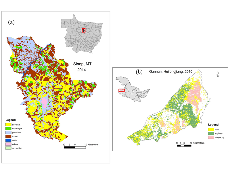
One county, Sinop, Mato Grosso state, Brazil is used to represent the sending system and one county Gannan, Heilongjiang province, China is the representative of the receiving system (Dou et al. 2019). We chose these two counties as study areas because (1) the two counties are similar in size, (2) soybean production is one of the main agricultural activities, (3) we conducted fieldwork in both counties, and (4) their land-use changes are consistent with the overall trends in the major agricultural commodity production regions in the two countries.
Agricultural intensification in the sending system
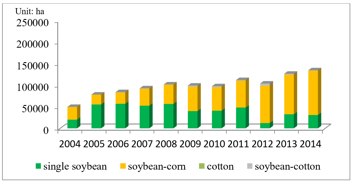
The main land-use phenomenon in Sinop the sending system is agricultural intensification. Multiple studies have found that soybean production in Mato Grosso has shifted from predominantly single cropping systems to majority double cropping systems (Figure 14 in the Appendix). The areas used for single cropping increased from 20,056 hectares in 2004 to 30,885 hectares in 2014, while areas of double cropping have grown almost 3.5 times to 102,810 hectares in 2014 (Kastens et al. 2017). The growth in double cropping is strongly correlated with socio-economic development (e.g., measured by income, literacy, and longevity) and agricultural intensification (Garrett & Rausch 2016; Spera et al. 2014; VanWey et al. 2013).
Crop conversion in the receiving system
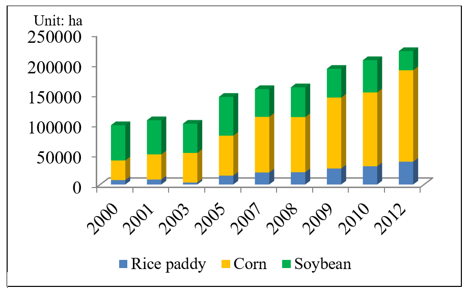
Since the soybean trade boom, farmers in Heilongjiang have converted large areas of soybean land to corn and rice paddies (Figure 15 in the Appendix) (Sun et al. 2018; Sun et al. 2015). The conversion from soybean land to corn land and rice paddies results in increased nitrogen pollution (Sun et al. 2018) and largely alters the landscape, which affects biodiversity and regional water flux. The land-use maps of the two systems are in Figure 1.
Entities, state variables, and scales
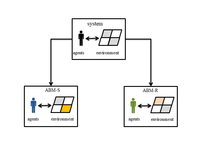
The primary entities in this model are systems, agents and environment. All the entities are hierarchically structured (Figure 2): systems, agents, and environments all have an abstract class in the model with common properties shared between sending and receiving systems. The receiving and sending systems are derived from the abstract module to create an instance of agents and environments for the system with unique properties.
Systems in TeleABM include the overall telecoupled soybean system which has the sending system and receiving system. The land-use changes in the sending and receiving systems are individually represented and interact with each other through the flows of soybean trade, which together constitute the telecoupled soybean system. In each system, there are agents interacting with the environment.
Agents. In both sending and receiving systems, there are farmer agents, trade agents, and government agents (Table 1). In the abstract class, a farmer agent has a list of general properties (e.g., labor, capital, and land property) and a list of common abstract actions (e.g., land-use decision, calculate cost and profit). Farmer agents can be instanced as farmer agent class in the sending system (as a sendingSoybeanAgent class) or farmer agent class in receiving system (as a receivingSoybeanAgent class) based on the system’s initialization. Attributes of agents are drawn from household surveys, information from yearbooks, interviews, and mental models (a mathematical pairwise association that semi quantitatively captures the qualitative knowledge and perceptions of stakeholders (Gray et al. 2015; Mehryar et al. 2018) that were conducted in study areas.
Additionally, there are government agents and trade agents. Government agents decide levels of commodity tariffs, crop subsidies, and trade volumes. International trade agents determine the soybean crop prices based on a partial demand-supply relationship and connect the two systems by flows of soybean commodity and soybean price. Local trade agents disseminate soybean prices and facilitate the trade by collecting soybeans from local farmers.
| Agent Class | Property | Function |
| Farmer Agent | • land property, labor endowments, capital endowments | • read land uses from land-use maps (initialization step) |
| • land cells with current and historical land-use information | • get commodity price | |
| • crop production and profits | • step (execute every year, including abstract function of updating production, updating costs, updating profits, and land-use decisions, updating land uses) | |
| sendingSoybeanAgent | diversifying preferences | land-use decision in the sending system |
| ✓ diversifying preferences | ✓ land-use decision in the sending system | |
| - land-use probability | ||
| - expansion | ||
| receivingSoybeanAgent | ✓ number of family members | ✓ land-use decision in the receiving system |
| ✓ household head gender and age, unhealthy proportion, dependent ratio, knowledge of soybean trade | - rice cultivation | |
| ✓ attitudes towards soybean trade | - soybean and corn cultivation | |
| - allocate crops to suitable cells | ||
| - expansion | ||
| Trade Agent | • capital endowments | • purchase soybeans and pass local prices to local farmer agents |
| • spatial coverage | ||
| sendingTradeAgent | ✓ deliver the international price to local farmer agents | |
| receivingTradeAgent | ✓ deliver the international price to local farmer agents | |
| internationalTradeAgent | ✓ conduct the international soybean trade | |
| Government Agent | • implement top-down policies | |
| sendingGovernmentAgent | ✓ implement environmental policies | ✓ SoyMoratorium scenario (future scenario) |
| receivingGovernmentAgent | tariff imported crops and subsidize domestic crops | ✓ tariff scenario |
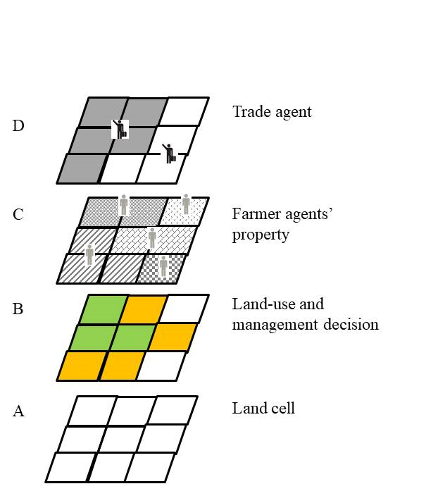
Environment. The environment of TeleABM is based on a grid of cells, typically representing 900 m2 or 0.06625 km2 based on the land-use map resolution (e.g., in the current version, we use 250m \(\times\) 250m land-use maps for the receiving county and 240m \(\times\) 240 m for the sending county, due to data availability). Each cell has defined biophysical properties including empirical data (e.g., temperature, precipitation, elevation, and soil texture) and hypothetical data (e.g., cadastral ownership) (layer A in Figure 3). Cells are assigned to and managed by farmer agents (layer B and C in Figure 3). Crop yields are functions of fertilizer inputs and crop rotation, which are derived from literature and expert opinions from both sites (see Table 4 in the Appendix. Local trade agents interact with farmer agents who are within their spatial coverage (layer C and D in Figure 3), by passing the crop price to these farmer agents and purchasing their crop products.
Process overview and scheduling
The initialization of TeleABM includes three parts: 1) setting the global parameters (e.g., users determine which system(s) to simulate, initialize farmer agents, use static crop price, empirical crop price, or simulated international price), 2) reading land-use and other maps (e.g., suitability map) and external files (e.g., empirical crop prices, subsidy); 3) initializing farmer agents and other agents, including land cells allocation to farmer agents, agents properties setup (e.g. capital, diversifying preference) according to empirical and/or hypothetical data, and farmer agents and trade agents connections.
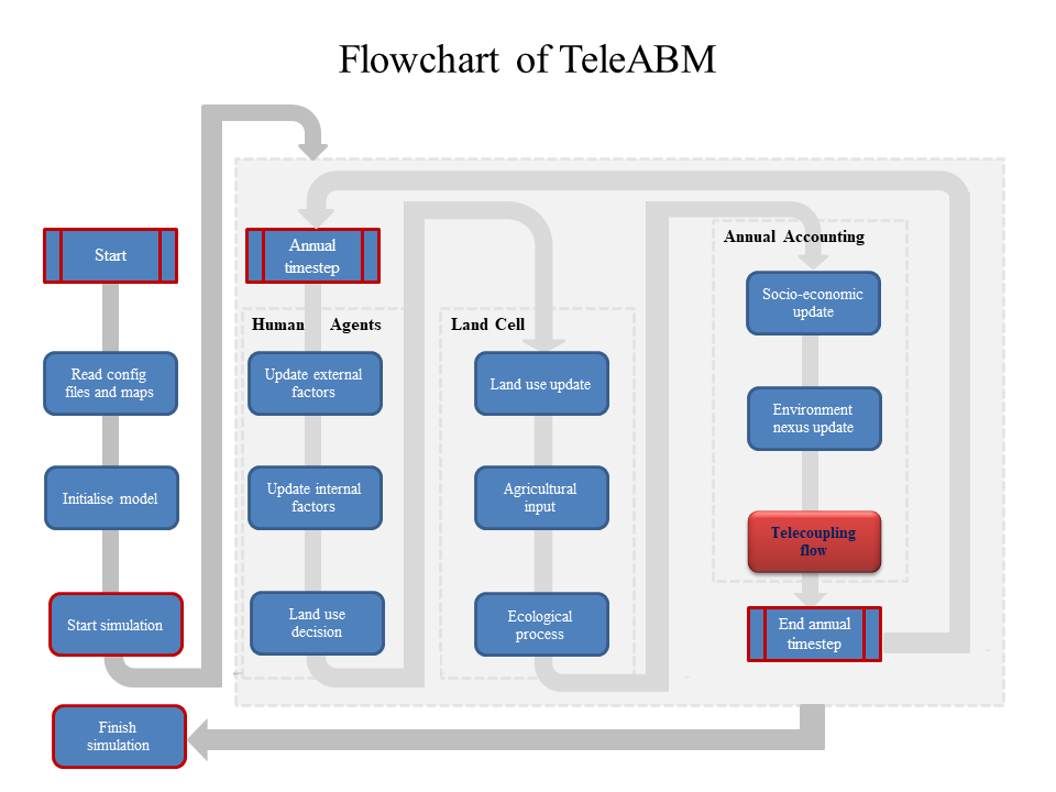
After initialization, TeleABM operates on an annual basis and is divided into major steps of (1) human land-use decisions, (2) land cell changes and (3) annual accounting to update socio-economic and environmental conditions (Figure 4). Once both sending and receiving systems are simulated, telecoupling flows (e.g., the flow of soybean commodity and price) in the annual accounting are triggered, via international trade agents, who facilitate trade and update crop price.
At every time step, the internal agent factors are updated first (e.g. last year’s crop cost and profit), then farmer agents interact with local trade agents to obtain the crop price, which is either exogenous (i.e., if only one system is simulated, price information is given in the price file) or endogenous (i.e. the crop price is updated every year from the international trade agent). Farmer agents in the receiving system allocate their resources to grow soybeans, rice, and corn. Farmer agents in the sending system allocate their resources to grow a single-season of soybeans, a double-season of soybeans and corn, and/or a double-season of soybeans and cotton.
Farmer agents pass the land-use decisions and associated agricultural input (e.g., fertilizer and fuel use) to land cells and update the land use for the current step. Previous land uses are recorded to land cell property. Land cells undergo ecological processes to generate the new crop yield and soil organic matter in response to fertilizer use (Materials Submodels in the Appendix). Sending and receiving systems have separate ecological processes that endogenize local-level environmental variability. However, for simplicity, in the example simulation average crop yield is assigned to each crop to highlight the land-use change aspects.
Once all agents and land cells are updated, the model moves to annual accounting steps during which farmer agents’ profit is calculated and stored, as well as the environmental-impacts (i.e. water usage, fuel input, and crop production). When both sending and receiving systems are initialized, soybean production from the sending system is aggregated through the local trade agents and sent to international trade agent as a flow, so that next year’s crop price is estimated by the international trade agents (Figure 4). When only one system is initialized, the crop price is either a static price from the initialization step or a dynamic price that is read in from a configuration file. After this, the annual time step is finished and the model moves to the next time step.
Design concepts
Here we introduce the theoretical and empirical background, the decision-making representation, and the telecoupling flow. Common concepts of ABMs required by ODD+D are in the Appendix.
Theoretical and empirical background
Telecoupled soybean trade system
TeleABM is designed to test hypotheses that have emerged from the telecoupling framework (Liu et al. 2013). Using the telecoupled soybean system as an example, our model can answer “what-if” questions under alternative scenarios, such as the question in this paper “if China increases its tariff on imported Brazilian soybeans, what land-use outcomes will occur in Brazil as well as China?”. The simulation results from addressing this “what-if” question can be used to evaluate the relationship between the telecoupling process (e.g., trade) and internal processes (e.g., local land use), and to test cascading effect hypothesis (e.g., changes in one land-use system radiate outward to land uses in other systems). Practically, we ask this specific question concerning the current soybean tariff disputes between the United States and China. We hope that although the simulated scenario is between Brazil and China, the land-use consequences can still inspire policy makers in all trading parties.
Individual decision making
We utilize different approaches to construct and validate the land-use change patterns in the two systems due to different fieldwork approaches and data availability. In our case, a household survey was conducted in the receiving system and a mental modelling approach (Özesmi & Özesmi 2004; Van Vliet, Kok, & Veldkamp 2010; Voinov & Bousquet 2010) was used per the project requirement and situation in the study sites (Dou et al. 2019).
Representing decision making in the sending system
Several factors have been indicated to be main drivers of the agricultural expansion and intensification in Mato Grosso, Brazil (Garrett et al. 2013; Garrett & Rausch 2016; Richards et al. 2012), such as topography, climate conditions, and distance to the closest ports. Land-use history is also an important factor in Mato Grosso, because soybean land often replaces land deforested for pasture or previously under pasture. Due to data availability and research interests, we select the previous two-year land-use history (to be consistent with the usual practice in the field (Spera et al. 2014), yield, profit, and elevation, slope, distance to ports, and distance to urban area as explanatory factors (Table 2). Soil property is homogenous in Sinop; therefore we exclude it for this analysis. Using the crop cover maps from 2001 to 2014 that are provided by Kastens et al. (2017), we apply a multi-nomial logistic regression to calculate the probability of agricultural land use at year \(t\).
| $$\text{prob}(lc_{i,t}) = f(lc_{t-1}, lc_{t-2}, C_{i, t-1}, P_{i, t-1}, S_i, \textit{elevation}, \textit{slope}, \textit{distance})$$ | (1) |
| Unit (real/ha) | single-soybean gross return | soybean-corn gross return | soybean-cotton gross return | single-soybean cost | soybean-corn cost | soybean-cotton cost |
| year 2005 | 1833 | 3125 | 12148 | 1975 | 4410 | 8140 |
| year 2010 | 2475 | 4285 | 11628 | 1611 | 3531 | 6529 |
| Unit (meters) | distance to urban | distance to roads | elevation | Slope | ||
| mean value | 17830 | 8173 | 364.6 | 0.982 |
In addition to land-use probability, farmers’ decision making is incorporated. Two factors (i.e., capital capacity and preferences for diversification) are identified as significant by soybean producers that we interviewed during fieldwork. In the model, even if the probability suggests double cropping, farmer agents would only be able to implement single cropping without enough capital endowments. The other property, “pro-diversifying”, is extracted from the fieldwork conducted by our team in the summers of 2016 and 2017. The preliminary analysis suggests that farmers in Brazil have different risk-taking attitudes. In current simulation, farmer agents are split evenly between the two risk-taking attitudes (50% simulated agents as “pro-diversifying” and 50% not) as a hypothetical distribution to even out the effects of this attitude, which will be explored in future work. The pro-diversifying farmer agents have a higher probability of choosing double cropping over single cropping when all other factors hold the same.
Representing decision making in the receiving system
The land-use changes in the receiving system mostly appear on small-scale farms which are operated by household labor. It is necessary to first establish crop suitability maps because rice paddy needs special topography and water condition. We then analyze land-use changes based on the extensive household survey conducted in the summer of 2017 to quantify the land-use decisions at the household level.
Crop suitability
First, empirical data on soil type (Institute of Soil Science-Chinese Academy of Science 2019; Liu et al. 2006), accumulated temperature (\(\geq\) 10\(^{\circ}\)C) (Li et al. 2014; National Meteorological Information Center 2019), distance to water and distance to roads (calculated using ArcMap) are collected. Then, the multinomial logistic regression is used to calculate the probability based on the 2005 and 2010 spatial distribution of the three crops classified from remote sensing images and these land-use factors. This probability of crop presence is used as a proxy for suitability which is a common practice in land use and ecological modelling (Chen et al. 2010; Magliocca, Brown, & Ellis 2013; Walsh et al. 2013). Last, the higher probability among the two time points is selected as the crop suitability, in case suitability has changed due to crop conversion (Figure 5).
The choice of which crop to grow is a complex decision, and it is particularly true among smallholder farming households (An 2012; An et al. 2005; Huber et al. 2018). The representation of farmers’ land-use decisions crucially depends on the purpose of the study and the attributes of the system. There are many decision-making mechanisms and rules used in modelling farmer agents’ crop choice, among which the statistical regression model is often used to describe the relationship between land-use patterns and empirical farmers’ attributes (e.g., LUDAS, see Le et al. 2008; Chen et al. 2014). Many factors have been noted crucial to the crop/land-use choices by smallholders, such as the dependent ratio that measures the number of dependants to farm workers and reflects the number of mouths each worker feeds (Chayanov 1966; Le 2005), the gender ratio that measures the number of adult males over the total number of family members (Walsh et al. 1999), the education level of the household heads and family members (An et al. 2002; Dou et al. 2017), and the size of off-farm income (Dou et al. 2017; Yang et al. 2018).

| variable abbr. | HHage | Hfm | Rdep | Rg | Edu | Ns | Nm | Ruh |
| variable names | Household head age | number of family members | dependent ratio | gender ratio | average school years | number off- farm salary | number of big machines | unhealthy proportion |
| mean value | 44.8 | 3.672 | 0.2184 | 0.1346 | 9.721 | 0.4647 | 2.908 | 0.05615 |
| variable abbr. | Ad | Ap | FCsoybean | FCcorn | FCrice | GIsoybean | GIcorn | GIrice |
| variable names | rain-fed area (ha) | paddy area (ha) | soybean fertilizer cost (yuan/ha) | corn fertilizer cost (yuan/ha) | rice fertilizer cost (yuan/ha) | soybean gross income (yuan/ha) | corn gross income (yuan/ha) | rice gross income (yuan/ha) |
| mean value | 3.371 | 2.198 | 347.2 | 870.1 | 1054.2 | 2847 | 4595 | 4599 |
| variable abbr. | HHg | K | HHedu | DEL | ||||
| variable names | household head gender | whether know soybean import | education of household head | |||||
| head count | male 400; female 11 | No: 146; Yes: 265 | illiterate: 2 | elementary school: 56 | middle school: 261 | high school: 79 | college: 13 | |
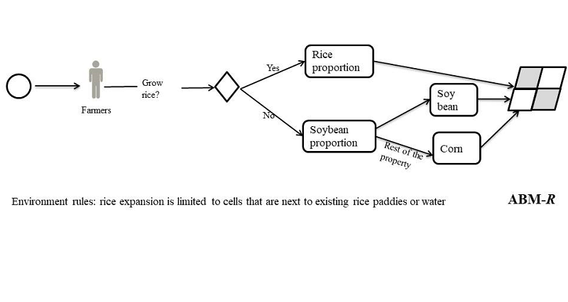
In the receiving system of TeleABM, several tiers of statistical relationships are used to represent the land-use behaviors of these farmer agents (Figure 6). If agents engage in agriculture in a given year t, they 1) first decide the proportion of rice to cultivate on the whole property, 2) decide the proportion of soybeans and corn to cultivate, and then 3) allocate cells that are suitable for cultivating these crops. Data on farmer agents’ attributes were collected during a household survey in the year 2017 (total count: 411, Table 3), which were tested for collinearities and used for calculating the statistical relationships.
Rice cultivation proportion among rice-farmers
| $$\text{prop}(\textit{Rice}_t = f(HH_{\textit{age}}, H_{fm}, R_{\textit{dep}}, R_g, R_{uh}, \textit{Edu}, N_s, N_m, A_d, A_p, FC_{i,t}, GI_{i,t}, HH_g, K, HH_{\textit{edu}}$$ | (2) |
The receiving land-use module calculates the proportion of rice in a receiving farmer agent at the current year t using regression analysis. Only the rice cost and profit are used to calculate this proportion (\(FC_{i,t}\) and \(GI_{i,t}\) are rice cost and gross income at the year \(t\)). These variables (Table 3) are initialized following the empirical distribution using the Monte Carlo approach. The proportion of corn and soybeans is assigned using the distribution of the two crops collected from the survey.
Soybean cultivation proportion in non-rice farmers
For farmer agents that do not grow rice, the proportion of soybeans is calculated using the following regression equation, and the corn proportion complements to 100%. This is because based on soybean and corn suitability, soybeans and corn are likely interchangeable. The \(FC_{i,t}\) and \(GI_{i,t}\) here are soybean cost and gross income at the year \(t\).
| $$\text{prob}(\textit{Soybean})_t=f(HH_{\textit{age}}, H_{fm}, R_{\textit{dep}}, R_g, R_{uh}, \textit{Edu}, N_s, N_m, A_d, A_p, FC_{i,t}, GI_{i,t}, HH_g, K, HH_{\textit{edu}})$$ | (3) |
Allocate cells
For a receiving farmer agent \(i\) that owns \(N\) number of land cells, it first sorts its \(N\) land cells by rice suitability and then allocates \(N_r=N\ast \text{prop}(\textit{rice})_t\) to cultivate rice for year \(t\). However, these cells have to be either rice paddy, or next to a rice paddy or water. Otherwise these cells are assigned to grow soybean or corn. The rest of the cells are sorted by soybean and corn suitability and allocated to soybean and corn cells respectively.
Property expansion
A receiving farmer agent can also reclaim non-agricultural cells as agricultural cells. We assume that every year the agent reclaims some new areas as agricultural land (i.e., follows a \(u=\)0.2, \(\delta=\)0.05 Gaussian distribution for a hypothetical constant-paced expansion). The reclaimed cells are assigned to the highest profitable crop.
Telecoupling features
TeleABM can simulate solely the sending system and its land-use changes, or the receiving system and its land-use changes, or both systems and their telecoupled interactions during one simulation. In this section, we describe how the telecoupling feedbacks are represented in this model.
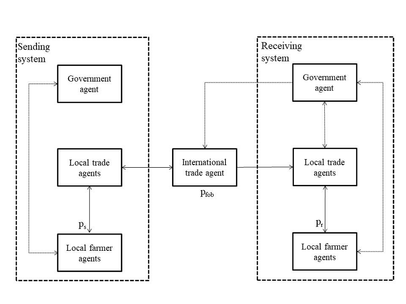
Model structure of telecoupling feedbacks
In each system, there are one government agent, local trade agents, and farmer agents. The two systems are connected through an international trade agent (Figure 7). In the sending system, farmer agents make land-use decisions based on a local soybean price (\(p_s\)). Local trade agents purchase soybeans from local farmer agents, which are aggregated to the international trade agent. The total traded volume of soybeans from the sending system affects international soybean price (\(p_{\textit{fob}}\)), which is passed to trade agents in the receiving system. This price is then distributed to local farmer agents (\(p_r\)). The government agent in the receiving system sets up a subsidy based on the aggregated soybean production in the receiving system, which aims to meet a certain quantity of domestic production.
Telecoupling flows in the model
Many factors affect international soybean trade and thus change the soybean prices. Such factors include tariff disputes, transportation system improvements, favorable climate conditions or climatic hazards, and exchange rate fluctuations. It is unrealistic to include all potential factors and relationships in one model. We simplify the model by focusing on the land-use changes driven by the soybean supply and demand dynamics only. Several assumptions are applied to this international trade simplification: 1) the supply and demand relationship between Brazil and China determines their traded soybean price; 2) the two counties used as model examples represent the average land use and trade conditions in the two countries. In TeleABM, we use several relationships (e.g., elasticity) between soybean price and the supply-demand quantity obtained from literature to represent the dynamics of telecoupling flows between the sending and receiving systems.
Sending system affects international soybean prices
We assume the supply of soybean production affects the international soybean price (\(p_{\it{fob}}\)), and we use an export demand elasticity to measure this dynamic. The export demand elasticity measures the percentage change in exports associated with the 1% change in the price of the exporting country \(p_{\it{fob}}\) (Reimer2012). We assume this export demand elasticity is fixed in the short run, and pfob is only affected by the supply changes resulted from mixed production changes (\(Q^t - Q^{t - 1}\)) in the sending system that are caused by climate, land-use change, and other factors. We apply the empirical point elasticity (-0.9) obtained from (2012) and calculate the price at year \(t\) given export change and price at year \(t-1\).
| $$p_{\textit{fob}}^t=p_{\textit{fob}}^{t-1} + p_{\textit{fob}}^{t-1} \cdot \frac{EQ^t - EQ^{t-1}}{\epsilon_{ep}\cdot EQ^{t-1}}$$ | (4) |
| $$EQ^t=Q^t$$ | (5) |
International soybean price conversion to local prices
To local prices in the sending systems: Local prices in the sending system could also be impacted by its external factors, such as the global fuel price (\(p_{\textit{fuel}}\) US\) per gallon), the proportion of Brazilian soybean production over the global soybean production (\(R_B\)), and the proportion of Chinese soybean import over the global soybean production (\(R_C\)), 2009 “zero-deforestation” supply-chain initiative (Gibbs et al. 2016) ((ZD dummy (0\(=\)no, 1\(=\)yes)). Global soybean production reflects the climate effect and the global economy. Fuel price has proved a significant factor in global agricultural trade. The proportion of soybean import over global soybean production reflects the overall economy and demand of China. We thus convert international soybean prices calculated above to Brazil’s local soybean prices using the following calibrated regression:
| $$p^t_s=f(p^t_{\textit{fob}}, p_{\textit{fuel}}, R_B, R_c, ZD)$$ | (6) |
To the local prices in the receiving system: We employ a price transmission elasticity function (Reimer et al. 2012) to convert international soybean prices (\(p_{\textit{fob}}^t\)) to China's local soybean prices (\(p_r^t\)), given local prices in the last year (\(p_r^{t-1}\)), the current international soybean prices, the trend (\textit{year}), together with several other exogenous factors used above (i.e., \(p_{\textit{fuel}}\), \(R_C\)), as well as local prices of corn and rice at current year \(t\) (\(p_{\textit{corn}}^t\) and \(p_{\textit{rice}}^t\)). Local prices of corn and rice in the current year represent government policy on stockpiling and incentives. This price transmission function from international soybean prices to China's local prices can be specified as:
| $$\ln p_r^t=\beta_0+\beta_1\ln p_r^{t-1}+\beta_2\ln p_{\textit{fob}}^t+\beta_3 \textit{TREND}+\beta_4 p_{\textit{fuel}}+\beta_5 R_C + \beta_6 p_{\textit{corn}}^t + \beta_7 p_{\textit{rice}}^t$$ | (7) |
High-tariff scenario: elasticity of China’s soybean demands
In a high-tariff scenario, we try to investigate the soybean import volume changes due to the tariff-driven price increase. A tariff increase in China that imposed to Brazilian soybeans will boost China’s received soybean prices from Brazil (\(p_{\it{fob}}^{t-1}\)). For this purpose only, we apply a bilateral import demand elasticity \(\epsilon_{ep}\) for China with respect to Brazilian soybeans. It means that a price increase in \(p_{\it{fob}}\) will lower China’s soybean imports and thus impact Brazilian soybean exports and production. We followed the method from Reimer et al. (2012) and calculated the import demand elasticity of China with respect to Brazilian soybeans using the data over the years of 2009-2015 (Hjorth & Wilensky 2019; Bank 2019; UN Comtrade 2019). The import demand elasticity measures the percentage changes of import quantity \(\Delta IQ\) with respect to one percent changes in Brazilian soybean price \(\delta p\). We use data after 2009 to avoid the potential noise of 2007 and 2008 when there was a world food price and economic crisis. The calculated elasticity \(\epsilon_{ip}\) is approximately -0.29, meaning one percentage increase of soybean import price will reduce China's import by 0.29 percent.
| $$\Delta IQ = \frac{\epsilon_{ep}\cdot \Delta p\cdot IQ^{t-1}}{p_{\textit{fob}}^{t-1}}$$ | (8) |
Validation
The validation of TeleABM requires two sequential processes: validation of the sending/receiving system independently, and then the validation of the flow between them. Due to different data availability and decision-making representation in the two systems, the validation methods are also different.
Validation of decision making in the sending system
Two years’ (t = 2007 and t = 2012) land-use data are selected to validate the regression results using the receiver operating characteristics (ROC curve, presented in Figure 8). ROC is a commonly used measure of goodness-of-fit in classification problems (Chen et al. 2014; Sun & Müller 2013). A ROC curve is derived by plotting the rate of true positives versus the rate of false positives. We select years 2007 and 2012 because one is in the earlier period and the other is at the later period over the simulated 10 years (2005-2015). The areas under the ROC curve for all three crops in both years are larger than 0.8.

Validation of the receiving system
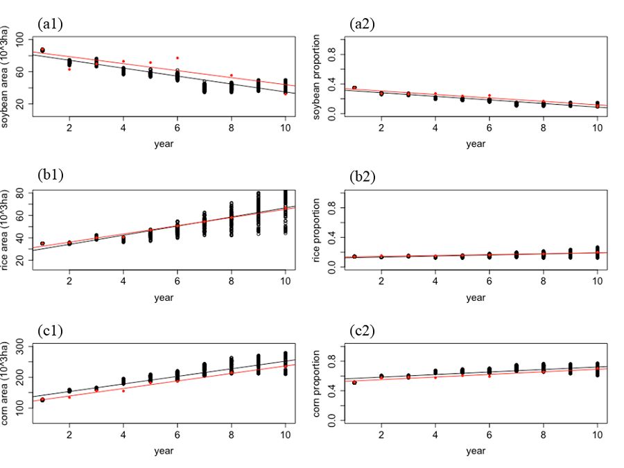
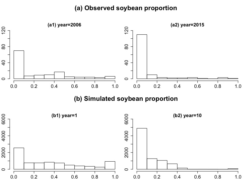
In the receiving system, pattern-oriented modelling approach (POM) is used to calibrate and validate the simulation results. The POM is a strategy to construct and validate the model with multiple observed patterns at different scales and scopes of the modeled complex system (Castella & Verburg 2007; Grimm & Railsback 2012; Grimm et al. 2005). If a model can reproduce multiple patterns observed in real systems, we think it is less likely to falsify the model design than the ones that reproduce only one or no pattern. We compare patterns of agricultural land-use change at two levels: the crop planted areas and proportion at the county level (the aggregated area and aggregated proportion) (Figure 9) and the soybean proportion at the household level (Figure 10).
At the aggregated level, the slope coefficients between time and the simulated crop area are compared with the slope coefficients between time and the empirical crop area by t-test (e.g., we compute the t-test statistics by dividing the difference between the two slopes over the residual variance see Wuensch 2018). The results are not significant for all three crops, which indicate that the receiving system of TeleABM can reproduce the changing pattern of planted areas and the proportion of the three crops.
At the household level, the soybean proportion of each agent (i.e., simulated soybean area over the total household agricultural area) at the beginning of the simulation (year 1) and at the end of the simulation (year 10) are recorded and compared with the reported soybean proportion from the household survey. The pattern of individual soybean proportion is that more farmers abandoned soybean cultivation or largely reduced the soybean proportion. Although the simulated soybean proportion distribution is not statistically identical to the observed distribution (using Kolmogorov-Smirnov test), we believe that the model can represent the pattern of farmers reducing and/or abandoning soybean production in the receiving system. The difference in distribution may be due to the hypothetical initialization of properties.
Validation of the telecoupling feature
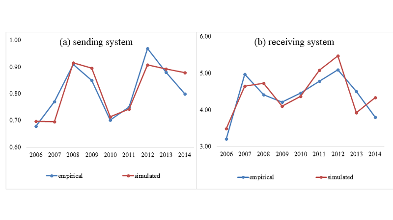
The soybean price in the sending system is affected by the production change in the sending system and this price will affect the local soybean price in the receiving system along with other factors such as fuel price. Therefore, the simulated soybean prices in both systems are compared with empirical data, and t-tests show no significant difference which indicates the telecoupling module of our model can reproduce the empirical price dynamics (Figure 11).
A Sample Simulation
To show how the results can be used to understand telecoupling features, we include a simple sample simulation. The sample simulation has two settings: (A) Baseline scenario - no tariff, and (B) High-tariff scenario - 25% tariff. In scenario (A), a business-as-usual international trade is assumed. This means that the international soybean price is determined only by the change of soybean production from the sending system, as well as the exogenous global factors such as average global fuel price. In scenario (B), a 25% tariff is charged on the soybean production from the sending system to the receiving system starting from simulated year 5. The soybean price is then affected by both the import demand elasticity and export demand elasticity. All the other settings are the same. To eliminate randomness in the initialization and modelling process, 20 replicates are simulated for 10 years each.
Less agricultural intensification in the sending system at the tariff scenario
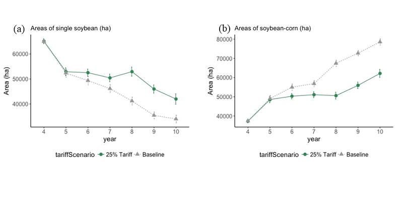
The land-use changes in the sending system under the tariff scenario are compared to the baseline scenario (no tariff) (Figure 12). Both scenarios indicate that the double-soybean planted area (soybean-corn) increases while single soybean cultivation decreases. However, when the tariff charge starts at year 5, fewer cells are converted to soybean-corn each year, and more cells are converted to single soybean compared to the business-as-usual scenario. This suggests that the tariff slows down the intensification on Brazilian soybean farms, because farmers may not be able to prepare for a second growing season since they get less profit from the soybean trade.
Cascading effect on the land-use changes in the receiving system
A cascading effect (i.e., chain events caused by the trade of one crop affecting other systems and components (Silva et al. 2017) is also observed in this sample simulation. The tariff not only affects the land uses in the sending system but also affects land-use changes in the receiving system (Figure 13). The tariff drives the Brazilian soybean price and production down due to less demand from China which, in turn, affects the international soybean price. In the receiving system, because soybean imports are lower than domestic demand, the government agent provides a subsidy to local farmers for added soybeans to their crop cultivation (5,000 yuan/ha). This changes farmers’ preference from corn to soybeans and slows crop conversion from soybeans to corn in the receiving system. The differences between the baseline scenario and the tariff scenario in the receiving system start from year 6, which is one year later than the sending system (year 5) as a cascading effect.

Discussion
Different approaches used for receiving and sending system land-use simulation
To the best of our knowledge, there is no model in current ABM applications that represent two distant land systems in one model. As mentioned above, the individual systems in our model (i.e., sending and receiving systems) vary in agent attributes, behaviors, interactions, and market structure. One of the challenges of building telecoupled ABMs is to represent the land use and decision making of two very different land systems. Moreover, the available datasets for the two systems are most likely not interoperable. Fieldwork outcomes from the two systems are also very different: a quantitative database that details hundreds and thousands small farming households’ characteristics and land-use information in the receiving system, and a mixed qualitative and quantitative dataset that describes dozens of large soybean producers in the sending system. The key is to identify the common features and variations in both systems and minimize the modelling workload. This is discussed in detail in another article that focuses on the design philosophy of TeleABM (Dou et al. 2019).
Aggregated errors from local simulation to telecoupling simulation
Another major challenge of TeleABM is validation, similar to many other modeling efforts (Van Vliet et al. 2016) . The validation of ABMs can use either the structure or the model outcome (Evans 2012; Millington, Demeritt, & Romero-Calcerrada 2011). For TeleABM, we need to validate both the individual system as well as the flows between the two systems. Therefore, in total three validations are conducted for TeleABM. Validation methods for the sending and receiving systems differ and are based on data availability. For the sending system, the land use is validated by using a ROC curve while in the receiving system, the land-use simulation results are validated by the pattern-oriented approach. The flow between the receiving and sending systems is compared to the simulated soybean price with the historical local soybean prices. Based on insights gained during the validation process, we recommend the integration of many datasets from multiple coupled human-natural systems into a common, interoperable database following the telecoupling framework. This will eliminate errors for calibration and validation.
The flow between the two systems is represented by the supply and demand function and calibrated with several other global factors (e.g., average fuel price). For validation, we use the simulated soybean supply from the sending system to feed the international soybean trade agent, which is different from the empirical soybean supply. Although this difference (between empirical soybean supply and simulated soybean supply) is within the acceptable range, it may be passed from the international soybean trade agent to local soybean trade agents in China, creating a larger deviation of soybean price in the receiving system from the empirical soybean price.
Alternative modelling structures
One of the shortcomings of ABMs is the YAAWN syndrome (Yet Another Agent-Based Model … Whatever… Nevermind…), which addresses that many ABMs in land science are case-specific (O’Sullivan et al. 2015). There have been attempts to easily apply ABMs from one place to other places, such as proposing generalized modelling frameworks including MP-MAS (Marohn et al. 2013; Schreinemachers & Berger 2011) and the CRAFTY framework (Arneth, Brown, & Rounsevell 2014; Blanco et al. 2017; Murray-Rust et al. 2014), or using inter-model comparisons to identify the common attributes and functions (Huber et al. 2018; Parker et al. 2009).
The presented model is constructed from empirical data and common variables from land system science, rather than following CRAFTY or a similar modelling framework. This is because these frameworks are often accumulated from European land-use changes and modelling. It may underrepresent certain important features if applying such frameworks in agricultural frontier (Brazil) or in small farming households (China), or require rich datasets to calibrate. As new research pointed out, in urban studies the field is dominated by global north researchers which underrepresent urgent issues in the global south (Nagendra et al. 2018). Our decision-making processes in the sending and receiving systems are both based on widely used statistical methods (e.g., logistic regression); hence it can be easily adopted by other cases with similar properties.
Some scholars have suggested to the first author to use individual ABMs and then connect the simulation results in a different program (e.g., system dynamics models or computable general equilibrium model) instead of the current format as simulating multiple systems in one model. This indeed is the approach that another project adopted for studying the telecoupling land-use changes in Brazil (Millington et al. 2017). However, we argue that the focus of this other telecoupling project is solely on the local land-use changes in Brazil in the telecoupled soybean system. What we care most about and what insights our model can offer is the causes and effects of local land-use changes on the other land systems. Moreover, if we externalize the feedbacks in another program, the validation might be an additional challenge since it is difficult to adjust the chain of changes in local land systems caused by the change from the flow.
Future directions and policy implications
The design, development and implementation of the first ABM that represents land-use changes in two systems distantly connected through trade flows opens new research avenues for many issues in different research fields, such as the sustainable governance in land system science and environmental impact assessment of international trade. In the present study, we simplify international trade dynamics by only modeling flows between the sending and receiving systems. Future work could expand upon this by simulating flows between multiple senders and receivers as well as flows to spillover systems. For example, TeleABM could be expanded to include land-use change in the United States, the second largest soybean producer and exporter. Producers in the U.S. are affected by trade dynamics between Brazil and China and vice versa. Spillover systems are one of the most elusive and underrepresented components in current telecoupling studies (Jianguo Liu, Dou, et al., 2018). For example, TeleABM could be improved by including some emerging soybean producing regions (e.g., Argentina, Uruguay).
TeleABM can play multiple roles within land system science and can be used to derive policy implications. First, TeleABM addresses the omission of distant land-use actors and processes in current land-use modeling practise (Verburg et al. 2019). The underlying mechanisms of certain land-use demand that are generated from outside of the modeled area can be explicitly represented in one model. Second, we can employ the model to simulate potential policies and technology changes in one system and evaluate the responses in its telecoupled partners. For example, in the high-tariff scenario, potential subsides from Brazilian government to local soybean farmers could reshape land uses in China. In the future, improvements in domestic transportation and port access will influence Brazilian farmers’ production decisions and thus potentially affect China’s land-use changes. Meanwhile, China’s efforts to protect its natural land cover (Liu et al. 2018), such as the Grain-to-Green Program (Liu et al. 2008), could reduce China’s crop production, incentivize imports from its trading partners, and impact land uses in the exporting country. Lastly, as a tool to analyze distantly coupled human-natural systems, TeleABM can enable researchers and policy-makers evaluate potential trends and policies, such as land consolidation and crop diversity, to achieve food security and sustainable development in the overall food production system including both importing and exporting regions.
Conclusion
In this study, we develop TeleABM, a novel telecoupled agent-based model using a hierarchical modelling structure and the telecoupling framework. The validated model is used for a sample simulation of a high-tariff scenario on international soybean trade and the effects on land-use changes in both sending and receiving systems were demonstrated. TeleABM is useful in three major aspects. First, it fills a gap in current land systems science. Besides assessing the one-way land-use changes under external forces, it demonstrates land-use feedbacks between distant land systems. Second, it is a valuable research tool for testing telecoupling hypotheses and quantifying telecoupling relationships across distant land systems. Last, the experiences and lessons learned through its construction can be used to advance the methodology of agent-based modelling, since no ABM has simulated more than one land system simultaneously.
Acknowledgements
This work is supported in part by the US National Science Foundation (1518518), Michigan State University, and Michigan AgBioResearch. We thank Sue Nichols for her constructive comments and edits, and many colleagues and friends including Dr. Qingxu Huang, Dr. James Millington, and Dr. Paul McCord for their helpful critiques and insights.Model Documentation
The model was implemented in RePast Simphony 2.4 (https://repast.github.io/download.html). The code is available at: https://www.comses.net/codebases/c7e925e0-a228-4e56-81e9-07455f453497/releases/1.0.1/.Appendix
| Year | Sending system | Year | Receiving system | |
| Sinop, Mato Grosso, Brazil | Gannan, Heilongjiang, China | |||
| area (km2) | 3,194 | 4,792 | ||
| population | 2017 | 135,874 | 2012 | 390,000 |
| soybean planted area (km2) | 2017 | 1,437 | 2012 | 318 |
| soybean production (tons) | 2016 | 403,200 | 2012 | 56,335 |
| soybean yield (kg/ha) | 2016 | 3300 | 2015 | 2007 |
Common ABM concepts represented in the model
The feedback between distant places is the primary feature of TeleABM. To follow the ODD+D protocol, we still document the following properties even though some concepts are not used in this paper.
Emergence
Farmer agents’ land-use behaviors are expected to vary when their characteristics are initialized differently, the crop subsidy changes, and by the trading/climate scenarios. The expansion of rice paddy in the receiving is expected to emerge as well as the expansion of soybean-corn in the sending system.
Adaptation
Farmer agents do not change their decision-making rules. However, they adjust their land-use behaviors according to the crop price, profit, labor, previous land use, and other factors.
Objectives
Farmer agents in both systems try to maximize the suitability of the land cells in their property.
Learning
Farmer agents in the two systems update the crop profit every year. They also learn from their neighbors about the crop profit and use it to decide next year’s land-use decision, if they do not grow the crop at current year.
Fitness
No survival fitness is included in the model.
Prediction
Farmer agents are not able to predict accurate crop price for next time step.
Sensing
Farmer agents can sense the crop profit of neighbour agents if they themselves do not grow this crop.
Interaction
Direct interactions occur between farmer agents and local trade agents. Direct interactions also happen between neighbour agents from observing each other and affecting the landscape (e.g., only when a neighbouring cell is rice paddy one can change it to rice paddy). Indirect interactions occur between farmer agents in the sending and receiving systems through international trade agents. Farmer agents also interact with the environment through land-use decisions and management.
Stochasticity
Farmer agents have individual variation in attributes and decision-making parameters, which are drawn from survey data and set as statistical distribution. Furthermore, noises are added to crop management (e.g. a random number is added to fertilizer input and yield) and crop price (e.g. the crop price sensed by farmer agents have a small random value).
Collectives
The crop production from individual farmer agents is aggregated at the end of each time step, and enters the international trade agent. The crop price generated by the international trade agent later affects the individual land-use changes in both systems. Government agent also implements certain policies by reviewing the aggregated land-use results.
Heterogeneity
Heterogeneity is represented by farmer agents’ properties, such as farm size and education. It is also determined by varying certain decision-making features, such as pro-diversifying in the sending system.
Observation
At each time step, land uses are recorded at each farmer agent level, as well as their capital and environmental usage (e.g. fertilizer use, yield, water usage).
Path dependence
Land-use decision of cell i at step t is affected by the land use of this cell at previous steps. The influence comes from (1) soybean farmer agent’s knowledge of different crops, (2) land-use history that affects current crop choice and yield, (3) neighbours’ land-use conversions from and to rice paddy can affect the possibility of agent’s rice paddy decisions.
Details
Initialization
The initialization includes three parts:
Users set up global parameters: users determine which system(s) to run simulation on, the scenario of crop prices, and number of initial farmer agents and vision.
- static crop price: the model reads crop price written by users at the panel, and will stay the same over the simulation time steps
- dynamic crop price: the model reads files that include crop price at every year
- telecoupling feature: the model has sending and receiving systems, and exchange price information during simulation.
The model reads configure files and maps to initialize land cells:
- crop land-use maps from remote sensing data
- empirical crop suitability map
- empirical or hypothetical soil map
The model initializes agents and their characteristics:
- initialize parameters for each system, such as the range of production cost
- several attributes of agents (e.g. capital, gender ratio, education) are initialized based on weighted or normal distribution drawn on statistical distribution from survey data and other sources.
Input data
TeleABM uses three types of input data, which also corresponds to three initialization steps.
| Input file | Function |
| Parameter setting | sending system representation receiving system representation number of initial farmer agents in sending system number of initial farmer agents in receiving system price of crops (soybean, corn, rice, cotton): if >0, static price, if<0, use dynamic price or use telecoupling price |
| Bio-physical data | land-use maps (classified MODIS images (2005 and 2010) and Landsat images (2000, 2006, 2011, 2016, as a verification source) of Gannan, Heilongjiang, and PRODES data (2004-2014) of Sinop, MT) temperature and precipitation map (empirical data, such as maps of annual accumulated temperature above 10°C and maps of precipitation of Heilongjiang) maps of soil types maps of elevation and slope |
| Socio-economic scenario | text files contain annual price of crops different settings of tariff maps of distance to urban and roads |
Submodels
Ecological model. In this model (LandCell class in the receiving system), yield of crops (converted to land cell spatial unit from per ha) is a function of fertilizer, precipitation, and temperature, based on relationships found in literature. However, in this version, we do not include the crop yield response to fertilizer use in the receiving system. Crop yield is a constant value using the survey average (i.e., soybean 2,008 kg/ha, corn yield 9,597 kg/ha, and rice 8,112 kg/ha). In the sending system, the parameterization of each crop yield is given based on experts’ opinion (Table 6). For instance, if a cell is used as soybean-corn, the soybean yield is 3,007.2*90% kg/ha and the corn yield is 4,120*100% kg/ha.
| crop | average yield (kg/ha) | land use | parameter (%) |
| soybean | 3007.2 | single soybean soybean-corn soybean-cotton | 105 95 95 |
| corn | 4120.0 | soybean-corn | 100 |
| cotton | 3346.2 | single cotton soybean-cotton | 105 95 |
References
AN, L. (2012). Modeling human decisions in coupled human and natural systems: Review of agent-based models. Ecological Modelling, 229, 25–36. [doi:10.1016/j.ecolmodel.2011.07.010]
AN, L., Linderman, M., Qi, J., Shortridge, A., & Liu, J. (2005). Exploring complexity in a human–environment system: an agent-based spatial model for multidisciplinary and multiscale integration. Annals of the Association of American Geographers, 95(1), 54–79. [doi:10.1111/j.1467-8306.2005.00450.x]
AN, L., Lupi, F., Liu, J., Linderman, M., & Huang, J. (2002). Modeling the choice to switch from fuelwood to electricity: implications for giant panda habitat conservation. Ecological Economics, 42, 445–457. [doi:10.1016/s0921-8009(02)00126-x]
ANDRIAMIHAJA, O. R., Metz, F., Zaehringer, J. G., Fischer, M., & Messerli, P. (2019). Land Competition under Telecoupling : Distant Actors ’ Environmental versus Economic Claims on Land in North-Eastern Madagascar. Sustainability, 11(3), 1–23. [doi:10.3390/su11030851]
ARNETH, A., Brown, C., & Rounsevell, M. D. A. (2014). Global models of human decision-making for land-based mitigation and adaptation assessment. Nature Climate Change, 4(7), 550–557. [doi:10.1038/nclimate2250]
BALDOS, U. L. C., & Hertel, T. W. (2015). The role of international trade in managing food security risks from climate change. Food Security, 7, 275–290. [doi:10.1007/s12571-015-0435-z]
BANK,W. (2019). World Development Indicators[WWWDocument]. Retrieved from: http://vu-nl.idm.oclc.org/login?url=https://datacatalog.worldbank.org/dataset/world-development-indicators
BARONA, E., Ramankutty, N., Hyman, G., & Coomes, O. T. (2010). The role of pasture and soybean in deforestation of the Brazilian Amazon. Environmental Research Letters, 5(2), 024002. [doi:10.1088/1748-9326/5/2/024002]
BLANCO, V., Brown, C., Holzhauer, S., Vulturius, G., & Rounsevell, M. D. A. (2017). The importance of socio-ecological system dynamics in understanding adaptation to global change in the forestry sector. Journal of Environmental Management, 196, 36–47. [doi:10.1016/j.jenvman.2017.02.066]
BUTLER, R. a., Koh, L. P., & Ghazoul, J. (2009). REDD in the red: palm oil could undermine carbon payment schemes. Conservation Letters, 2(2), 67–73. [doi:10.1111/j.1755-263x.2009.00447.x]
CASTELLA, J.-C., & Verburg, P. H. (2007). Combination of process-oriented and pattern-oriented models of land-use change in a mountain area of Vietnam. Ecological Modelling, 202(3–4), 410–420. [doi:10.1016/j.ecolmodel.2006.11.011]
CHAYANOV, A. V. (1966). The theory of Peasant Economy (1st ed.). Homewood, IL: Irwin,
CHEN, X., Vina, A., Shortridge, A., An, L., & Liu, J. (2014). Assessing the effectiveness of payments for ecosystem services: An agent-based modeling approach. Ecology and Society, 19(1), 7. [doi:10.5751/es-05578-190107]
CHEN, Y., Li, X., Liu, X., & Liu, Y. (2010). An agent-based model for optimal land allocation (AgentLA) with a contiguity constraint. International Journal of Geographical Information Science, 24(8), 1269–1288. [doi:10.1080/13658810903401024]
CHEN, Y., Li, X., Liu, X., Zhang, Y., & Huang, M. (2019). Tele-connecting China ’ s future urban growth to impacts on ecosystem services under the shared socioeconomic pathways. Science of the Total Environment, 652, 765–779. [doi:10.1016/j.scitotenv.2018.10.283]
D’ODORICO, P., Carr, J. A., Laio, F., Ridolfi, L. & Vandoni, S. (2014). Feeding humanity through global food trade. Earth’s Future, 2(9), 458–469.
DOU, Y., Silva, R. F. B. d., Yang, H., & Liu, J. (2018). Spillover effect offsets the conservation effort in the Amazon. Journal of Geographical Sciences, 28(11), 1715–1732. [doi:10.1007/s11442-018-1539-0]
DOU, Y., Deadman, P., Robinson, D., Almeida, O., Rivero, S., Vogt, N., & Pinedo-Vasquez, M. (2017). Impacts of Cash Transfer Programs on Rural Livelihoods: a Case Study in the Brazilian Amazon Estuary. Human Ecology, 45, 697–710. [doi:10.1007/s10745-017-9934-1]
DOU, Y., Millington, J. D. A., Silva, R. F. B. da, McCord, P., Vina, A., Song, Q., … Liu, J. (2019). Land-use changes across distant places: Design of a telecoupled agent-based model. Journal of Land Use Science, 14(3), 191–209. [doi:10.1080/1747423x.2019.1687769]
EVANS, A. (2012). Uncertainty and Error. In M. Batty, A. T. A. T. Crooks, L. M. L. M. See, A. J. A. J. Heppenstall, A. T. A. T. Crooks, L. M. L. M. See, … W. Lane (Eds.), Agent-Based Models of Geographical Systems (pp. 309–346).
FRIIS, C., & Nielsen, J. Ø. (2017). Land-use change in a telecoupled world: The relevance and applicability of the telecoupling framework in the case of banana plantation expansion in Laos. Ecology and Society, 22(4). [doi:10.5751/es-09480-220430]
FURUMO, P. R., & Aide, T. M. (2017). Characterizing commercial oil palm expansion in Latin America : land use change and trade. Environmental Research Letters, 12(2), 024008. [doi:10.1088/1748-9326/aa5892]
GARRETT, R. D., Lambin, E. F., & Naylor, R. L. (2013). Land institutions and supply chain configurations as determinants of soybean planted area and yields in Brazil. Land Use Policy, 31, 385–396. [doi:10.1016/j.landusepol.2012.08.002]
GARRETT, R. D., & Rausch, L. L. (2016). Green for gold: social and ecological tradeoffs influencing the sustainability of the Brazilian soy industry. The Journal of Peasant Studies, 43(2), 461–493. [doi:10.1080/03066150.2015.1010077]
GIBBS, H. K., Munger, J., L’Roe, J., Barreto, P., Pereira, R., Christie, M., … Walker, N. F. (2016). Did Ranchers and Slaughterhouses Respond to Zero-Deforestation Agreements in the Brazilian Amazon? Conservation Letters, 9(1), 32–42. [doi:10.1111/conl.12175]
GODFRAY, H. C. J., Beddington, J. R., Crute, I. R., Haddad, L., Lawrence, D., Muir, J. F., … Toulmin, C. (2010). Food Security: the Challenge of Feeding 9 Billion People. Science, 327(February), 812-818. [doi:10.1126/science.1185383]
GRAY, S. A., Gray, S., de Kok, J. L., Helfgott, A. E. R., O’Dwyer, B., Jordan, R., & Nyaki, A. (2015). Using fuzzy cognitive mapping as a participatory approach to analyze change, preferred states, and perceived resilience of social-ecological systems. Ecology and Society, 20(2). [doi:10.5751/es-07396-200211]
GRIMM, Volker, Berger, U., DeAngelis, D. L., Polhill, J. G., Giske, J., & Railsback, S. F. (2010). The ODD protocol: A review and first update. Ecological [doi:10.1016/j.ecolmodel.2010.08.019]
GRIMM, V., & Railsback, S. F. (2012). Pattern-oriented modelling: a “multi-scope” for predictive systems ecology. Philosophical Transactions of the Royal Society B: Biological Sciences, 367(1586), 298–310.Modelling, 221(23), 2760–2768. [doi:10.1098/rstb.2011.0180]
GRIMM, Volker, Revilla, E., Berger, U., Jeltsch, F., Mooij, W. M., Railsback, S. F., … DeAngelis, D. L. (2005). Pattern-Oriented Modeling of Agent-Based Complex Systems: Lessons from Ecology. Science, 310(11), 984–987. [doi:10.1126/science.1116681]
HJORTH, A. & Wilensky, U. (2019). Brazilian agribusiness price indices—soybean. Retrieved from: https://www. quandl.com/data/CEPEA/SOYBEAN-Brazilian-Agribusiness-Price-Indices-Soybean.
HOLZHAUER, S., Brown, C., & Rounsevell, M. (2019). Modelling dynamic effects of multi-scale institutions on land use change. Regional Environmental Change, 19(3), 733–746. [doi:10.1007/s10113-018-1424-5]
HEILONGJIANG Provincial Bureau of Statistics, & Survey Office of the National Bureau of Statistics in Heilongjiang. (2019). Heilongjiang Statistical Yearbook. Beijing: China Statistics Press.
HUANG, Q., Parker, D. C., Filatova, T., & Sun, S. (2014). A review of urban residential choice models using agent-based modeling. Environment and Planning B: Planning and Design, 40(4), 1–29. [doi:10.1068/b120043p]
HUANG, Q., Parker, D. C., Sun, S., & Filatova, T. (2013). Effects of agent heterogeneity in the presence of a land-market: A systematic test in an agent-based laboratory. Computers, Environment and Urban Systems, 41, 188–203. [doi:10.1016/j.compenvurbsys.2013.06.004]
HUBER, R., Bakker, M., Balmann, A., Berger, T., Bithell, M., Brown, C., … Finger, R. (2018). Representation of decision-making in European agricultural agent-based models. Agricultural Systems, 167, 143–160. [doi:10.1016/j.agsy.2018.09.007]
INSTITUTE of Soil Science-Chinese Academy of Science. (2019). Soil Information System of China. Retrieved from: http://www.issas.cas.cn/kxcb/zgtrxxxt/
KAPSAR, K. E., Hovis, C. L., Silva, R. F. B. da, Buchholtz, E. K., Carlson, A. K., Dou, Y., … Liu, J. (2019). Telecoupling Research: The First Five Years. Sustainability, 11(4), 1033. [doi:10.3390/su11041033]
KASTENS, J. H., Brown, J. C., Coutinho, A. C., Bishop, C. R., & Esquerdo, J. C. D. M. (2017). Soy moratorium impacts on soybean and deforestation dynamics in Mato Grosso, Brazil. PLoS ONE, 12(4), e0176168. [doi:10.1371/journal.pone.0176168]
LAMBIN, E. F., & Meyfroidt, P. (2011). Global land use change, economic globalization, and the looming land scarcity. Proceedings of the National Academy of Sciences of the United States of America, 108(9), 3465–3472. [doi:10.1073/pnas.1100480108]
LATHUILLIÈRE, M. J., Johnson, M. S., & Donner, S. D. (2012). Water use by terrestrial ecosystems: Temporal variability in rainforest and agricultural contributions to evapotranspiration in Mato Grosso, Brazil. Environmental Research Letters, 7(2), 024024. [doi:10.1088/1748-9326/7/2/024024]
LATHUILLIÈRE, M. J., Johnson, M. S., Galford, G. L., & Couto, E. G. (2014). Environmental footprints show China and Europe’s evolving resource appropriation for soybean production in Mato Grosso, Brazil. Environmental Research Letters, 9(7), 074001. [doi:10.1088/1748-9326/9/7/074001]
LE, Q. B. (2005). Multi-agent system for simulation of land-use and land cover change: A theoretical framework and its first implementation for an upland watershed in the Central Coast of Vietnam (Vol. 29). Cuvillier Verlag.
LE, Q. B., Park, S. J., Vlek, P. L. G. G., & Cremers, A. B. (2008). Land-Use Dynamic Simulator (LUDAS): Land-Use Dynamic Simulator (LUDAS): A multi-agent system model for simulating spatio-temporal dynamics of coupled human–landscape system. I. Structure and theoretical specification. Ecological Informatics, 3(2), 135–153.. [doi:10.1016/j.ecoinf.2008.04.003]
LI, C., Li, Q., Sun, T., Cao, M., & Sun, Y. (2014). Effect of climate change on major crops yield in Heilongjiang Province. Journal of Natural Disasters, 23(6), 200-208
LIU, J. (2014). Forest sustainability in China and implications for a telecoupled world. Asia & the Pacific Policy Studies, 1(1), 230–250 [doi:10.1002/app5.17]
LIU, Jianguo, Dietz, T., Carpenter, S. R., Alberti, M., Folke, C., Moran, E., Taylor, W. W. (2007). Complexity of coupled human and natural systems. Science, 317(5844), 1513–1516. [doi:10.1126/science.1144004]
LIU, J., Dou, Y., Batistella, M., Challies, E., Connor, T., Friis, C., … Sun, J. (2018). Spillover systems in a telecoupled Anthropocene: Typology, methods, and governance for global sustainability. Current Opinion in Environmental Sustainability, 33, 58–69. [doi:10.1016/j.cosust.2018.04.009]
LIU, J., Dietz, T., Carpenter, S. R., Alberti, M., Folke, C., Moran, E., Pell, A. N., Deadman, P., Kratz, T., Lubchenco, J., Ostrom, E., Ouyang, Z., Provencher, W., Redman, C. L., Schneider, S. H. & Taylor, W. W. (2007). Complexity of coupled human and natural systems. Science, 317(5844), 1513–1516 [doi:10.1126/science.1144004]
LIU, J., Hull, V., Batistella, M., DeFries, R., Dietz, T., Fu, F., Hertel, T. W., Izaurralde, R. C., Lambin, E. F., Li, S., Martinelli, L. A., McConnell, W. J., Moran, E. F., Naylor, R., Ouyang, Z., Polenske, K. R., Reenberg, A., de Miranda Rocha, G., Simmons, C. S., Verburg, P. H., Vitousek, P. M., Zhang, F. & Zhu, C. (2013). Framing sustainability in a telecoupled world. Ecology and Society, 18(2), 19 [doi:10.5751/es-05873-180226]
LIU, J., Hertel, T., Nichols, S., Moran, E. & Vina, A. (2015). Complex dynamics of telecoupled human and natural systems. Retrieved from US National Science Foundation gran website: https://www.nsf.gov/ awardsearch/showAward?AWD_ID=1518518
LIU, J., Herzberger, A., Kapsar, K., Carlson, A. K. & Connor, T. (2019). What is telecoupling. In C. Friis & J. O. Nielsen (Eds.), Telecoupling: Exploring Land-Use Change in a Globalised World, (pp. 139–148). Berlin/Heidelberg: Springer [doi:10.1007/978-3-030-11105-2_2]
LIU, J., Li, S., Ouyang, Z., Tam, C. & Chen, X. (2008). Ecological and socioeconomic effects of China’s policies for ecosystem services. Proceedings of the National academy of Sciences of the United States of America, 105(28), 9477–9482 [doi:10.1073/pnas.0706436105]
LIU, J., Viña, A., Yang,W., Li, S., Xu,W. & Zheng, H. (2018). China’s environment on a metacoupled planet. Annual Review of Environment and Resources, 43, 1–34 [doi:10.1146/annurev-environ-102017-030040]
LIU, Q.-H., Shi, X.-Z., Weindorf, D. C., Yu, D.-S., Zhao, Y.-C., Sun, W.-X., & Wang, H.-J. (2006). Soil organic carbon storage of paddy soils in China using the 1:1,000,000 soil database and their implications for C sequestration. Global Biogeochemical Cycles, 20(3). [doi:10.1029/2006gb002731]
MAGLIOCCA, N. R., Brown, D. G., & Ellis, E. C. (2013). Exploring agricultural livelihood transitions with an agent-based virtual laboratory: global forces to local decision-making. PloS One, PLoS ONE, 8(9) [doi:10.1371/journal.pone.0073241]
MAROHN, C., Schreinemachers, P., Quang, D. V., Berger, T., Siripalangkanont, P., Nguyen, T. T., & Cadisch, G. (2013). A software coupling approach to assess low-cost soil conservation strategies for highland agriculture in Vietnam. Environmental Modelling & Software, 45, 116–128 [doi:10.1016/j.envsoft.2012.03.020]
MEHRYAR, S., Schwarz, N., Sliuzas, R. V, & van Maarseveen, M. F. A. M. (2018). Making use of Fuzzy Cognitive Maps in Agent-Based Modeling. 14th Annual Conference on Social Simulation 2018
MILLINGTON, J., Xiong, H., Peterson, S., & Woods, J. (2017). Integrating Modelling Approaches for Understanding Telecoupling: Global Food Trade and Local Land Use. Land, 6(3), 56. [doi:10.3390/land6030056]
MILLINGTON, J. D. A., Demeritt, D., & Romero-Calcerrada, R. (2011). Participatory evaluation of agent-based land-use models. Journal of Land Use Science, 6(2–3), 195–210. [doi:10.1080/1747423x.2011.558595]
MORTON, D. C., DeFries, R. S., Shimabukuro, Y. E., Anderson, L. O., Arai, E., del Bon Espirito-Santo, F., … Morisette, J. (2006). Cropland expansion changes deforestation dynamics in the southern Brazilian Amazon. Proceedings of the National Academy of Sciences of the United States of America, 103(39), 14637–14641. [doi:10.1073/pnas.0606377103]
MÜLLER, B., Bohn, F., Dreßler, G., Groeneveld, J., Klassert, C., Martin, R., … Schwarz, N. (2013). Environmental Modelling & Software Describing human decisions in agent-based models - ODD + D , an extension of the ODD protocol. Environmental Modelling & Software, 48, 37–48. [doi:10.1016/j.envsoft.2013.06.003]
MURRAY-RUST, D., Robinson, D. T., Guillem, E., Karali, E., & Rounsevell, M. (2014). An open framework for agent based modelling of agricultural land use change. Environmental Modelling & Software, 61, 19–38. [doi:10.1016/j.envsoft.2014.06.027]
NAGENDRA, H., Bai, X., Brondizio, E. S., & Lwasa, S. (2018). The urban south and the predicament of global sustainability. Nature Sustainability, 1(7), 341–349. [doi:10.1038/s41893-018-0101-5]
NATIONAL Meteorological Information Center. (2019). Dataset of annual climate information. Retrieved from https://data.cma.cn/en
O’SULLIVAN, D., Evans, T., Manson, S., Metcalf, S., Ligmann-Zielinska, A., & Bone, C. (2015). Strategic directions for agent-based modeling: avoiding the YAAWN syndrome. Journal of Land Use Science, (August), 1–11. [doi:10.1080/1747423x.2015.1030463]
ÖZESMI, U., & Özesmi, S. L. (2004). Ecological models based on people’s knowledge: A multi-step fuzzy cognitive mapping approach. Ecological Modelling, 176(1–2), 43–64. [doi:10.1016/j.ecolmodel.2003.10.027]
PARKER, D. C., Brown, D. G., Polhill, J. G., Deadman, P. J., & Manson, S. M. (2008). Illustrating a new conceptual design pattern for agent-based models of land use via five case studies—the MR POTATOHEAD framework. In Agent-based modelling in natural resource management (pp. 23-51). Universidad de Valladolid.
PARKER, D. C., Manson, S. M., Janssen, M. A., Hoffmann, M. J., & Deadman, P. (2003). Multi-Agent Systems for the Simulation of Land-Use and Land-Cover Change: A Review. Annals of the Association of American Geographers, 93(2), 314–337. [doi:10.1111/1467-8306.9302004]
POLHILL, J. G., Parker, D. C., Brown, D. G., & Grimm, V. (2008). Using the ODD protocol for comparing three agent-based social simulation models of land use change. Journal of Artificial Societies and Social Simulation, 11(2), 3
REIMER, J. J., Zheng, X., & Gehlhar, M. J. (2012). Export Demand Elasticity Estimation for Major U.S. Crops. Journal of Agricultural and Applied Economics, 44(4), 501–515 [doi:10.1017/s107407080002407x]
RICHARDS, P. D., Myers, R. J., Swinton, S. M., & Walker, R. T. (2012). Exchange rates, soybean supply response, and deforestation in South America. Global Environmental Change, 22(2), 454–462. [doi:10.1016/j.gloenvcha.2012.01.004]
SCHREINEMACHERS, P., & Berger, T. (2011). An agent-based simulation model of human–environment interactions in agricultural systems. Environmental Modelling & Software, 26(7), 845–859. [doi:10.1016/j.envsoft.2011.02.004]
SILVA, R., Batistella, M., Dou, Y., Moran, E., Torres, S., & Liu, J. (2017). The Sino-Brazilian Telecoupled Soybean System and Cascading Effects for the Exporting Country. Land, 6(3), 53 [doi:10.3390/land6030053]
SPERA, S. A., Cohn, A. S., VanWey, L. K., Mustard, J. F., Rudorff, B. F., Risso, J., & Adami, M. (2014). Recent cropping frequency, expansion, and abandonment in Mato Grosso, Brazil had selective land characteristics. Environmental Research Letters, 9(6), 064010. [doi:10.1088/1748-9326/9/6/064010]
SUN, J., Mooney, H., Wu, W., Tang, H., Tong, Y., Xu, Z., … Liu, J. (2018). Importing food damages domestic environment: Evidence from global soybean trade. Proceedings of the National Academy of Sciences of the United States of America, 115(21), 5415–5419. [doi:10.1073/pnas.1718153115]
SUN, J., Tong, Y., & Liu, J. (2017). Telecoupled land-use changes in distant countries. Journal of Integrative Agriculture, 16(2), 368–376. [doi:10.1016/s2095-3119(16)61528-9]
SUN, J., Wu, W., Tang, H., & Liu, J. (2015). Spatiotemporal patterns of non-genetically modified crops in the era of expansion of genetically modified food. Scientific Reports, 5, 14180. [doi:10.1038/srep14180]
SUN, Z., & Müller, D. (2013). A framework for modeling payments for ecosystem services with agent-based models, Bayesian belief networks and opinion dynamics models. Environmental Modelling & Software, 45, 15–28. [doi:10.1016/j.envsoft.2012.06.007]
THOBER, J., Schwarz, N., & Hermans, K. (2018). Agent-based modeling of environment-migration linkages : a review. Ecology and Society, 23(2), 41. [doi:10.5751/es-10200-230241]
TONG, Y., Liu, J., Li, X., Sun, J., Herzberger, A., Wei, D., … Zhang, F. (2017). Cropping System Conversion led to Organic Carbon Change in China’s Mollisols Regions. Scientific Reports, 7(1), 1–9. [doi:10.1038/s41598-017-18270-5]
UN Comtrade. (2019). United Nations Commodity Trade Statistic Database. Retrieved from https://comtrade.un.org/data/
VAN VLIET, J., Bregt, A. K., Brown, D. G., van Delden, H., Heckbert, S. & Verburg, P. H. (2016). A review of current calibration and validation practices in land-change modeling. Environmental Modelling & Software, 82, 174–182 [doi:10.1016/j.envsoft.2016.04.017]
VAN VLIET, J., de Groot, H. L. F., Rietveld, P., & Verburg, P. H. (2015). Manifestations and underlying drivers of agricultural land use change in Europe. Landscape and Urban Planning, 133, 24–36 [doi:10.1016/j.landurbplan.2014.09.001]
VAN Vliet, M., Kok, K., & Veldkamp, T. (2010). Linking stakeholders and modellers in scenario studies: The use of Fuzzy Cognitive Maps as a communication and learning tool. Futures, 42(1), 1–14. [doi:10.1016/j.futures.2009.08.005]
VANWEY, L. K., Spera, S., Sa, R. de, Mahr, D., & Mustard, J. F. (2013). Socioeconomic development and agricultural intensification in Mato Grosso. Philosophical Transactions of the Royal Society B, 368(June). [doi:10.1098/rstb.2012.0168]
VERBURG, P. H., Alexander, P., Evans, T., Magliocca, N. R., Malek, Z., Rounsevell, M. DA, & van Vliet, J. (2019). Beyond land cover change: towards a new generation of land use models. Current Opinion in Environmental Sustainability, 38(May), 77–85. [doi:10.1016/j.cosust.2019.05.002]
VERBURG, P. H., Dearing, J. A., Dyke, J. G., van der Leeuw, S., Seitzinger, S., Steffen,W.& Syvitski, J. (2016). Methods and approaches to modelling the Anthropocene. Global Environmental Change, 39, 328–340 [doi:10.1016/j.gloenvcha.2015.08.007]
VERBURG, P. H., Crossman, N., Ellis, E., Heinimann, A., Hostert, P., Mertz, O., … Lin, Y.-P. (2016). GLP Science Plan and Implementation Strategy. Bern.
VOINOV, A., & Bousquet, F. (2010). Modelling with stakeholders. Environmental Modelling & Software, 25(11), 1268–1281. [doi:10.1016/j.envsoft.2010.03.007]
WALSH, S. J., Evans, T. P., Welsh, W. F., Entwisle, B., & Rindfuss, R. R. (1999). Scale-dependent relationships between population and environment in northeastern Thailand. Photogrammetric Engineering and Remote Sensing, 65(1), 97–105. Retrieved from http://www.iub.edu/~act/files/publications/1999/99-02_ScaledependentRelationships.pdf.
WALSH, S. J., Malanson, G. P., Entwisle, B., Rindfuss, R. R., Mucha, P. J., Heumann, B. W., … Ding, D. (2013). Design of an Agent-Based Model to Examine Population-Environment Interactions in Nang Rong District, Thailand. Applied Geography (Sevenoaks, England), 39, 183–198. [doi:10.1016/j.apgeog.2012.12.010]
WANG, F., & Liu, J. (2016). Conservation planning beyond giant pandas: the need for an innovative telecoupling framework. Science China Life Sciences, 60(5), 1–4. [doi:10.1007/s11427-016-0349-0]
WUENSCH, K. L. (2018). Comparing Correlation Coefficients, Slopes, and Intercepts. Retrieved February 25, 2019, from http://core.ecu.edu/psyc/wuenschk/docs30/CompareCorrCoeff.pdf.
YANG, H., Yang, W., Zhang, J., Connor, T., & Liu, J. (2018). Revealing pathways from payments for ecosystem services to socioeconomic outcomes. Science Advances, 4(3), eaao6652. [doi:10.1126/sciadv.aao6652]
YANG, W., Hyndman, D. W., Winkler, J. A., Viña, A., Deines, J. M., Lupi, F., … Liu, J. (2016). Urban water sustainability: framework and application. Ecology and Society, 21(4 (4)), 14. [doi:10.5751/es-08685-210404]