
Introduction
This paper reports on an experiment that leverages network analytics and evolutionary computation to identify indicators of network structure and node positionality that predict epidemiological vulnerability within simulated livestock production chains. We use an agent-based model (ABM) to generate network graphs and employ network analytical techniques, statistical analysis, and evolutionary computation to investigate the extent to which either single network metrics, or combinations of metrics, may serve as indicators of infection risk. Understanding these relationships will aid livestock production practitioners, managers, and epidemiologists in targeting interventions which may preempt the spread of socioeconomically-important diseases through livestock production networks.
The field of animal health has received considerable attention due to the significant economic impacts on livestock enterprises caused by recent epidemics, as well potential implications associated with maintaining a stable, secure food supply. Studies of disease dynamics—specifically, targeted interventions to prevent outbreaks—has therefore become an important area of study for both scientists and policymakers (Schoenbaum & Disney 2003).
The Regional U.S. Hog Production Network Biosecurity Model (RUSH-PNBM) v.1.2 is an ABM developed to assess disease spread through regional livestock production systems. The model uses a GIS-based spatial framework, with three important hog-producing U.S. states—North Carolina, Iowa, and Illinois—defining the study areas. Three types of agents—hog producers, feed mills, and slaughter plants—interact through the transfer of livestock and feed, based on parameters including industry role, size, and proximity. The model is calibrated to examine the spread of a fecal-oral disease such as Porcine Epidemic Diarrhea virus (PEDv), transmitted by either infected animals, contaminated feed, contaminated slaughter plant receiving areas, or contaminated transportation equipment (Schulz & Tonsor 2015). Expert advisory panels, coupled with available statistical datasets, guided the development, calibration, and validation of the model’s heuristics and parameters, with the goal being to capture critical complexities underpinning epidemiological spread dynamics observed in the real world.
Because epidemics are fundamentally phenomena that propagate through networks (social, business, transportation, etc.), the generation of suitably-realistic graph structures that position agents as nodes, and inter-agent contacts as edges, is a basic design principle of RUSH-PNBM. Weighted edge lists built up by tracking inter-agent contact and infection spread patterns are output after each model run. Multiple runs across the three study areas provide a dataset upon which network analytics are applied to evaluate epidemiological vulnerability.
To analyze the data, first, global metrics capturing overall structures associated with each study area network are statistically correlated with both average and agent-level vulnerability. Second, node-level metrics indicating network positionality are correlated with individual agents' vulnerabilities. Finally, realizing that epidemiological risk is contingent on a complex interaction between both global and node metrics, we employ a procedure to identify "meta-metrics"—using a Genetic Programming (GP) evolutionary algorithm—that correlate with the vulnerability of nodes across three networks with differing structural typologies. Overall, we find that the meta-metrics identified by the GP serve as much better indicators of epidemiological risk than any individual metric. While the focus of this study is livestock epidemiology, we suggest that this novel methodology may be applied to evaluate a variety of outcomes in a diverse range of networked systems.
The following background section will first cover the contributions of computational science to explanatory epidemiological models at a general level. We then discuss the application of agent-based models to the study of disease spread. Next, we highlight relevant theoretical contributions from the field of network analytics. Finally, we discuss previous research applying network science and computer modeling to livestock epidemiology.
Background
Computational epidemiology
While providing a firm foundation, it has become evident that observational epidemiological studies yield limited insights wherever there are large geographical areas involved, large numbers of infection cases, multiple potential sources and/or paths of infection, inherent uncertainty, incomplete data collection, and/or other complications. Further, proposed interventions may act at different levels, targeting, for example, production practices, animal movements, or human-behavioral factors; as well as being either preventive or reactionary in nature (Garner et al. 2007; Garner & Hamilton 2011).
In recent years, computational modeling has increasingly been employed to probe such complexities, revealing fundamental characteristics of disease propagation within complex systems (Garner & Hamilton 2011; Parker & Epstein 2011; Perez & Dragicevic 2009; Perez et al. 2002). Using such approaches, researchers have identified key infection nodes and disease pathways, evaluated health-policy scenarios utilizing both preventive and reactionary interventions, and projected the economic impacts of several disease incursion threats (Robins et al. 2015; Alderton et al. 2016; Belkhiria et al. 2016; Bradhurst et al. 2016; Tracey et al. 2014; Arruda et al. 2016; Bagni et al. 2002; Schulz & Tonsor 2015).
The strength of the modeling approach lies in its ability to distill real-world systems down to their core processes. However, the complex nature of biological systems has led some to question the extent to which models should be relied upon to forecast real-world disease incursions (Moss 2008). For example, during the United Kingdom’s 2001 Foot-and-Mouth Disease (FMD) epidemic, flawed predictive models were used to inform the culling policy (Kitching et al. 2006). To prevent such occurrences, it is incumbent upon modelers to recognize the limitations of their chosen approaches when drawing conclusions (Bousquet et al. 1999; Barreteau et al. 2003; Garner et al. 2007; Klügl 2008). We note up-front that RUSH-PNBM in its current form is not intended as a forecasting tool, but rather to understand and quantify the interactions between network structures and disease spread dynamics within parallel real-world systems more generally.
Epidemiological agent-based models
ABMs constitute a class of complex systems models in which the global dynamics of a system emerge as a result of many individuals’ decision heuristics and resulting interaction patterns, rather than being defined from the top down. Since they often incorporate stochasticity, ABMs can be difficult to validate, and they can also incur high computational overhead due to the quantity of calculations required (Bradhurst et al. 2016). On the plus side, ABMs provide several advantages over other methodologies when the goal is to discover previously-unexplored patterns that emerge from heterogeneous behavioral patterns, environmental factors, and especially when agent behaviors are affected by the state of other agents and/or a changing environment (Auchincloss & Diez Roux 2008; Parker & Epstein 2011; An 2012; Shi et al. 2014; Kaul & Ventikos 2013). Used as ”virtual laboratories,” ABMs can unveil insights into the inter-agent interaction patterns that underpin macro-level results (Macal & North 2010).
ABMs focused on disease spread typically include two main components: within-host progression and between-host transmission (Hunter et al. 2017). Within-host progression describes the process of a pathogen infecting a given host, running its course, and eventually dying out. A common means of modeling this is the SIR framework, in which susceptible (S) agents may contract a disease and become infective; infective (I) agents can transmit the disease to others; and removed/recovered (R) agents are conceived of as either dead, or having acquired immunity to the disease (Anderson & May 1979). SI, a common variant, allows for repeated reinfections. In general, parameters including infection probability and average infection duration mediate the dynamics of within-host progression.
Between-host transmission occurs probabilistically when a susceptible agent comes into contact with an infective one. Agents enter into contact either at a rate governed by a differential equation, or in the case of ABMs according to the scheduling of their individual decision heuristics. Transmission probabilities may also be heterogeneous, depending on factors such as inter-agent distance, differing agent parameters, or network positionality. Modeling the interactions between a network of agents permits the simulation of realistic between-host paths, as well as subsequent analysis of individual agent vulnerabilities (Barrett et al. 2008).
Network analytics and spreading dynamics
Network analytic techniques have provided insights into spreading behavior in a wide range of contexts, including information spread, diffusion of innovations, disease transmission, and other phenomena. Researchers compare and contrast spreading on different typologies of algorithmically-generated networks (i.e. random graphs, small-world, scale-free, etc.), as well as analyzing complex graphs constructed from real-world datasets and computer simulations (Wasserman & Faust 1994).
The application of network science to epidemics has received considerable attention due to the ability of network models to simultaneously depict the global structure of a population as well as the personal interactions between individuals (Bell et al. 1999; Christley et al. 2005; El-Sayed et al. 2012). For example, the transmission pathways that mediate the spread of a sexually-transmitted disease will differ significantly from those of an airborne-transmitted disease, with the former characterized by interpersonal contact networks (Killworth et al. 1998), and the latter by global transportation patterns (Colizza et al. 2007).
Many algorithms have been developed to measure and mathematically-codify aspects of network structure and node positionality (Albert & Barabási 2002). Owing largely to continual advancements in this network-analytical toolkit, researchers have increasingly worked to identify network metrics that correlate with spreading dynamics. Below we first present research examining connections between global network structures and spreading dynamics, and second those which focus on individual node positionality within a network. We then describe how these insights have been applied to the study of epidemiological spread through livestock production networks.
The role of network structure on disease spread
Several studies have examined connections between the overall structure of a network and the propensity with which that network promotes disease spread. Christley et al. (2005) use an SIR model to compare spreading in undirected random networks versus small-world networks (which have more heterogeneous degree distributions), finding faster spreading but ultimately fewer infected individuals in the small-world networks. The small-world networks had greater clustering and significantly higher \(k\)-core densities. In both network typologies, nodes in the \(k)\-core were at a higher risk of infection. Comparing unweighted centrality measures, the authors find that degree centrality is about as good a predictor of a node’s infection risk as random-walk, shortest-path, or farness centrality, while being simpler to compute.
Salathé & Jones (2010) investigate the role of community structure on spreading in networks. Community structure (a.k.a. modularity) in a graph exists when nodes are densely connected in “cohesive subgroups,” with only a few bridging connections between groups. Using SIR simulations, the authors find that targeting high-degree nodes for immunization can be effective in low-modularity graphs, but with more community structure, targeting bridges between communities—identified by betweenness or random-walk centrality—becomes more effective.
Kitsak et al. (2010) run SIR and SI models on four large, complex real-world networks. The authors demonstrate that a node’s “coreness” or “core number”—as determined by the \(k\)-shell decomposition procedure—can in many cases be a better predictor of spreading propensity than either degree or betweenness centrality. Further, in their SI model results, the boundaries of \(k\)-cores tended to determine where an infection would become systemic versus die out. This suggests that coreness interacts with traditional indicators of risk in complex ways: for example, a peripheral yet high-degree/high-betweenness node may be less infective than a lower-degree or lower-betweenness node within the core. These findings point to the need for further research into the interplay between the overall structure of a graph and the position of a node within that graph when estimating the node’s infectivity.
The role of node positionality on disease spread
Research has also focused on correlations between the positionality of individual nodes and their resultant disease risk. In an early effort, Rothenberg et al. (1995) use survey data to build a network tracking the spread of HIV within a small community. While their results are largely inconclusive—likely owing to the very low proportion of infected individuals—they identify several important methodological insights. First, they draw a distinction between egocentric network analysis (i.e. individual risk based on network positionality) vs. sociocentic analysis (i.e. how macro-level network structures impact group-level outcomes). Second, they consider whether weighted or unweighted network metrics are better indicators of risk. It is unclear whether, for example, a person who comes into infrequent contact with many other individuals would be more or less vulnerable than a person who comes into more frequent contact with fewer individuals. Since measures of centrality, assortativity, and other metrics can be based on either weighted or unweighted degree, the distinction is important (Wasserman & Faust 1994).
Bell et al. (1999) calibrate an SIR model based on interview data to reflect the network structure of a small group of individuals, and use model output data from a series of runs to investigate correlations between several indicators of network positionality and two dependent variables: (a) vulnerability, or the number of times a node became infected during a run; and (b) infectivity, the number of times a node spread the infection during a run. As in Rothenberg et al. (1995), both weighted (a.k.a valued) and unweighted (a.k.a. dichotomized) versions of metrics were analyzed. The authors find that vulnerability is best predicted by unweighted versions of eigenvector centrality, information centrality, degree centrality, and in-degree prestige; whereas infectivity was most highly correlated with weighted metrics including out-degree centrality, influence centrality, degree centrality, eigenvector centrality, and power prestige. Similar studies using empirically-derived infection-spreading networks also find that multiple centrality measures correlate with infection risk (De et al. 2004).
Ghani & Garnett (2000) develop a stochastic SI simulation model of gonorrhea transmission through large (N = 2000) networks of social partners. The authors use nested Poisson regression models to compare the relative influence of each node’s unweighted degree (\(k\)), concurrency, \(k\) at distance = 2, \(k\) at distance = 3, closeness, betweenness, and information centrality on both vulnerability and infectivity. They find that \(k\) is highly significant in all cases, and concurrency improves the model fit for both vulnerability and infectivity. Increased “local” connectivity (\(k\) at distance = 2) improves the model fit only for vulnerability, whereas indicators of centrality within the full network, including closeness and betweenness, are important in predicting infectivity. The authors conclude that vulnerability is primarily contingent upon the structure of local network neighborhoods, whereas infectivity depends more on the interactions between individual behavior and global network positionality.
Application to livestock epidemiology
In the case of livestock disease outbreaks, the networks that underlie the movement of livestock, feed, supplies, workers, and visitors are often the ones that pathogens follow as an epidemic spreads. In addition to direct disease transmission resulting from animal movements, disease can be also transmitted indirectly via contaminated feed, fomites, and transportation vehicles (Fèvre et al. 2006). Network models of livestock disease spread encode the contact patterns between producers and other actors such as auction houses, animal fairs, slaughter plants, and feed mills; each of which can be analyzed as a node in the overall network.
The United States Department of Agriculture Animal and Plant Health Inspection Service currently utilizes two stochastic state-transition SIR models—InterSpread Plus (ISP) and the North American Animal Disease Spread Model/Animal Disease Spread Model (NAADSM/ADSM)—to simulate disease incursions and evaluate the efficacy of control strategies (Stevenson et al. 2013; Harvey et al. 2007). These models leverage empirical data to generate spatially-explicit networks of livestock production nodes, and can simulate disease transmission via either animal movements or airborne spread.
Network analytics can illuminate the flow of disease within a production system and provide insights into effective control strategies (Dubé et al. 2009). For example, livestock movement data reveal the most common pathways over which infection was transmitted during the 2001 FMD outbreak in the UK (Mansley et al. 2003; Webb 2005; Kao et al. 2006; Kiss et al. 2006; Ortiz-Pelaez et al. 2006; Dubé et al. 2009). Similarly, analysis of Danish animal movement networks has allowed researchers to forecast disease spread through that system (Bigras-Poulin et al. 2006, 2007).
Using an SI model-based approach, Natale et al. (2009) leverage animal traceback data to build networks of Italian cattle supply networks, and examine the influence of “seeding node” positionality upon the final extent of an epidemic, finding that the eigenvector centrality and closeness of the seeding node are strongly correlated with epidemic size. The authors find power law degree distributions for both animal shipment sizes and the number of shipments per node; characteristics of a “scale free” network with “small world” properties. These properties have also been observed in other animal movement networks (Bigras-Poulin et al. 2006, 2007).
Wiltshire (2018) uses an agent-based SI model to analyze the impact of increased network density and producer specialization on the size and scale of disease outbreaks in U.S. hog production systems, finding evidence of percolation-type phase changes, with more-specialized systems becoming vulnerable to catastrophic outbreaks at lower density levels.
Contributions of this study
RUSH-PNBM makes several advances over previous SIR-type livestock epidemic models, producing a network with thousands of agents, multiple agent types with heterogeneous interaction heuristics, and empirically-derived agent locations and operational parameters. Existing models such as Harvey et al. (2007) and Stevenson et al. (2013) also use empirical data to generate spatially-explicit livestock supply chain networks, but include only livestock production unit actors, whereas RUSH-PNBM also incorporates feed mills and slaughter plants, which have been implicated in disease incursions historically (Schulz & Tonsor 2015).
Natale et al. (2009) include slaughter plants in their model, but only the movement of infected animals is considered as a transmission vector, whereas RUSH-PNBM simulates transmission resulting from contaminated feed, slaughter plant receiving areas, and returning livestock transportation equipment as well. Thus, while in Natale et al. (2009) slaughter plants serve only as sinks for animals moving through the production chain, in our model they also function as hubs that may facilitate spreading.
A further contribution of RUSH-PNBM is that it realistically accounts for temporal concurrency. Rather than inter-agent contact occurring with an equal probability at each time step, network edges in RUSH-PNBM come into existence only when the state of each agent (for example its current inventory), together with its individual decision heuristics, dictate that a transfer of animals or feed should proceed.
Although the current version of RUSH-PNBM was built to study PEDv transmission in three U.S. states, its general structure allows for re-parameterizations focused on increased context specificity and/or adaptation to other diseases, study areas, or livestock species. This flexibility suggests that the model could serve as a valuable tool for practitioners to assess epidemic risk in a variety of livestock production contexts.
Following other studies investigating the interplay between network structures and spreading dynamics (Bell et al. 1999; Ghani & Garnett 2000; Colizza et al. 2007; Webb 2005; Kao et al. 2006; Kiss et al. 2006; Ortiz-Pelaez et al. 2006; Dubé et al. 2009; Bigras-Poulin et al. 2006, 2007; Natale et al. 2009), we analyze network graphs (in this case output from RUSH-PNBM) to determine the extent to which key network metrics correlate with nodes’ epidemiological vulnerability. Rothenberg et al. (1995) suggest that the fusion of egocentric and sociocentric analytics would be a valuable approach for future research. Whereas in much of the previous work in this area only a single network is analyzed, our study compares and contrasts networks from three distinct study areas, allowing us to investigate the role of both egocentric (node-level) and sociocentric (global) metrics upon a node’s vulnerability.
Our approach to determining the impact of each metric upon vulnerability is also innovative. In much of the previous work in this area, bivariate statistical methods are utilized, with some authors using multivariate regressions to investigate the relative impact of a suite of metrics taken together (Ghani & Garnett 2000). Rather than relying on traditional statistical techniques, we employ evolutionary computation to search for more-complex relationships between network metrics. Using a genetic programming algorithm, we obtain a set of “meta-metrics” along a complexity/fitness Pareto front. We find that the GP solutions predict infection risk in our data far better than any metric taken singly, lending support for the efficacy of this methodology.
Model Description
This section provides an overview of the basic features of the RUSH-PNBM v.1.2, including initialization procedures, agent interaction heuristics, the epidemiological sub-model, parameterization and validation, and sensitivity analysis. The model was built using Anylogic v.8 multimethod modeling software. For additional details, reference the RUSH-PNBM v.1.2 ODD+D Protocol (Web Appendix). Table 1 gives the model’s global parameters, the values explored in this experiment, and the datasets and/or information sources used in parameter calibration.
| Parameter | Value(s) | Source | ||
| Initial network parameters | ||||
| Study area | [NC, IA, IL] | - | ||
| Number of producers in study area | [2217, 6266, 2045] | Burdett et al. (2015) | ||
| Avg. Producer Capacity | [4015, 3265, 2264] | Burdett et al. (2015) | ||
| Proportion Farrow to Wean | [0.050, 0.026, 0.038] | Burdett et al. (2015) | ||
| Proportion Farrow to Feeder | [0.005, 0.010, 0.009] | Burdett et al. (2015) | ||
| Proportion Farrow to Finish | [0.554, 0.304, 0.635] | Burdett et al. (2015) | ||
| Proportion Wean to Feeder | [0.102, 0.064, 0.023] | Burdett et al. (2015) | ||
| Proportion Wean to Finish | [0.003, 0.077, 0.055] | Burdett et al. (2015) | ||
| Proportion Feeder to Finish | [0.286, 0.519, 0.241] | Burdett et al. (2015) | ||
| Number of slaughter plants in study area | [24, 18, 25] | USDA NASS (2014) | ||
| Number of feed mills in study area | [40, 114, 37] | Google search; EAP | ||
| Producer to slaughter plant λ | 2 | EAP | ||
| Producer to feed mill λ | 1.5 | EAP | ||
| Disease parameters | ||||
| Percent of producers initially infected | 5% | - | ||
| Avg. producer infection duration (days) | 40 | Goede & Morrison (2016); EAP | ||
| Avg. slaughter plant infection duration (days) | 7 | EAP | ||
| Avg. feed mill infection duration (days) | 25 | EAP | ||
| Suckling pig mortality rate on infection | 0.9 | Goede & Morrison (2016); EAP | ||
| Nursery pig mortality rate on infection | 0.4 | Goede & Morrison (2016); EAP | ||
| Grow/finish hog mortality rate on infection | 0.1 | Goede & Morrison (2016); EAP | ||
| Producer disease spread probabilities | ||||
| Prob. producer will become infected if returning pig truck is contaminated | 0.3 | EAP | ||
| Prob. producer will become infected if feed truck is contaminated | 0.8 | EAP | ||
| Prob. feed truck will become contaminated if producer is infected | 0.05 | EAP | ||
| Prob. pig truck will become contaminated if producer is infected | 0.2 | EAP | ||
| Feed mill disease spread probabilities | ||||
| Prob. feed mill will become infected if returning feed truck is contaminated | 0.1 | EAP | ||
| Prob. feed truck will become contaminated if feed mill is infected | 0.5 | EAP | ||
| Slaughter plant disease spread probabilities | ||||
| Prob. slaughter plant receiving area will become infected if pig batch is infected | 0.4 | EAP | ||
| Prob. pig truck will become contaminated if receiving area is infected | 0.2 | EAP | ||
| Producer farrow, wean, and batch parameters | ||||
| Farrow to wean sow proportion (relative to total capacity) | 0.6 | EAP | ||
| Farrow to feeder sow proportion (relative to total capacity) | 0.5 | EAP | ||
| Farrow to finish sow proportion (relative to total capacity) | 0.2 | EAP | ||
| Annual number of piglets per sow | 34 | The Pig Site (2014) | ||
| Max. wean and batch frequency (days) | 7 | EAP | ||
| Min. batch size (as proportion of non-sow capacity) | 0.05 | EAP | ||
| Capacity under which producer has only one batch | 20 | EAP | ||
| Producer livestock transfer parameters | ||||
| Min. capacity similarity ratio | 25 | EAP | ||
| Max. producer to producer shipment distance (km) | 150 | EAP | ||
| Max. number of potential producer to producer trading partners | 15 | FHPC | ||
| Max. producer to producer shipment frequency (days) | 5 | FHPC | ||
| Feed mill parameters | ||||
| Avg. number of daily feed delivery trips per mill | 10 | FHPC | ||
| Number of producers visited per feed delivery trip λ | 1 | EAP | ||
Agents and initialization
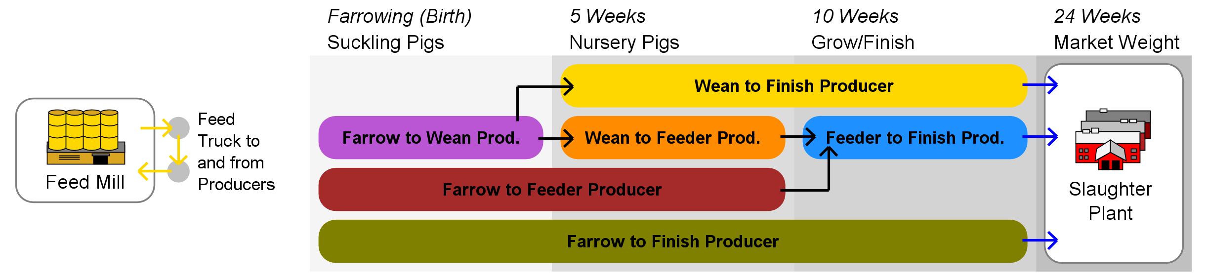
Three types of hog production chain network agents, identified by industry experts as critical players in the transmission of fecal-oral diseases, are represented in the model, these being (a) hog producers, (b) feed mills, and (c) slaughter plants. Producer agents are assigned one of six industry roles based on the classification system used by the USDA and other industry analysts, these being (a) Farrow to Wean, (b) Farrow to Feeder, (c) Farrow to Finish, (d) Wean to Feeder, (e) Wean to Finish, and (f) Feeder to Finish.
The spatial extent of the model is defined by the boundaries of one of three U.S. states: (a) North Carolina, (b) Illinois, or (c) Iowa. These study areas were chosen because each is a major producer of hogs, yet key differences exist regarding the size of their networks and distribution of industry actors, allowing us to incorporate the impact of differences in global network structure into our analysis.
We use the Farm Location and Agricultural Production Simulator (FLAPS) tool—which draws upon USDA Census of Agriculture data along with aerial imaging to impute realistic distributions of livestock farms within a specified U.S. region (Burdett et al. 2015)—to set producer agent locations and key operational parameters including industry roles and capacities. Following FLAPS initialization, each producer generates a list of potential producer trading partners, constrained by maximum distance, size similarity, and maximum number parameters.
Livestock in the model are represented in batches (or metapopulations) of animals of the same age. Producer agents are initialized with one or several pig batches—depending on their capacity—within the correct age range for their industry roles. Farrowing producers periodically generate new piglets, which are subsequently batched as weaner pigs at a rate dependent on their sow inventory, according to industry standards.
Because FLAPS only covers animal production units, feed mill and slaughter plant locations are initialized by distributing them at random positions within each county in proportion to the number of producers in the county, with the overall numbers per state being derived from available datasets in conjunction with expert advisory panels. These non-producer agents are assigned service areas at initialization by having each producer agent connect to the \(n\)th-closest of each type, with \(n\) being drawn from Poisson distributions calibrated in consultation with industry experts. For example, in the case of feed mills, \(\lambda = 1.5\), indicating that a producer is most likely to purchase feed from the first- or second-closest mill, with fewer purchasing from the third-closest, fewer still from the fourth-closest, etc. Alternatively, for slaughter plants, \(\lambda = 2\), indicating that the most likely outcome is for a producer to ship hogs to the second-closest plant. A limitation of RUSH-PNBM is that livestock and feed transfers occur only between model agents; thus, since the model's spatial extent is a single U.S. state, interstate transportation and trade is not represented.
Behavioral heuristics
Agent behavior rules are derived from a review of the primary literature as well as from industry expert advisory panels. A schematic showing the basic interaction flow appears in Figure 1. Livestock are transferred to appropriate agent(s) upon reaching the designated transfer age, and may be split and sent to multiple trading partners. Feed mill agents periodically generate delivery routes that visit a subset of producer agents within their service areas, with the number of deliveries per route being drawn from a Poisson distribution with \(\lambda = 1\).
Epidemiological sub-model
Agents in RUSH-PNBM exist in one of two states: susceptible (S) or infective (I). Infection spread becomes possible whenever a susceptible agent comes into contact with an infective agent. Several modes of inter-agent contact are represented in the model (Figure 1), each corresponding to a potential disease transmission vector within the epidemiological sub-model.
Infected livestock transferred to a susceptible producer automatically infect the recipient. If a susceptible producer transfers livestock to an infective premises, there is a small probability that the infection may be brought back in the form of biological material which has contaminated the transportation equipment. Once a producer agent is infected, it is assumed that its entire premises becomes infected, due to the high reported virulence of PEDv once in a herd (Goede & Morrison 2016). The infection event triggers a mortality calculation that decrements the infected agent’s livestock inventory according to observed mortality rates from PEDv appropriate for the age of each pig batch. Producers remain infective for an average duration of 40 days before transitioning back to susceptible. If a producer ships out its entire livestock inventory, it is assumed that the premises is disinfected prior to receiving a new shipment.
Feed mills may become infected if a delivery truck that has previously been contaminated (by visiting an infective producer) returns to the mill. Mills remain infective for an average of 20 days. While a feed mill is infective, each delivery truck departing the mill may become contaminated. The truck may also become contaminated upon visiting an infective producer part-way through a route. If a contaminated truck visits a susceptible producer, that producer may be infected upon receiving a delivery of contaminated feed.
Slaughter plant receiving areas may become contaminated upon receiving a shipment of infected hogs. The plant’s receiving area will remain infective for an average of five days, during which arriving transportation equipment may become contaminated. Transportation equipment that has been contaminated in this way may then spread the infection upon returning to the originating producer.
To skip the transient period and allow agent interactions to stabilize, the initial infection event, which randomly infects five percent of producer agents, occurs one model year post initialization.
Parameter calibration and validation
Due to the lack of precise animal movement data coupled with the inherent variability of epidemic events within complex networked systems, we are interested less in empirically-validating the model to be used as a forecasting tool, and more in developing sufficient structural- and face-validity to allow for a deeper understanding of the fundamental dynamics of the modeled systems (Klügl 2008). Even given identical starting conditions, deviations in contact patterns over the course of a real-world disease incursion often render precise forecasts unfeasible (Moss 2008). Our aim is rather to uncover and better understand the network features that lead to epidemiological vulnerability in livestock production systems more generally (Epstein 2008).
Calibration procedures that leverage concrete historical data are often regarded as the best way to bring a model in line with empirical evidence. Unfortunately, there is a marked lack of publicly-available data in the agricultural sector beyond aggregated county- or state-level statistics. To the extent that datasets containing explicit locations, operational parameters, livestock and feed movements, and disease histories exist; these data tend to be held by private enterprises, which view them as sensitive internal records. In light of this, following Windrum et al. (2007), we employ several alternative calibration procedures that have been widely-used in previous modeling endeavors in which fine-grained data are scarce.
The spatial locations and basic operational parameters of RUSH-PNBM agents associated with each study area are calibrated using the “indirect” approach, whereby stylized facts about the distribution of agents in the system are gleaned from statistical datasets (Windrum et al. 2007). While the FLAPS tool discussed above (Burdett et al. 2015) serves as our primary means to set agent locations and operational parameters, our team also gained access to internal records from a large family-owned hog production chain system, which are used to codify realistic contact rate and shipment size parameters (see Appendix 1).
Calibration of model elements that define how and when inter-agent contact occurs, as well as epidemiological sub-model parameters, were iteratively honed throughout the model development process following the “companion modeling” approach (Bousquet et al. 1999; Barreteau et al. 2003). During the scoping phase of model development, our research team convened two expert panels that included leading policymakers drawn from industry associations (e.g. the National Pork Board) and the USDA, leading veterinary scientists, Agricultural Extension agents focused on livestock biosecurity from several states, veterinarians working with major livestock production chains, industry communications specialists, and agricultural economists. An additional two panels, involving many of these same experts, were convened during the model’s development. Finally, a fifth expert panel was convened to discuss and interpret the results of the model runs shown here.
In these panel sessions, we used both targeted focus groups as well as quantitative survey questionnaires to elicit and hone parameter values. Through this process, model assumptions, data streams, and behavioral heuristics were shared, critiqued, and refined; and implications of model results were discussed. Detailed notes were taken during these expert panels, which were subsequently coded and analyzed. This information was used to bolster the face-validity of the distribution of epidemic patterns, scales, and durations produced by the model. Using this participatory methodology, the modeled system was brought in line with the collective understandings of stakeholders who are intimately familiar with the operational details of U.S. livestock production chains.
A common perception among our expert panelists concerned the complexity of disease transmission, the variation of disease spread across different states and production chains, and the relatively-meager understanding industry and USDA professionals possesses relative to identifying effective leverage points in production chains that are both most susceptible to disease, and most critical to its spread. Given the complexity of the production chain—with its segmentation of livestock producer roles from farrow to finish—and the importance of feed mills and slaughter plants, industry experts called for the development of an ABM that could capture differences between regions and the configurations of their associated production chain networks.
Sensitivity analysis
We conducted a sensitivity analysis focusing on four key model parameters. While the model includes many parameters (Table 1), these four were chosen because each focuses on a specific aspect of the model’s network and/or epidemiological architecture. Prob. producer to pig truck infection highlights the impact of outgoing disease transmission from a producer agent to either another producer or a slaughter plant. Avg. producer infection length is an infection duration parameter, to which previous SIR-type models have been found to be sensitive. Max producer connection distance evaluates the effect of altering the global network structure from more localized to more spatially-diffused neighborhoods. Finally, Prob. feed truck to feed mill infection aims at elucidating the relative impact of infections stemming from the feed distribution network (versus the livestock transportation network) on system-wide disease resilience.
Each parameter is varied in steps between 50% and 150% of the baseline values given in Table 1, with ten replications per step. Table 2 shows the elasticity of the response variable—average vulnerability—across this range for each study area. Figure 2 visualizes the sensitivity analysis data and provides correlation statistics.
| Change in Avg. Vulnerability | ||||
| Parameter | North Carolina | Iowa | Illinois | All Study Areas |
| Prob. producer to pig truck infection | 49.93 | 109.9 | 491.1 | 94.56 |
| Avg. producer infection length (days) | 2382 | 3164 | 6077 | 3010 |
| Max. producer connection distance (km) | 2.182 | -20.32 | 108.6 | 7.976 |
| Prob. feed truck to feed mill infection | 36.21 | 114.8 | 119.4 | 50.82 |
Results show that the model is moderately-sensitive to changes in Prob. producer to pig truck infection and Prob. feed truck to feed mill infection; with the effect on average vulnerability being positive and significant in all study areas. It would appear that Prob. producer to pig truck infection has a larger impact on the response variable in Illinois, whereas Prob. producer to pig truck infection has the largest impact in North Carolina, reflecting differences in network structure between study areas. Despite state-to-state differences, the fact that increased infectivity in both hog transportation and feed distribution networks both led to similar increases in overall epidemiological vulnerability suggests that our epidemiological spread sub-model is relatively balanced between these two major modes of transmission. This ground-truths our model with respect to real-world findings implicating both contaminated feed and infected hogs/transportation equipment in the spread of PEDv and other diseases (Schulz & Tonsor 2015).
We find that the model is not particularly sensitive to Max producer connection distance. The magnitude and direction of the effect varies between study areas, with only Illinois demonstrating a significant (positive, in this case) relationship to the response variable. While somewhat surprising, this result likely reflects the fact that, despite increasing the Max producer connection distance, the Max. number of potential producer to producer trading partners parameter remained constant (at 15) across all runs. This means that the average (k) of a given producer would only increase with Max producer connection distance in more spatially-diffused networks wherein a sizable proportion of producers did not have 15 potential producer trading partners within the baseline maximum connection distance of 150km. This is more likely to be the case in Illinois, as there are relatively fewer producers within a relatively large area in that state.
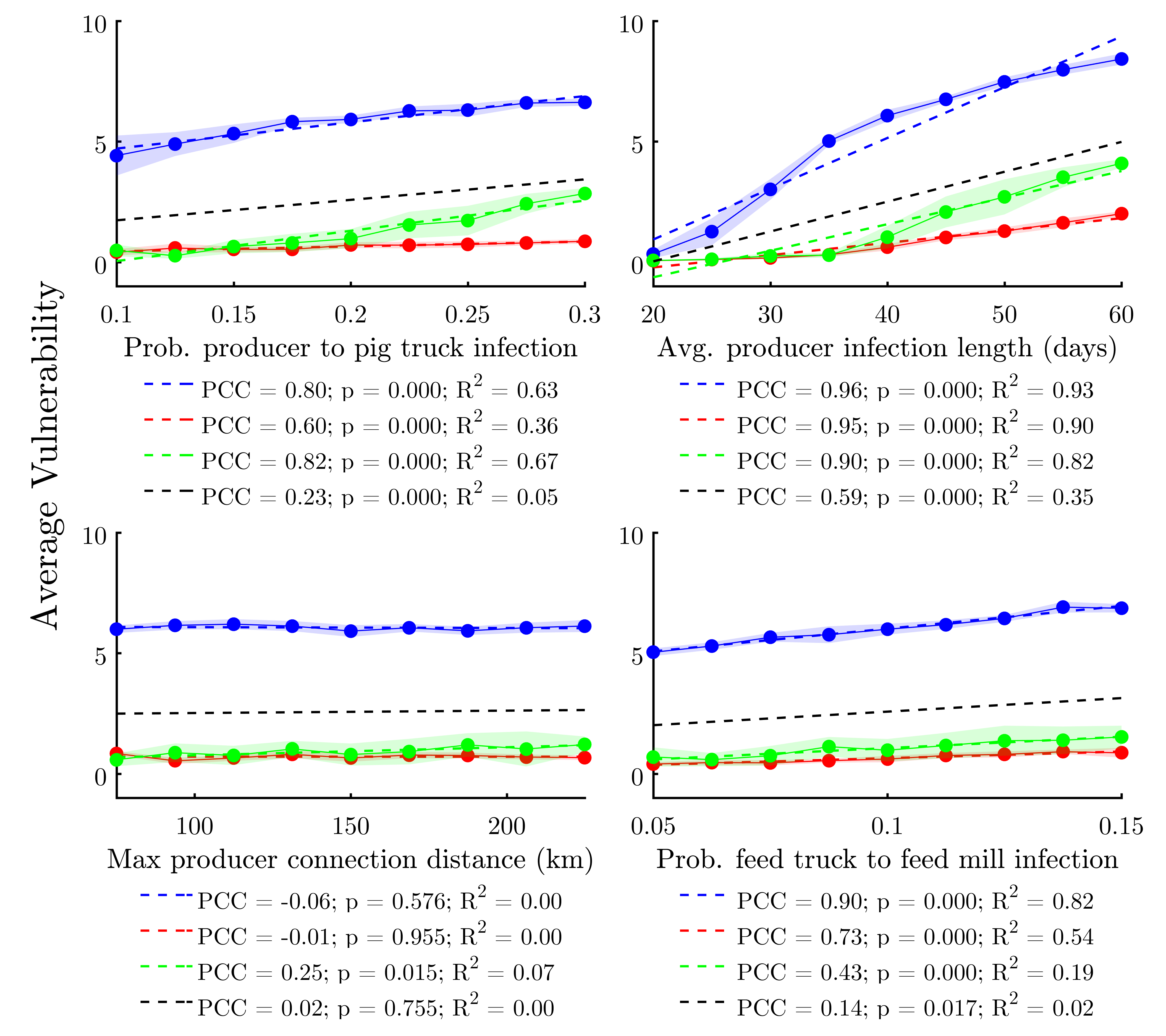
By contrast, increasing Avg. producer infection length causes significant increases in average vulnerability across all study areas. In light of previous SIR/SI model studies, the observation that average infection duration heavily impacts average vulnerability is not a surprise. Further, the shape of the elasticity curves in the top right of Figure 2 suggest that percolation dynamics may exist, with the nonlinearity—or percolation threshold—being lowest for North Carolina and higher for the other two study areas, corroborating findings from Wiltshire (2018).
Experimental Design and Data Processing
The model was executed 50 times for each of the three study areas, maintaining all common parameters constant across repetitions. The total run count of 150 was chosen due to the large number of agents in each study area, along with the relative complexity of the model’s livestock trade and epidemiological spread heuristics, rendering each run—along with its associated data analysis—quite computationally-intensive. The full experimental results encompass 539,300 individual agent-run combinations, with all network metrics and epidemiological statistics calculated for each, yielding a substantially large and rich dataset totaling approximately two million unique datapoints.
The numbers and spatial distributions of each type of agent were hard-coded and maintained across runs within each study area (Table 1). Further, immutable agent properties set at model initialization—including the pool of potential trading partners—were also held across repetitions within each study area. After initialization, all stochastic events in a run utilize a random seed, meaning that—while the underlying network structure associated with each study area production chain remains constant—the transportation of livestock and feed, along with the resultant outbreak progression, is unique from one run to the next.
Throughout each run, a weighted, directed contact network was built up by tracking the number of times each agent contacted another agent—as a result of either delivering or receiving livestock or feed—with the final edge weights being equal to the number of contacts between connected agents. In a similar fashion, an infectivity network was constructed, with edge weights tracking the number of times the infection was passed between agents over the course of a run. An agent’s vulnerability—the dependent variable used in the data analyses below—is defined as a node’s in-degree within the infectivity network.
Networks generated during the experiment, along with key statistics associated with each agent, were output as tabular data at the conclusion of each run. Using the Python NetworkX 2.0 library (Varoquaux et al. 2008), the weighted edgelists describing each network were used to generate weighted, directed network graphs, allowing key global and node-level network metrics previously linked to epidemiological spreading to be evaluated (Ghani & Garnett 2000; Colizza et al. 2007; Webb 2005; Kao et al. 2006; Kiss et al. 2006; Ortiz-Pelaez et al. 2006; Dubé et al. 2009; Bigras-Poulin et al. 2006, 2007; Natale et al. 2009). Where applicable, both weighted and unweighted versions of these metrics were calculated, in order to compare between the two (Rothenberg et al. 1995; Bell et al. 1999). The metrics utilized in this study are listed and briefly described in Table 3. For clarity, we distinguish between the set of node-level metrics pertaining to centrality, versus those capturing other aspects of node positionality. The full sets of global and node metrics used in the analysis were:
| $$global = [\langle k \rangle, \langle k_w \rangle, k^{CV}, k^{CV}_w, \langle C \rangle, \langle C_w \rangle, r, r_w, p^{c_{max}}]$$ | (1) |
| $$node = [k, k_w, k^{in}, k^{in}_w, k^{out}, k^{out}_w, C, C_w, c, C^B, C^B_w, C^{RW}, C^{RW}_w, C^E, C^E_w, C^D]$$ | (2) |
| Description | Ref. | |
| Global Metrics | ||
| UW Average Degree (\(\langle k \rangle\)) | Number of edges divided | (Albert & Barabási 2002) |
| W Average Degree (\(\langle k_w \rangle\)) | Average number of contact events per node per run | (Albert & Barabási 2002) |
| UW Degree CV (\(\langle k^{CV} \rangle\)) | Coefficient of variation for unweighted degree across all nodes | (Newman 2003) |
| W Degree CV (\(\langle k^{CV}_w \rangle\)) | Coefficient of variation for weighted degree across all nodes | (Newman 2003) |
| UW Average Clustering (\(\langle C \rangle\)) | Number of closed triplets divided by total number of triplets | (Luce & Perry 1949) |
| W Average Clustering (\(\langle C_w \rangle\)) | Geometric average of the subgraph edge weights | (Saramäki et al. 2007) |
| UW Assortativity Coefficient (\(\langle r \rangle\)) | Level of similarity between the unweighted degrees of all nodes | (Newman 2003) |
| W Assortativity Coefficient (\(\langle r_w \rangle\)) | Level of similarity between the weighted degrees of all nodes | (Newman 2003) |
| \(k\)-core Fractional Size (\(p^{c_{max}}\)) | Fraction of nodes that are within the main \(k\)-core | (Batagelj & Zaversnik 2003) |
| Node Centrality Metrics | ||
| UW Shortest Path Betweenness (\(C^B\)) | Fraction of shortest-paths passing through a node | (Freeman 1977) |
| W Shortest Path Betweenness (\(C^B_w\)) | Same as above, but incorporating edge weights | (Freeman 1977) |
| UW Random Walk Betweenness (\(C^{RW}\)) | Fraction of random walks passing through a node | (Newman 2005) |
| W Random Walk Betweenness (\(C^{RW}_w\)) | Applies an electric current flow model across all nodes | (Brandes & Fleischer 2005) |
| UW Eigenvector (\(C^E\)) | Nodes connected to other high-\(k\) nodes receive high scores | (Bonacich 1987) |
| & W Eigenvector (\(C^E_w\)) | Same as above, but incorporating edge weights | (Bonacich 1987) |
| Degree (\(C^D\)) | Fraction of nodes to which a node is connected | (Albert & Barabási 2002) |
| Node Positionality Metrics | ||
| UW In-Degree \((k^{in})\) | Number of incoming edges | (Albert & Barabási 2002) |
| W In-Degree \((k_w^{in})\) | Total weight of incoming edges | (Albert & Barabási 2002) |
| UW Out-Degree \((k^{out})\) | Number of outgoing edges | (Albert & Barabási 2002) |
| W Out-Degree \((k_w^{out})\) | Total weight of outgoing edges | (Albert & Barabási 2002) |
| UW Clustering Coefficient \((C)\) | Fraction of possible triangles through a node that exist | (Luce & Perry 1949) |
| W Clustering Coefficient \((C_w)\) | Geometric average of the subgraph edge weights | (Saramäki et al. 2007) |
| Coreness \((c)\) | Largest value \(k\) of a \(k\)-core containing the node | (Batagelj & Zaversnik 2003) |
To generate meta-metrics—that is, formulae composed of multiple individual indicators—we utilized the Eureqa GP package (Schmidt & Lipson 2009). Due to the large size of our dataset, we first sampled the data by randomly selecting 100 agents from each study area to include in the GP training and validation sets. Because of the lower numbers of feed mills and slaughter plants compared to producers, we ensured that all agent types were represented in the data by stipulating that a minimum of five agents of each type from each study area were included, yielding 16,050 total rows. The GP was trained on half of these data (selected randomly) and validated on the remaining half.
The GP algorithm was permitted to use constants, input variables, the four basic arithmetical operators, as well as exponential, logarithmic, and power functions; each of which was assigned a complexity value by which to weigh fitness vs. complexity tradeoffs between potential solutions (Table 4 ).
| Operator | Complexity |
| Constant | 1 |
| Input Variable | 1 |
| Addition | 1 |
| Subtraction | 1 |
| Multiplication | 1 |
| Division | 2 |
| Exponential | 3 |
| Natural Logarithm | 3 |
| Power | 3 |
The objective set for the GP was to maximize the R2 coefficient between the function output and each node’s vulnerability v—at varying levels of complexity—according to the function:
| $$v = f(global, node)$$ | (3) |
The GP was allowed to run until 100% convergence was indicated. The algorithm executed \(1.6 × 10^{10}\) function evaluations over the course of 112,378 generations. 14 total solutions were identified, ranging from \(complexity = 1\) and \(R^2 = 0.04\); to \(complexity = 24\) and \(R^2 = 0.96\).
Results
To analyze our experimental data, we begin by characterizing high-level properties of the production chain networks output by RUSH-PNBM. This allows for a generalized understanding of the similarities and differences between the hog production networks associated with our three study areas, as well as the basic connection patterns and epidemiological vulnerabilities associated with each agent type. Next, we examine the extent to which network metrics can predict individual nodes’ infection vulnerabilities across the three states, examining both network-structural and node positionality factors. Finding that no individual metric adequately correlates with infection risk across study areas, we turn to the GP results to investigate the extent to which formulae composed of multiple metrics—which we call “meta-metrics”—may predict epidemiological vulnerability.
Characterizing study area production networks
Figure 3 shows the degree distributions for each class of agent and study area. Weighted degree (\(k_w\)) represents the number of times an agent contacted another agent (i.e., sending or receiving either livestock or feed) over the course of a run, whereas unweighted degree (\(k\)) describes the number of unique agents with which an agent had contact.
Overall, producers tend to have the lowest \(k_w\) and \(k\), followed in order by feed mills and slaughter plants. Feed mills' degrees are constrained to a smaller range, whereas the distributions for producers and slaughter plants are quite long-tailed. Slaughter plants in Iowa appear to have somewhat higher degrees on average than in the other study areas.
A linear degree distribution in log-log space demonstrates the power law relationship associated with scale-free networks, satisfying \(P[X \geq x] \sim cx^{-\alpha}\) (Barabási & Albert 1999). This appears to be roughly the case for producers, but it is less clear whether the other agent classes exhibit a power law degree distribution.
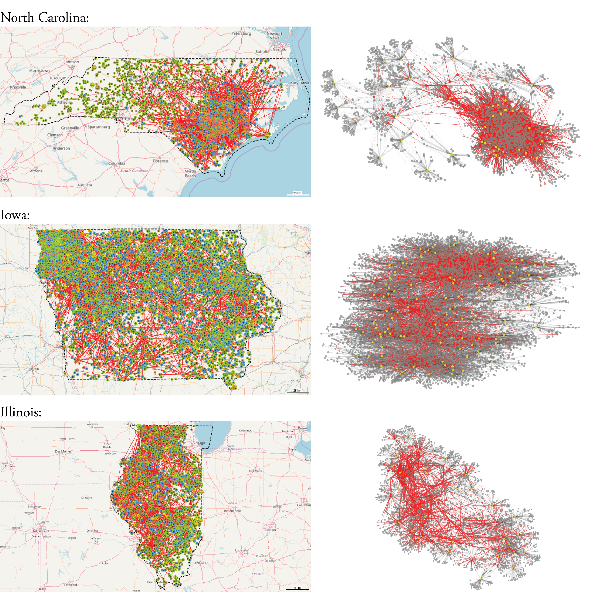
Additionally, we observe that the degree distribution for producers appears to have a different pattern in North Carolina compared with Iowa and Illinois, with North Carolina having more high-\(k\) producers. An examination of Figure 4 suggests that this may be related to the heavily-connected cluster surrounding Duplin County in the southeast of North Carolina.
Table 5 gives epidemiological statistics and key network-structural indicators, averaged by study area. We find notable differences in infection dynamics between study areas, with North Carolina agents having the greatest chance of receiving the infection at least once during a model run, at \(p^{inf} \approx\) 46%, versus 14% for Iowa, and 17% for Illinois. Agents in North Carolina also had the highest average vulnerability (\(\langle v \rangle \approx 6\)), as well as the longest average total infection duration (\(t^{inf} \approx 101\) days).

Examining the averaged network metrics provides some initial insights into these disease resilience discrepancies (Table 1). While the Iowa networks have significantly more nodes, the North Carolina networks are the most densely-connected (higher \(\langle k \rangle\) and \(\langle k_w \rangle\)). Differences are also apparent in the indicators associated with the networks' \(k\)-cores as well as average centrality values. In the sections below, we statistically evaluate the ways in which these patterns in the network data relate to epidemiological vulnerability.
Can network metrics predict infection risk?
Since the probabilities of disease transmission and agents’ behavioral heuristics do not change across runs, the disease risk discrepancies noted above must necessarily result from differences in contact networks. We use a three-pronged approach to analyze the relationships between network structure and epidemic risk factors in the RUSH-PNBM output data. First, we examine the relationships between global metrics that capture overarching features of each study area network, versus the average vulnerability of nodes in these networks, as well as individual agents’ vulnerabilities. Second, we examine the relationships between node-level metrics that capture various aspects of positionality, versus each agent’s vulnerability. Finally, we turn to the GP results to identify meta-metrics that may serve as better indicators of epidemiological risk.
Global network-structural factors
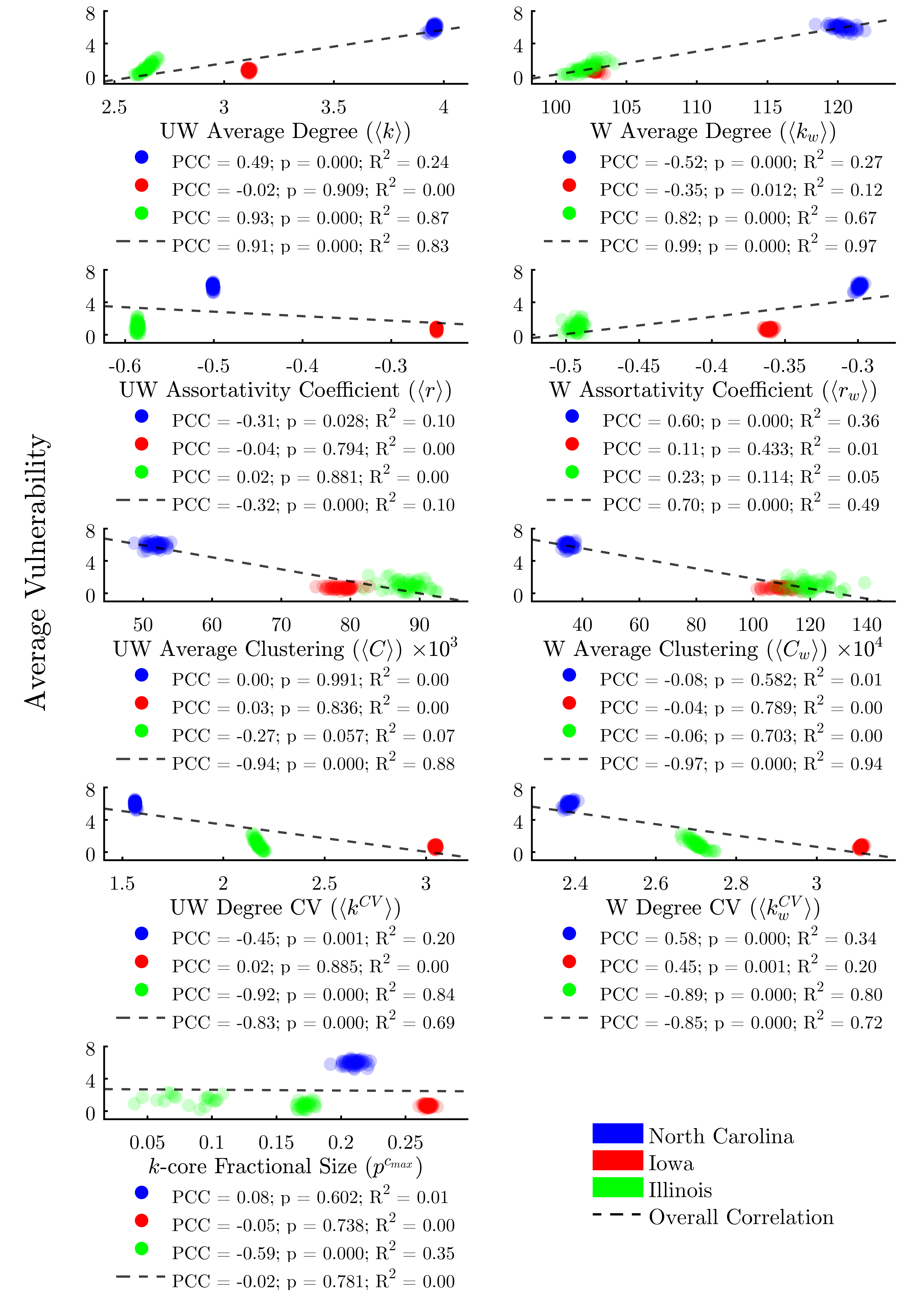
Figure 5 plots the global network metrics described in Table 3 against the average vulnerability of agents in each run. These findings may be analyzed in two ways: first, we can determine whether an overall trend exists across all three study areas; second, we can determine whether a trend exists across the 50 runs associated with each study area. Overall, we find that all global metrics with the exception of (k)-core fractional size do indeed correlate significantly with average vulnerability across all runs.
However, the situation is more complex when examining within-study-area trends. We find that weighted and unweighted average degree, unweighted assortativity, unweighted clustering, weighted and unweighted degree CV, and (k)-core fractional size all exhibit positive correlations in some states and negative in others. Further, the within-state correlations do not achieve significance for several of the metrics. No metric we assessed significantly correlates with average vulnerability both overall as well as within each study area.
While some global network metrics correlate strongly with the average vulnerability of agents in each network, we find that global metrics alone do little to predict the infection risk of individual nodes, owing to the wide range of vulnerabilities between agents. Figure 6 evaluates the same metrics as Figure 5, only this time we plot the individual vulnerability of each agent, rather than per-run averages. Here we find that, in fact, none of the global metrics taken alone is sufficient to explain more than 5% of the variability in the vulnerability of individual agents.
| North Carolina | Iowa | Illinois | |||||||
| Mean | 95% CI | Mean | 95% CI | Mean | 95% CI | ||||
| Epidemiological Statistics | |||||||||
| Vulnerability \((v)\) | 5.949 | 5.833 | 6.064 | 0.6504 | 0.6387 | 0.6620 | 0.9682 | 0.9480 | 0.9883 |
| Infectivity \((i)\) | 5.949 | 5.858 | 6.039 | 0.6504 | 0.6310 | 0.6697 | 0.9682 | 0.9372 | 0.9992 |
| Infection Probability \((p^{inf})\) | 0.4634 | 0.4606 | 0.4663 | 0.1423 | 0.1411 | 0.1435 | 0.1703 | 0.1680 | 0.1725 |
| Spread Probability \((p^{spread})\) | 0.6253 | 0.6225 | 0.6281 | 0.3440 | 0.3424 | 0.3457 | 0.3403 | 0.3374 | 0.3432 |
| Infection Duration \((t^{inf})\) | 101.2 | 100.5 | 101.9 | 14.97 | 14.87 | 15.07 | 19.94 | 19.69 | 20.19 |
| Network Metrics | |||||||||
| Unweighted Degree \((k)\) | 7.910 | 7.838 | 7.982 | 6.226 | 6.161 | 6.292 | 5.298 | 5.228 | 5.367 |
| Weighted Degree \((k_w)\) | 240.6 | 237.3 | 244.0 | 205.4 | 203.2 | 207.6 | 204.3 | 201.0 | 207.6 |
| Unweighted In-Degree \((k^{in})\) | 3.955 | 3.904 | 4.006 | 3.113 | 3.053 | 3.173 | 2.649 | 2.596 | 2.702 |
| Weighted In-Degree \((k_w^{in})\) | 120.3 | 118.8 | 121.8 | 102.7 | 101.4 | 104.0 | 102.1 | 100.9 | 103.4 |
| Unweighted Out-Degree \((k^{out})\) | 3.955 | 3.903 | 4.006 | 3.113 | 3.085 | 3.142 | 2.649 | 2.601 | 2.696 |
| Weighted Out-Degree \((k_w^{out})\) | 120.3 | 117.3 | 123.4 | 102.7 | 100.9 | 104.5 | 102.1 | 98.96 | 105.3 |
| Unweighted Degree CV \((k^{CV})\) | 1.565 | 1.565 | 1.565 | 3.047 | 3.047 | 3.047 | 2.172 | 2.172 | 2.172 |
| Weighted Degree CV \((k^{CV}_w)\) | 2.385 | 2.385 | 2.385 | 3.110 | 3.110 | 3.110 | 2.703 | 2.703 | 2.703 |
| Unweighted Clustering Coefficient \((C)\) | 0.005178 | 0.005049 | 0.005307 | 0.007871 | 0.007723 | 0.008019 | 0.008816 | 0.008554 | 0.009078 |
| Weighted Clustering Coefficient \((C_w)\) | 0.0003497 | 0.0003410 | 0.0003585 | 0.001100 | 0.001078 | 0.001123 | 0.001203 | 0.001165 | 0.001242 |
| Unweighted Assortativity Coefficient \((r)\) | -0.5009 | -0.5009 | -0.5009 | -0.2490 | -0.2490 | -0.2490 | -0.5859 | -0.5859 | -0.5859 |
| Weighted Assortativity Coefficient \((r_w)\) | -0.2989 | -0.2989 | -0.2989 | -0.3610 | -0.3610 | -0.3610 | -0.4931 | -0.4931 | -0.4931 |
| \(k\)-Core Fractional Size \((p^{c_{max}})\) | 0.2101 | 0.2100 | 0.2101 | 0.2673 | 0.2673 | 0.2673 | 0.1380 | 0.1377 | 0.1383 |
| Node Coreness \((c)\) | 4.481 | 4.464 | 4.499 | 3.328 | 3.323 | 3.332 | 2.787 | 2.780 | 2.795 |
| Centrality Indicators | |||||||||
| Unweighted Shortest Path Betweenness \((C^B)\) | 0.001415 | 0.001384 | 0.001447 | 0.0005033 | 0.0004919 | 0.0005147 | 0.001591 | 0.001557 | 0.001625 |
| Weighted Shortest Path Betweenness \((C^B_w)\) | 0.002875 | 0.002805 | 0.002945 | 0.0009989 | 0.0009845 | 0.001013 | 0.003430 | 0.003346 | 0.003513 |
| Unweighted Random Walk Betweenness \((C^{RW})\) | 0.003213 | 0.003161 | 0.003266 | 0.001188 | 0.001172 | 0.001203 | 0.003534 | 0.003476 | 0.003592 |
| Weighted Random Walk Betweenness \((C^{RW}_w)\) | 0.003401 | 0.003341 | 0.003461 | 0.001319 | 0.001300 | 0.001338 | 0.003870 | 0.003800 | 0.003940 |
| Unweighted Eigenvector \((C^E)\) | 0.01379 | 0.01370 | 0.01389 | 0.004814 | 0.004774 | 0.004854 | 0.01565 | 0.01556 | 0.01574 |
| Weighted Eigenvector \((C^E_w)\) | 0.001365 | 0.001244 | 0.001486 | 0.001240 | 0.001197 | 0.001283 | 0.002102 | 0.001971 | 0.002233 |
| Degree \((C^D)\) | 0.003469 | 0.003438 | 0.003501 | 0.0009733 | 0.0009630 | 0.0009836 | 0.002516 | 0.002483 | 0.002549 |
Node positionality factors
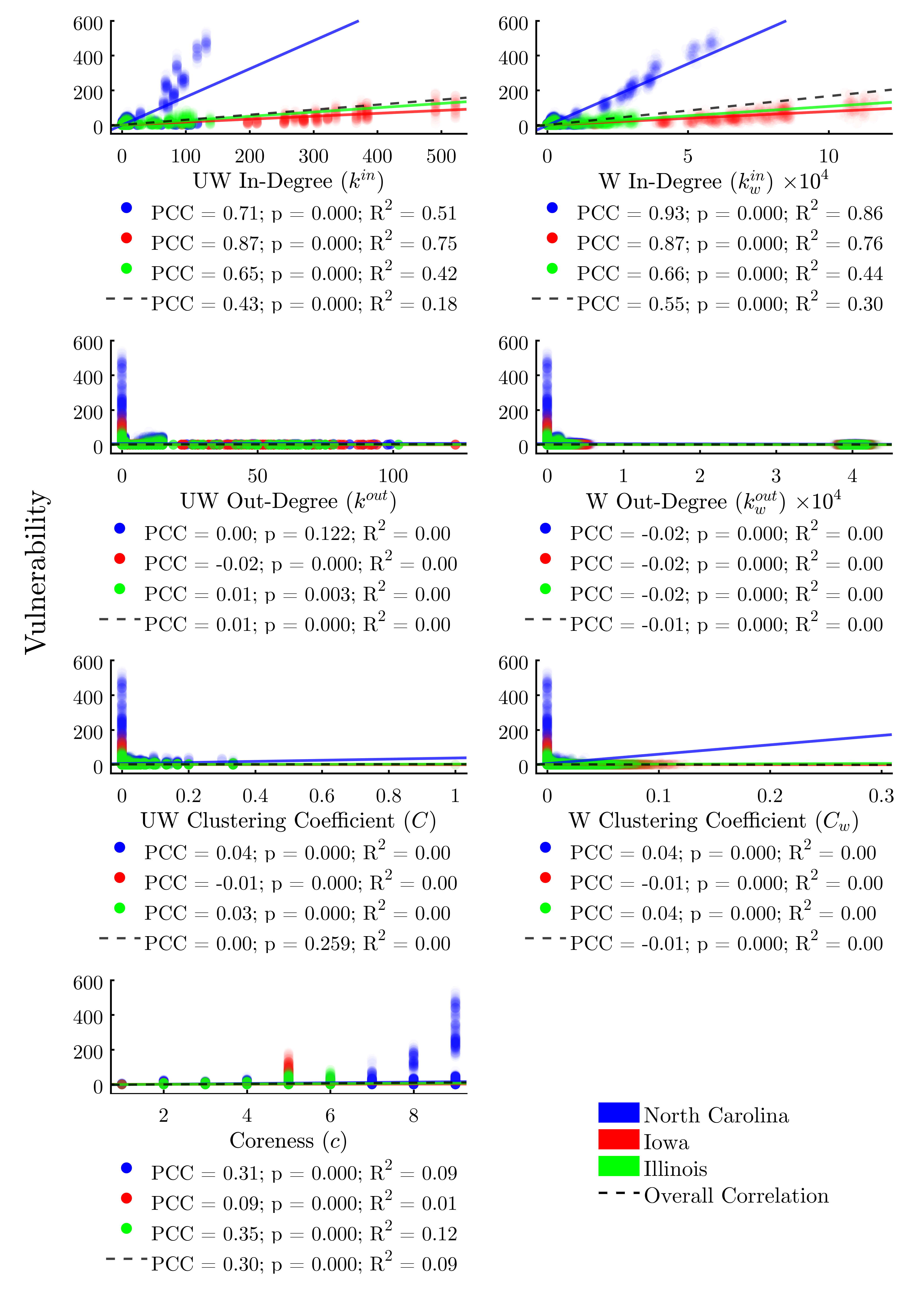
For real-world livestock producers, production system managers, veterinarians, epidemiologists, and policy- makers it would be useful to understand the relationships between the network positionality of a given actor and its risk of infection during an epidemic event. To investigate this, we plot each node-level metric from Table 3 against each agent’s vulnerability. Figure 7 shows the various indicators of node centrality, while Figure 8 shows the remaining node positionality indicators.
We find that all node centrality metrics significantly correlate with infection risk when using the full dataset composed of all three study areas (Figure 7). With the exception of weighted eigenvector, these trends hold within each study area as well. The centrality metric with the most consistent positive correlation to vulnerability across study areas would appear to be degree centrality.
However, linear regressions reveal that, despite achieving significant p-values, no centrality indicator explains more than 22% of the variability in the data across all study areas. Additionally, we find significant variability in the explanatory power of the correlations between study areas. This lends further evidence to the assertion that there is a complex interplay between the structure of a network overall and the efficacy of node-level metrics for determining risk.
Turning to the remaining node positionality indicators (Figure 8), we find—unsurprisingly—that both weighted and unweighted in-degree are relatively-strong predictors of vulnerability, with the weighted metric explaining 30% of the variability in the data. Simply stated, the more times a node is exposed to a potential threat by way of incoming livestock or feed, the more likely it is to be infected. We find that out-degree and clustering coefficient (both weighted and unweighted) do not explain a node’s vulnerability. A node’s coreness is a moderate (R2 = 0.09) predictor of vulnerability across study areas, suggesting that subsets of more highly-interconnected nodes may be largely responsible for sustaining outbreaks.
Using Genetic Programming to develop better vulnerability indicators
Our preliminary findings suggest that, while both global and node-level metrics correlate with epidemiological vulnerability in some contexts, there are likely complexities arising from the interplay between these factors, and no single indicator has a sufficiently high R2 value to be of much use. The development of indicators that consistently identify risk—ideally accounting for both overall network structure and node positionality within a network—would be a boon for epidemiological analysts seeking to target biosecurity interventions in livestock production systems.
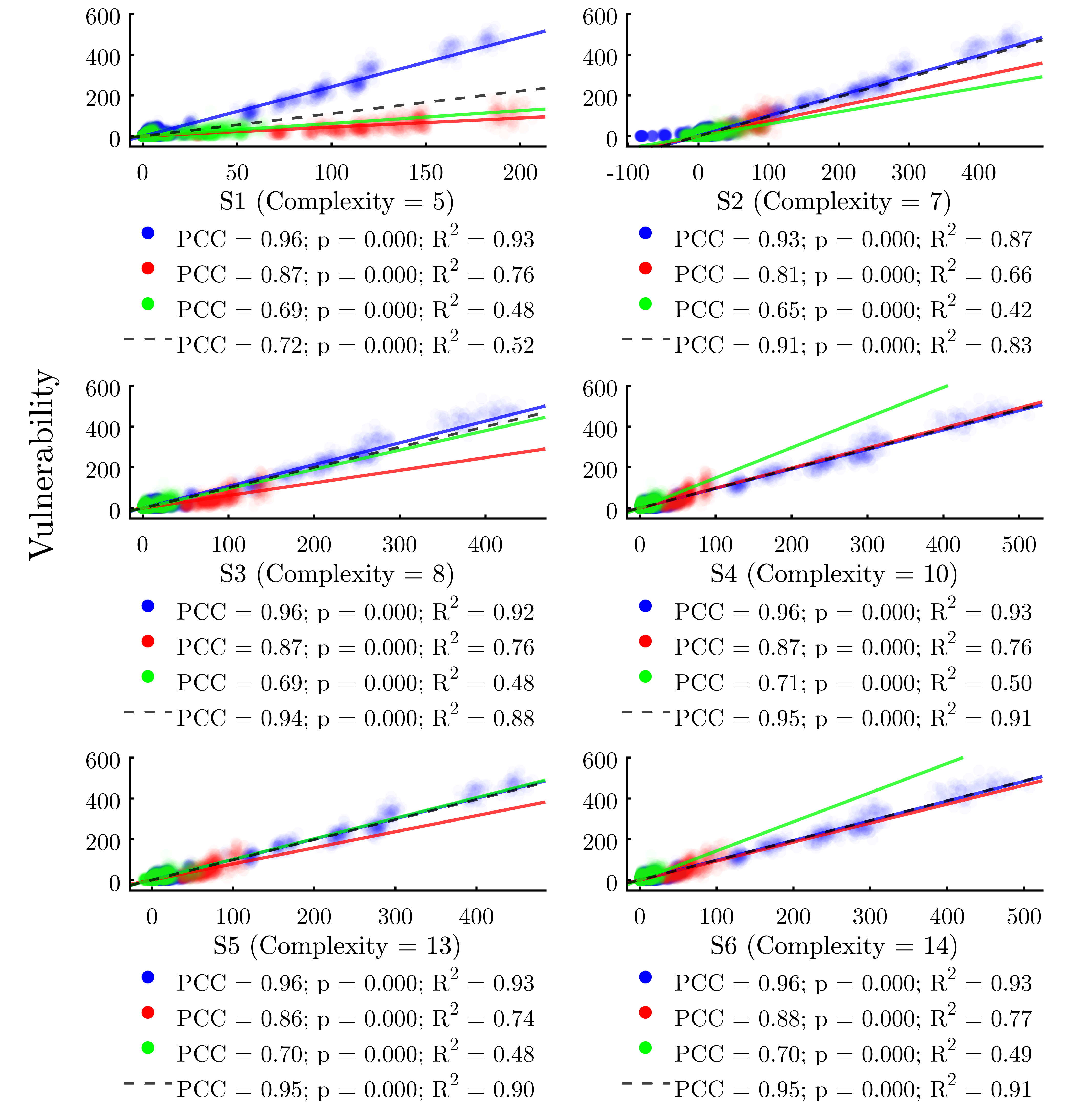
To identify such meta-metrics, we employ a GP algorithm to search the solution space for mathematical combinations of individual indicators along a complexity/fitness Pareto front (Schmidt & Lipson 2009). Of the 14 possible solutions generated by the GP, six were chosen for further analysis (Table 6). This subset of solutions aims to sample a range of complexity/fitness pairings, with solutions situated at “knees” of the Pareto front preferred where possible (Branke et al. 2004). To avoid overfitting the data, solutions beyond a complexity level of 14 are not considered, as there is very little improvement in fitness beyond that point.

Overall, it is notable that the better-performing of the GP solutions incorporate both node-level and global metrics. The most frequently-used node-level metrics are first and foremost weighted in-degree—which is used in all six possible solutions—followed by coreness, unweighted in-degree, unweighted total degree, and weighted eigenvector centrality. The most common (and indeed, only) global metric included in the GP formuae is weighted clustering.

Figure 9 plots the results of the GP solutions against the vulnerability of each node in the same manner as Figures 6, 7, and 8. We find that all of the GP solutions far outperform any individual metric, providing support for the value of the GP-derived meta-metric approach. The best of the GP solutions (S4 and S6) explain 91% of the variability in the response variable, while the best single metric \((k_w^{in})\) explains just 30%.
| Solution | Complexity | R2 | Max. Error | |
| S1 | \(v = 0.0035 \cdot {\color{armygreen}k^{in}_w} \cdot {\color{blue}c}\) | 5 | 0.5496 | 240.8 |
| S2 | \(v = 0.011 \cdot {\color{armygreen}k^{in}_w} \cdot {\color{blue}c} - {\color{armygreen}k^{in}}\) | 7 | 0.9082 | 102.4 |
| S3 | \(v = 2.76 \times 10^{-6} \cdot {\color{armygreen}k^{in}_w} \cdot {\color{blue}c} / {\color{red}\langle C_w \rangle}\) | 8 | 0.9331 | 120.9 |
| S4 | \(v = 3.46 \times 10^{-7} \cdot {\color{armygreen}k^{in}_w} \cdot {\color{blue}c}^2 / {\color{red}\langle C_w \rangle}\) | 10 | 0.9515 | 91.68 |
| S5 | \(v = {\color{armygreen}k^{in}_w} \cdot \left( 0.0010 \cdot {\color{blue}c}^2 - 14.3 \cdot {\color{red}\langle C_w \rangle} \right)\) | 13 | 0.9531 | 83.64 |
| S6 | \(v = {\color{armygreen}k^{in}} \cdot {\color{blue}C^{E}_w} + 3.42 \times 10^{-7} \cdot {\color{armygreen}k^{in}_w} \cdot {\color{blue}c}^2 / {\color{red}\langle C_w \rangle} \) | 14 | 0.9562 | 75.79 |
Discussion and Conclusions
In this study, we apply agent-based computer modeling, network analytics, and evolutionary computation to explore the impact of key network metrics on the epidemiological vulnerability of livestock production chain actors. We analyze the extent to which indicators describing the structure of a complex contact network can be combined with those pertaining to a node’s positionality within that network to arrive at better risk indicators. To this end, we demonstrate the feasibility of using a GP algorithm to formulate such meta-metrics and, at least in this context, we find that the GP solutions outperform any single indicator of epidemiological vulnerability. Below, we discuss how the meta-metric method could be used by real-world practitioners, address methodological issues surrounding data availability and context specificity, and propose future research goals.
Previous research in this area has largely explored bivariate correlations between of a suite of metrics and epidemiological outcomes—at either the network or individual level—in both simulated and real-world networked systems (Rothenberg et al. 1995; Bell et al. 1999; De et al. 2004; Christley et al. 2005; Salathé & Jones 2010; Kitsak et al. 2010). Multivariate statistical techniques have also been used to evaluate the relative effect of multiple node-level metrics on individual vulnerability (Ghani & Garnett 2000). The GP methodology we have employed expands on this work, searching the solution space to identify mathematical relationships encompassing multiple metrics to predict a node’s vulnerability across three networks with differing sizes, densities, and internal structures.
The ability of our GP approach to identify meta-metrics that capture complexities arising from the interactions between global and node-level network features suggests that this methodology may have widespread applicability. The particular networks evaluated in this experiment were state-level livestock production systems generated by a computer model, but we believe the procedures used to analyze the network data and identify meta-metrics could be applied to study phenomena on a wide range of graphs, both empirically- and computationally-derived. While we have applied the meta-metric approach to study epidemiological dynamics, meta-metrics could equally be formulated to predict other important graph properties, such as the probability that a node will add or prune edges over time, the frequency with which a node will enter some state, or virtually any other outcome variable of interest.
Global vs. node metrics as indicators of vulnerability
We find that the global metrics, while serving as reasonably-accurate predictors of average vulnerability within each study area, do little to predict the risk of an individual agent within each run, as a result of the high variability in vulnerability across agents of different classes, and with different network positionality characteristics (Figure 6).
Several of the node-level metrics, such as degree centrality and weighted in-degree, perform reasonably well as predictors of an agent’s vulnerability (R2 = 0.22 and 0.30 respectively). However, many of the node metrics demonstrate differential correlation coefficients across each study area, indicating that risk cannot be accurately predicted by node-level indicators alone (Figures 7 and 8).
Evaluating GP-derived meta-metrics
Turning to the GP solutions, we find that the best-performing meta-metrics (S3–S6) incorporate both global and node-level indicators. Further, among the node metrics, we note that some of the calculations—for example weighted in-degree—require only local information from each node for calculation (indicated in green in Table 6). However, other node metrics—for example coreness—require that a full graph of the network is first codified (indicated in blue in Table 6). Notably, all six of the GP solutions we analyzed do require at least one instance of a node metric that falls into this latter category (primarily coreness in this case), emphasizing the interplay between global network structures and node positionality in the prediction of infection risk.
Weighing the six meta-metric solutions against one another, S4 and S6 are the best performing of the set, each achieving a high overall R2 value of 0.91 on the full dataset. Table 6 reveals that S6, while more complex, cuts the maximum error from 91.68 for S4 to 75.79 for S6, suggesting that the additional complexity pays off in terms of predictive accuracy in this context. Overall, we conclude that the GP approach to determining effective predictors of epidemiological risk by combining indicators of network structure with node positionality represents an effective and under-explored mechanism to evaluate the infection vulnerability of individual nodes within networks.
Application to real-world decision-making
Aside from demonstrating the applicability of our methodology, this work is also intended to inform practitioners in their efforts to strategically-allocate resources which improve epidemiological resilience in existing livestock production systems. While we do not wish to imply that the results presented here can reliably predict the course of any real-world disease incursion, our findings suggest several novel ways for livestock epidemiologists to approach risk analysis.
Perhaps the most important takeaway from our study is that risk is a function of both network structure and individual decision-making. Biosecurity measures—such as shower-in-shower-out facilities, lines of separation, or all-in-all-out protocols—have proven effective in limiting the scope of livestock disease outbreaks. While a producer’s primary motivation to adopt such measures is rooted in individual risk reduction, from a systems perspective, our research suggests that biosecurity protocols would be vastly more effective if implemented at especially-vulnerable network loci. The methods presented in this study allow for the identification of nodes in a system most likely to play a role in disease spread, which can then inform targeted biosecurity interventions to reduce systemic risk.
The lack of available fine-grained U.S. animal movement data currently represents a major hurdle for network analysts and modelers interested in livestock disease risk mitigation. Animal traceback protocols, which track the movement of livestock between premises over their full lifespans, remain controversial in the U.S., likely due to attitudes around privacy. While consumer protection (recalls, etc.) is the most-cited reason for the implementation of traceback protocols, in light of our findings, an additional consideration is that traceback data could be used to codify accurate network representations of livestock supply chains, as has been done in other countries (Caporale et al. 2001; Natale et al. 2009).
Given sufficient input data, RUSH-PNBM could be parameterized to guide on-the-ground policy and managerial decisions. By encoding the interaction patterns and animal movements between actors in real-world production systems into network graphs, and then incorporating data tracking the spread of a historical outbreak through the system, it becomes possible to apply the methods we have presented to actual disease incursion threat scenarios.
Model use cases could focus on different scales. For example, national agencies such as the USDA could use RUSH-PNBM to target nationwide interventions—such as the placement of truck-wash sites—or to propose health and safety regulations focused on potential “hubs” like slaughter plants and feed mills. Alternatively, owners and managers of private livestock production chain systems could employ specifically-parameterized versions of the model to assess disease risks within their own systems. This would facilitate both insights into the individual network loci at which biosecurity protocols could do the most good, as well as analyses of how reorganization of network structures could improve system-wide disease resilience.
Expert panelist feedback
The variation of individual node vulnerabilities found in our results did not surprise our panelists: the relation- ship between an individual node’s vulnerability and its position and/or function in the network matters. The potential of our model to identify those nodes with the highest disease risk casts light on an important informational need raised in our panel sessions. Coupled with finer-grained and more-detailed data (such as the widespread use of animal traceback protocols), panelists agreed that RUSH-PNBM—together with the meta-metric methodology—could represent a valuable tool which may be leveraged to identify where best to target biosecurity measures.
Interestingly, many of the expert panelists were less interested in some of the broader structural implications that may be drawn from this study. For example, despite its demonstrated biosecurity implications, minimizing the bridging links within livestock production networks by reducing producer over-specialization was not universally deemed desirable. However, more recent engagement between our research team and owners of mid-sized, leading-edge production chain systems has revealed an openness to rethinking the role of network connectivity structures upon biosecurity within the context of their own operational networks.
Limitations of our approach
Macro-scale socio-economic and political factors can directly and indirectly influence the economic incentives, disease patterns, and network-structural parameters embedded in RUSH-PNBM. While this study demonstrates the limited generalizability of our model across three states in the U.S., application of the model to other socio- economic and political contexts (e.g. the EU) will require careful re-calibration and validation of model parameters, including securing relevant datasets and convening additional expert panels. Extensibility of RUSH-PNBM to generate medium- to long-term (i.e. 30- to 50-year) scenarios would also require refinement of simulation processes and parameters to account for projected changes in economic and political conditions within which the simulated networks operate.
As noted above, practical implementation of this new meta-metric approach (i.e. to guide policymaking) will require better contextualization of the network structures and underlying theoretical assumptions governing network dynamics. Due to complex government-industry relationships and competition within the livestock production industry, empirical data concerning underlying network structures, animal movements, epidemic spread data, and other important factors are not typically easily available. Fortunately, ABMs—acting as virtual laboratories (Macal & North 2010)—enable testing of alternate assumptions about network structures and their underlying dynamics. As described above, widespread adoption of animal traceback protocols would go a long way toward solving the data availability issue.
Directions for future research
Previous studies investigating the impact of network positionality on epidemiological risk differentiate between vulnerability—which we have used as our dependent variable—and infectivity, i.e. the frequency with which an actor spreads the disease to others (Rothenberg et al. 1995; Ghani & Garnett 2000). Understanding both factors is important to guide the implementation of interventions which curb disease spread, as some protocols are designed to prevent incoming disease threats, whereas others are aimed at limiting outgoing infection spread. An area for future research is to develop GP-derived meta-metrics that correlate with a node’s infectivity rather than its vulnerability. For example, it would be interesting to determine whether the finding of Ghani & Garnett (2000)—that infectivity is more contingent on global network structures—is corroborated. This would offer a more complete picture of the overall risk environment.
In addition, future versions of the RUSH-PNBM model itself will be increasingly honed. For example, our team will conduct survey research to evaluate the economic and human dimensions underlying choices to adopt methods and technologies aimed at bolstering producer-level biosecurity. Another future research goal is to use experimental gaming data to determine the circumstances under which individuals choose to adopt biosecurity protocols in risky and/or uncertain decision environments (Merrill et al. 2019). We can then program the agents in RUSH-PNBM to adapt their behavior under parallel conditions in the model. Coupling such insights with network-based risk analyses—especially those calibrated around real-world production chain systems—will allow for a deeper understanding of the human-behavioral solutions that may promote the adoption of risk-mitigating protocols, as well as helping to focus biosecurity protocol adoption upon the nodes at which it will have the greatest effect on system-wide disease resilience.
Acknowledgements
This material is based upon work that is supported by the National Institute of Food and Agriculture, U.S. Department of Agriculture, under award number 2015-69004-23273. Any opinions, findings, conclusions, or recommendations expressed in this publication are those of the author(s) and do not necessarily reflect the view of the U.S. Department of Agriculture. The funders had no role in study design, data collection and analysis, decision to publish, or preparation of the manuscript.References
ALBERT, R. & Barabási, A.-L. (2002). Statistical mechanics of complex networks. Reviews of Modern Physics, 74(1), 47. [doi:10.1103/RevModPhys.74.47]
ALDERTON, S., Macleod, E. T., Anderson, N. E., Schaten, K., Kuleszo, J., Simuunza, M., Welburn, S. C. & Atkinson, P. M. (2016). A multi-host agent-based model for a zoonotic, vector-borne disease: A case study on trypanosomiasis in eastern province, Zambia. PLoS Neglected Tropical Diseases, 10(12), e0005252.
AN, L. (2012). Modeling human decisions in coupled human and natural systems: Review of agent-based models. Ecological Modelling, 229, 25–36. [doi:10.1016/j.ecolmodel.2011.07.010]
ANDERSON, R. M. & May, R. M. (1979). Population biology of infectious diseases: Part I. Nature, 280(5721), 361.
ARRUDA, A. G., Friendship, R., Carpenter, J., Greer, A. & Poljak, Z. (2016). Evaluation of control strategies for porcine reproductive and respiratory syndrome (PRRS) in swine breeding herds using a discrete event agent- based model. PLoS ONE, 11(11), e0166596. [doi:10.1371/journal.pone.0166596]
AUCHINCLOSS, A. H. & Diez Roux, A. V. (2008). A new tool for epidemiology: The usefulness of dynamic-agent models in understanding place effects on health. American Journal of Epidemiology, 168(1), 1–8.
BAGNI, R., Berchi, R. & Cariello, P. (2002). A comparison of simulation models applied to epidemics. Journal of Artificial Societies and Social Simulation, 5(3), 5: https://www.jasss.org/5/3/5.html.
BARABÁSI, A.-L. & Albert, R. (1999). Emergence of scaling in random networks. Science, 286(5439), 509–512.
BARRETEAU, O., Antona, M., D’Aquino, P., Aubert, S., Boissau, S., Bousquet, F., Daré, W., Etienne, M., Le Page, C., Mathevet, R. et al. (2003). Our companion modelling approach. Journal of Artificial Societies and Social Simulation, 6(2), 1: https://www.jasss.org/6/2/1.html.
BARRETT, C. L., Bisset, K. R., Eubank, S. G., Feng, X. & Marathe, M. V. (2008). Episimdemics: An efficient algorithm for simulating the spread of infectious disease over large realistic social networks. In High Performance Computing, Networking, Storage and Analysis, (pp. 1–12). IEEE Austin, TX.
BATAGELJ, V. & Zaversnik, M. (2003). An o (m) algorithm for cores decomposition of networks. arXiv preprint cs/0310049.
BELKHIRIA, J., Alkhamis, M. A. & Martínez-López, B. (2016). Application of species distribution modeling for avian influenza surveillance in the United States considering the north America migratory flyways. Nature Scientific Reports, 6, 33161.
BELL, D. C., Atkinson, J. S. & Carlson, J. W. (1999). Centrality measures for disease transmission networks. Social Networks, 21(1), 1–21. [doi:10.1016/S0378-8733(98)00010-0]
BIGRAS-POULIN, M., Barfod, K., Mortensen, S. & Greiner, M. (2007). Relationship of trade patterns of the Danish swine industry animal movements network to potential disease spread. Preventive Veterinary Medicine, 80(2-3), 143-165.
BIGRAS-POULIN, M., Thompson, R., Chriél, M., Mortensen, S. & Greiner, M. (2006). Network analysis of Danish cattle industry trade patterns as an evaluation of risk potential for disease spread. Preventive Veterinary Medicine, 76(1), 11–39. [doi:10.1016/j.prevetmed.2006.04.004]
BONACICH, P. (1987). Power and centrality: A family of measures. American Journal of Sociology, 92(5), 1170–1182.
BOUSQUET, F., Barreteau, O., Le Page, C., Mullon, C. & Weber, J. (1999). An environmental modelling approach: The use of multi-agent simulations. Advances in Environmental and Ecological Modelling, 113, 122.
BRADHURST, R., Roche, S. E., East, I., Kwan, P. & Garner, M. (2016). Improving the computational efficiency of an agent-based spatiotemporal model of livestock disease spread and control. Environmental Modelling & Software, 77, 1–12.
BRANDES, U., & Fleischer, D. (2005, February). ‘Centrality measures based on current flow.’ In V. Diekert and B. Durand (Eds.), Annual symposium on theoretical aspects of computer science. Berlin/Heidelberg: Springer, pp. 533-544. [doi:10.1007/978-3-540-31856-9_44]
BRANKE, J., Deb, K., Dierolf, H. & Osswald, M. (2004). ‘Finding knees in multi-objective optimization.’ In in X. Yao et al. (Eds.), International conference on parallel problem solving from nature. Berlin/Heidelberg: Springer, pp. 722–731.
BURDETT, C. L., Kraus, B. R., Garza, S. J., Miller, R. S., & Bjork, K. E. (2015). Simulating the distribution of individual livestock farms and their populations in the United States: An example using domestic swine (Sus scrofa domesticus) farms. PLoS ONE, 10(11), e0140338. [doi:10.1371/journal.pone.0140338]
CAPORALE, V., Giovannini, A., Di Francesco, C., & Calistri, P. (2001). Importance of the traceability of animals and animal products in epidemiology. Revue Scientifique et Technique-Office International des Epizooties, 20(2), 372-378.
CHRISTLEY, R. M., Pinchbeck, G., Bowers, R., Clancy, D., French, N., Bennett, R. & Turner, J. (2005). Infection in social networks: Using network analysis to identify high-risk individuals. American Journal of Epidemiology, 162(10), 1024–1031 [doi:10.1093/aje/kwi308]
COLIZZA, V., Barrat, A., Barthélemy, M. & Vespignani, A. (2007). Predictability and epidemic pathways in global outbreaks of infectious diseases: the SARS case study. BMC Medicine, 5(1), 34.
DE, P., Singh, A. E., Wong, T., Yacoub, W. & Jolly, A. (2004). Sexual network analysis of a gonorrhoea outbreak. Sexually Transmitted Infections, 80(4), 280–285. [doi:10.1136/sti.2003.007187]
DUBÉ, C., Ribble, C., Kelton, D. & McNab, B. (2009). A review of network analysis terminology and its application to foot-and-mouth disease modelling and policy development. Transboundary and Emerging Diseases, 56(3), 73–85.
EL-SAYED, A. M., Scarborough, P., Seemann, L. & Galea, S. (2012). Social network analysis and agent-based modeling in social epidemiology. Epidemiologic Perspectives & Innovations, 9(1), 1. [doi:10.1186/1742-5573-9-1]
EPSTEIN, J. M. (2008). Why model? Journal of Artificial Societies and Social Simulation, 11(4), 12: https://www.jasss.org/11/4/12.html.
FÈVRE, E. M., Bronsvoort, B. M. d. C., Hamilton, K. A. & Cleaveland, S. (2006). Animal movements and the spread of infectious diseases. Trends in Microbiology, 14(3), 125–131. [doi:10.1016/j.tim.2006.01.004]
FREEMAN, L. C. (1977). A set of measures of centrality based on betweenness. Sociometry, 35-41.
GARNER, M. & Hamilton, S. (2011). Principles of epidemiological modelling. Revue scientifique et technique–OIE, 30(2), 407. [doi:10.20506/rst.30.2.2045]
GARNER, M. G., Dubé, C., Stevenson, M. A., Sanson, R. L., Estrada, C. & Griuin, J. (2007). Evaluating alternative approaches to managing animal disease outbreaks–the role of modelling in policy formulation. Veterinaria Italiana, 43(2), 285–298.
GHANI, A. C. & Garnett, G. P. (2000). Risks of acquiring and transmitting sexually transmitted diseases in sexual partner networks. Sexually Transmitted Diseases, 27(10), 579–587. [doi:10.1097/00007435-200011000-00006]
GOEDE, D., & Morrison, R. B. (2016). Production impact & time to stability in sow herds infected with porcine epidemic diarrhea virus (PEDV). Preventive veterinary medicine, 123, 202-207.
HARVEY, N., Reeves, A., Schoenbaum, M. A., Zagmutt-Vergara, F. J., Dubé, C., Hill, A. E., Corso, B. A., McNab, W. B., Cartwright, C. I. & Salman, M. D. (2007). The North American animal disease spread model: A simulation model to assist decision making in evaluating animal disease incursions. Preventive Veterinary Medicine, 82(3-4), 176–197. [doi:10.1016/j.prevetmed.2007.05.019]
HUNTER, E., Mac Namee, B. & Kelleher, J. D. (2017). A taxonomy for agent-based models in human infectious disease epidemiology. Journal of Artificial Societies and Social Simulation, 20(3), 2: https://www.jasss.org/20/3/2.html. [doi:10.18564/jasss.3414]
KAO, R., Danon, L., Green, D. & Kiss, I. (2006). Demographic structure and pathogen dynamics on the network of livestock movements in Great Britain. Proceedings of the Royal Society of London B: Biological sciences, 273(1597), 1999–2007. [doi:10.1098/rspb.2006.3505]
KAUL, H. & Ventikos, Y. (2013). Investigating biocomplexity through the agent-based paradigm. Briefings in Bioinformatics, 16(1), 137–152.
KILLWORTH, P. D., McCarty, C., Bernard, H. R., Shelley, G. A. & Johnsen, E. C. (1998). Estimation of seroprevalence, rape, and homelessness in the United States using a social network approach. Evaluation Review, 22(2), 289– 308. [doi:10.1177/0193841X9802200205]
KISS, I. Z., Green, D. M. & Kao, R. R. (2006). The network of sheep movements within Great Britain: Network properties and their implications for infectious disease spread. Journal of the Royal Society Interface, 3(10), 669–677.
KITCHING, R. P., Thrusfield, M. V., & Taylor, N. M. (2006). Use and abuse of mathematical models: an illustration from the 2001 foot and mouth disease epidemic in the United Kingdom. Revue Scientifique et Technique-Office International des Epizooties, 25(1), 293. [doi:10.20506/rst.25.1.1665]
KITSAK, M., Gallos, L. K., Havlin, S., Liljeros, F., Muchnik, L., Stanley, H. E. & Makse, H. A. (2010). Identification of influential spreaders in complex networks. Nature Physics, 6(11), 888–893.
KLÜGL, F. (2008). A validation methodology for agent-based simulations. In Proceedings of the 2008 ACM Symposium on Applied Computing, (pp. 39–43). ACM. [doi:10.1145/1363686.1363696]
LUCE, R. D. & Perry, A. D. (1949). A method of matrix analysis of group structure. Psychometrika, 14(2), 95–116
MACAL, C. & North, M. (2010). Tutorial on agent-based modelling and simulation. Journal of Simulation, 4(3), 151–162. [doi:10.1057/jos.2010.3]
MANSLEY, L., Dunlop, P., Whiteside, S. & Smith, R. (2003). Early dissemination of foot-and-mouth. The Veterinary Record, 153, 43–50.
MERRILL, S. C., Koliba, C. J., Zia, A., Parker, J., Moegenburg, S., Sellnow, T., Wiltshire, S. W., Bucini, G., Danehy, C. & Smith, J. M. (2019). Adoption of livestock biosecurity practices amidst environmental and social uncertainty: Evidence from a randomized experimental game. PLoS ONE, 14(4): e0214500.. Under Review. [doi:10.1371/journal.pone.0214500]
MOSS, S. (2008). Alternative approaches to the empirical validation of agent-based models. Journal of Artificial Societies and Social Simulation, 11(1), 5: https://www.jasss.org/11/1/5.html.
NATALE, F., Giovannini, A., Savini, L., Palma, D., Possenti, L., Fiore, G. & Calistri, P. (2009). Network analysis of Italian cattle trade patterns and evaluation of risks for potential disease spread. Preventive Veterinary Medicine, 92(4), 341–350. [doi:10.1016/j.prevetmed.2009.08.026]
NEWMAN, M. E. (2003). Mixing patterns in networks. Physical Review E, 67(2), 026126.
NEWMAN, M. E. (2005). A measure of betweenness centrality based on random walks. Social Networks, 27(1), 39–54. [doi:10.1016/j.socnet.2004.11.009]
ORTIZ-PELAEZ, A., Pfeiuer, D., Soares-Magalhaes, R. & Guitian, F. (2006). Use of social network analysis to characterize the pattern of animal movements in the initial phases of the 2001 foot and mouth disease (FMD) epidemic in the UK. Preventive Veterinary Medicine, 76(1-2), 40–55.
PARKER, J. & Epstein, J. M. (2011). A distributed platform for global-scale agent-based models of disease transmission. ACM Transactions on Modeling and Computer Simulation (TOMACS), 22(1), 2. [doi:10.1145/2043635.2043637]
PEREZ, A. M., Ward, M. P., Charmandarián, A. & Ritacco, V. (2002). Simulation model of within-herd transmission of bovine tuberculosis in argentine dairy herds. Preventive Veterinary Medicine, 54(4), 361–372.
PEREZ, L. & Dragicevic, S. (2009). An agent-based approach for modeling dynamics of contagious disease spread. International Journal of Health Geographics, 8(1), 50. [doi:10.1186/1476-072X-8-50]
ROBINS, J., Bogen, S., Francis, A., Westhoek, A., Kanarek, A., Lenhart, S. & Eda, S. (2015). Agent-based model for Johne’s disease dynamics in a dairy herd. Veterinary Research, 46(1), 68.
ROTHENBERG, R. B., Potterat, J. J., Woodhouse, D. E., Darrow, W. W., Muth, S. Q. & Klovdahl, A. S. (1995). Choosing a centrality measure: Epidemiologic correlates in the Colorado Springs study of social networks. Social Networks, 17(3-4), 273–297. [doi:10.1016/0378-8733(95)00267-R]
SALATHÉ, M. & Jones, J. H. (2010). Dynamics and control of diseases in networks with community structure. PLoS Computational Biology, 6(4), e1000736.
SARAMÄKI, J., Kivelä, M., Onnela, J.-P., Kaski, K. & Kertesz, J. (2007). Generalizations of the clustering coefficient to weighted complex networks. Physical Review E, 75(2), 027105. [doi:10.1103/PhysRevE.75.027105]
SCHMIDT, M. & Lipson, H. (2009). Distilling free-form natural laws from experimental data. Science, 324(5923), 81–85.
SCHOENBAUM, M. A. & Disney, W. T. (2003). Modeling alternative mitigation strategies for a hypothetical outbreak of foot-and-mouth disease in the United States. Preventive Veterinary Medicine, 58(1-2), 25–52. [doi:10.1016/S0167-5877(03)00004-7]
SCHULZ, L. L. & Tonsor, G. T. (2015). Assessment of the economic impacts of porcine epidemic diarrhea virus in the United States. Journal of Animal Science, 93(11), 5111–5118.
SHI, Z. Z., Wu, C.-H. & Ben-Arieh, D. (2014). Agent-based model: A surging tool to simulate infectious diseases in the immune system. Open Journal of Modelling and Simulation, 2(01), 12. [doi:10.4236/ojmsi.2014.21004]
STEVENSON, M., Sanson, R., Stern, M., O’Leary, B., Sujau, M., Moles-Benfell, N. & Morris, R. (2013). Interspread plus: A spatial and stochastic simulation model of disease in animal populations. Preventive Veterinary Medicine, 109(1-2), 10–24
THE Pig Site (2014). Pig farm targets: Stockmanship standards. Archived by WebCite at http://www.webcitation.org/6ypMDxs0e.
TRACEY, J. A., Bevins, S. N., VandeWoude, S. & Crooks, K. R. (2014). An agent-based movement model to assess the impact of landscape fragmentation on disease transmission. Ecosphere, 5(9), 1–24.
USDA NASS (2014). Livestock slaughter, 2013 summary: Federally inspected plants and head slaughtered by species, states and United States, 2013. Archived by WebCite at http://www.webcitation.org/6ypM8s3hf URL http://usda.mannlib.cornell.edu/usda/nass/LiveSlauSu/2010s/2014/LiveSlauSu-04-21-2014.pdf.
VAROQUAUX, G., Vaught, T. & Millman, J. (Eds.) (2008). Exploring network structure, dynamics, and function using NetworkX. Pasadena, CA USA: Proceedings of the 7th Python in Science Conference (SciPy2008).
WASSERMAN, S.& Faust, K. (1994). Social Network Analysis: Methods and Applications (Vol. 8) Cambridge, MA: Cambridge University Press. [doi:10.1017/CBO9780511815478]
WEBB, C. R. (2005). Farm animal networks: Unraveling the contact structure of the British sheep population. Preventive Veterinary Medicine, 68(1), 3–17.
WILTSHIRE, S. W. (2018). Using an agent-based model to evaluate the effect of producer specialization on the epidemiological resilience of livestock production networks. PloS ONE, 13(3), e0194013. [doi:10.1371/journal.pone.0194013]
WINDRUM, P., Fagiolo, G. & Moneta, A. (2007). Empirical validation of agent-based models: Alternatives and prospects. Journal of Artificial Societies and Social Simulation, 10(2), 8: https://www.jasss.org/10/2/8.html.