
Introduction
Background
The financial system is inherently procyclical, as it amplifies the course of economic cycles. During good times, risk perception decreases, credit standards become looser and lending expands (Dutt 2013). Access to easy credit propels asset bubbles, as investors are more optimistic regarding their profitability prospects and are keener to borrow in order to buy assets (McCoy 2015); in turn, this increases the value of warranties used as collateral in loans, which fuels credit expansion in a self-fulfilling cycle (Griffith-Jones & Ocampo 2009). This processes reverses during economic recessions: when the economy slows down, corporate profits and household incomes decline, which leads financial intermediaries to become more cautious and reluctant to lend (Ren 2011). As a result, credit tightens, risk perception increases, collateral value falls and asset bubbles burst (McCoy 2015).
The recent credit crisis has brought to light that financial regulation intensifies economic cycles and thus exacerbates the procyclicality of the financial system (Kowalik 2011; Goodhart 2009). Basel capital requirements force banks to hold more capital during crises: as credit quality of counterparties deteriorates during recessions, the probability that they fail to meet their obligations increases and so more reserves are needed to cover credit risk (Kowalik 2011; McCoy 2015). As market volatility and asset correlation increase during downturns, losses in trading positions become more likely, and so more reserves are needed to cover market risk (Saita 2007). The higher capital requirements limit the lending ability of banks, and the decrease in credit flow adds to the weakening of economic conditions (Ren 2011).
The suggestion that procyclicality is linked to capital requirements is not new, as some economists and regulators had previously warned about this unintended consequence of the Basel Accords (Kowalik 2011). This led to some isolated calls for the adoption of countercyclical measures to counteract this effect of regulation on the financial system (Griffith-Jones & Ocampo 2009). Countercyclical regulation aims at preventing excessive risk taking during booms to reduce the impact of losses suffered during recessions (Dutt 2013), for example by increasing the capital requirements during the good times to improve the resilience of financial institutions during a downturn (Kowalik 2011; McCoy 2015). In the wake of the recent financial crisis however, international regulators have turned their attention to the problem of procyclicality and what to do about it (McCoy 2015). Key contributions on how to respond to the crisis (Brunnermeier et al. 2009; Financial Services Authority 2009; United Nations 2009; de Larosière et al. 2009; The University of Warwick 2009) have all pointed to the importance of countercyclical regulations, and international regulatory bodies have taken the initiative in proposing countercyclical measures to avoid similar episodes in the future (Griffith-Jones & Ocampo 2014).
Notwithstanding the general commitment to implement countercyclical regulations to reduce the procyclical effects of finance, only the Basel Committee has moved forward towards the adoption of countercyclical measures on a global scale[1] (Dutt 2013). The Basel III Accord, published in December 2010, revises considerably the capital requirement rules to reduce their procyclicality (McCoy 2015). The major step in this direction is the introduction of a countercyclical buffer that increases the capital requirements in times of credit growth so that banks can build on these reserves when economic activity contracts (Repullo & Saurina 2011).
These new countercyclical measures are currently being implemented in a gradual way, and this process will not be completed before 2019 (Eubanks 2010). As a result, their impact cannot be evaluated yet, and it is a crucial question whether they will be effective in reducing procyclicality and the appearance of crisis episodes such as the one experienced in 2007-09. For this reason, we present in this article an agent-based model aimed at analysing the effect of two countercyclical mechanisms introduced in Basel III: the countercyclical buffer and stressed VaR.
The reinforcing dynamics of financial procyclicality are driven by a multitude of factors, including credit supply, collateral value, credit ratings, opinion contagion and risk management models (Griffith-Jones & Ocampo 2009; McCoy 2015; Dutt 2013). We are focusing on the effect of countercyclical measures on the procyclicality induced by market risk requirements, that is, the capital requirements meant to cover the losses in trading books caused by movements in market prices (Basel Committee on Banking Supervision 2009a). More specifically, we are focusing on the procyclicality induced by value-at-risk models, as this has caused many losses to banks since the 2007 crisis started (Basel Committee on Banking Supervision 2009b), but has received far less attention in the literature (see section on literature review below).
VaR-induced procyclicality
Value-at-risk (VaR) measures the maximum loss that an asset portfolio is expected to suffer over a given time horizon at a specified level of confidence (Choudhry 2013). For example, if the daily VaR of a portfolio is €1 million at 95% confidence, this means that the probability that daily losses are higher than €1 million is 5%. VaR constitutes an intuitive measure that was initially used to communicate financial risks to managers in an easy, understandable way. However, it has also been increasingly used to set position limits to traders, to allocate capital among different trading units, and to calculate the regulatory capital required under Basel Accords for market risk (Jorion 2001).
VaR models, as any other risk management system, are meant to keep financial institutions out of trouble by, among other things, guiding investment decisions within established risk limits so that the viability of a business is not put unduly at risk in a sharp market downturn. However, some researchers have warned that the widespread use of VaR models creates negative externalities in financial markets, as it can feed market instability and result in what has been called endogenous risk, that is, risk caused and amplified by the system itself, rather than being the result of an exogenous shock (Danielsson & Shin 2003). Financial institutions usually set VaR limits to their traders or units, which are forced to reduce their positions when the risk exceeds these limits. When volatility increases, the VaR of trading portfolios also goes up and so traders can be forced to reduce their positions, but their sales can cause a price drop and so a new volatility upsurge, triggering further portfolio reductions. When many investors hold similar positions and also use the same type of risk management models, they may be forced to simultaneously sell the same assets, leading to a downward spiral in prices (Danielsson et al. 2001; Persaud 2000).
Risk management controls such as those proposed by the Basel Accords can therefore paradoxically facilitate the contagious spread of instabilities: They contribute to synchronise the behaviour of market participants, which may be forced to liquidate part of their positions simultaneously (International Monetary Fund 2007; Whitehead 2013). The impact of these liquidations would be negligible if investors had very different portfolios, as the selloffs by some agents would have less direct effects on those with different positions. Nevertheless, there is empirical evidence that hedge funds and big banks tend to accumulate similar positions over time, especially in popular trading strategies (Pericoli & Sbracia 2010; Haldane & May 2011). Several regulators have previously warned of this risk to market liquidity (Bank of England 2004; European Central Bank 2007).
The procyclicality induced by market risk capital requirements has led the Basel Committee to introduce within the Basel III Accord an additional countercyclical measure beyond the wide-ranging countercyclical buffer: stressed VaR. Whereas the countercyclical buffer is intended to cover all risk categories, stressed VaR specifically addresses market risk (Basel Committee on Banking Supervision 2009b). This is calculated as the value-at-risk of the portfolio, but “based on a continuous 12-month period of significant financial stress” (Basel Committee on Banking Supervision 2010, p. 3). For example, banks could use historical data from 2007-08, when the credit crisis went through its worst moments and financial instability was at its highest. With the adoption of stressed VaR, banks will need to have higher capital reserves to cover market risk, and it is expected that this will contribute to preventing losses in trading books from exceeding the minimum capital requirements as happened at some points during the 2007-08 crisis (Basel Committee on Banking Supervision 2009b).
Review of model literature
This paper analyses the effect of two countercyclical mechanisms introduced in Basel III on financial stability. Other researchers have already presented models to explore the impact of countercyclical regulations, and we provide next a review of this literature. Most of these models are equilibrium-based, but also a few multiagent models have been developed that are of special interest to us, since our research builds on the agent-based paradigm.
Da Silva & Lima (2015) use an agent-based macroeconomic model to analyse the effect of different combinations of monetary policy and prudential regulation – a countercyclical capital buffer as in Basel III – on macroeconomic and financial stability. Regarding the effect of the countercyclical buffer, the simulations show that using countercyclical capital requirements is effective against financial instability, but its effect diminishes when used together with the monetary policies. Popoyan et al. (2016) also use a macroeconomic agent-based model to study the individual and combined impact of different macroprudential regulations and monetary policies on macroeconomic stability, and show that the combination of the different instruments introduced in Basel III has a greater effect than the sum of their individual contribution. The combination of a triple-mandate Taylor rule with Basel III regulation is the most effective policy to improve stability. However, the adoption of a countercyclical buffer together with minimum capital requirements is also quite effective and involves much less complexity.
Some papers focus only on the Basel III Accord, without studying its interactions with other types of measures such as monetary policies. Krug et al. (2014) focus on the different micro- and macroprudential instruments implemented in Basel III to study their combined effect on financial stability. They use a stock-flow consistent agent-based macroeconomic model to test the possible combinations of the measures introduced in Basel III Accord. Similar to Popoyan et al. (2016), the authors conclude that the joint effect of the regulatory measures is stronger than the sum of their contributions in isolation. In particular, the countercyclical capital buffer turns out to be very beneficial to reduce procyclicality and improve financial stability. Cincotti et al. (2012) extend the Eurace model (Cincotti et al. 2011) to explore the effect of two possible implementations of the countercyclical capital requirements – one based on macroeconomic conditions and the other on banking activity – on several economic indicators. Results show that countercyclical requirements improve long-term economic stability and the main indicators, especially when adopting the formulation based on banking activity.
Although most of these contributions focus on the macroeconomic scenario, there are also a few models that explore the impact of countercyclical measures on financial markets and therefore are a bit closer to our own research. Aymanns & Farmer (2015) present a model where fundamentalist investors set a maximum leverage limit which is linked to a VaR limit, and study the effect of turning from a procyclical regulation to a countercyclical one through a dynamic adjustment of their maximum leverage level; when maximum leverage is proportional to volatility, the resulting market dynamics are countercyclical and the market becomes more resilient to negative price shocks. Hermsen (2012a, Hermsen 2012b) builds on a previous model of artificial investors (Franke & Westerhoff 2012) to test whether the measures introduced in Basel III Accord contribute to financial stability. The results show that stressed VaR contributes to stabilising the market when the number of investors subject to capital requirements is low or medium, and using stressed VaR is more effective than adding the countercyclical buffer in order to reduce market volatility.
Although our own research shares with the existing contribution in this field the common objective of understanding whether countercyclical regulatory measures are beneficial, we provide here a new approach and perspective. Instead of focusing on the credit activity of banks, as done in most revised papers, we turn our attention to the trading activity of financial entities and in particular, of banks. Proprietary trading has expanded a lot in the banking industry (House of Lords 2013) and its effect needs to be duly understood. So, instead of focusing on macroeconomy as done in the previous articles, we study the impact of countercyclical regulation on financial markets; instead of focusing on the procyclicality induced by the credit cycle, we concentrate on the procyclicality induced by the risk management of trading activities. Apart from setting up a countercyclical capital buffer, Basel III introduces stressed VaR as a specific mechanism to deal with this type of procyclicality. However, it has not received any attention in the available modelling literature aside from the work done by Hermsen. Our article will contribute to this gap in current research by modeling the effect of the countercyclical buffer and stressed VaR on a range of instability indicators that will provide a wider perspective on market behaviour under this type of regulations.
The remainder of the paper is organised as follows. In Section 2 we present our agent-based model and describe how market stability is measured. In Section 3 we summarise the procyclical effect of VaR position limits on the price dynamics and the market stability, and in Section 4 we study and compare how the use of a countercyclical buffer or stressed VaR can improve market resilience. Section 5 then concludes our discussion.
Model description
We consider a market for a single risky asset – a stock – in unrestricted supply, where traders place orders at discrete trading intervals, changing the composition of their investment portfolios in accordance with their respective valuation model and, in the case where portfolio risk limits apply, with a Value-at-Risk (VaR) model[2].
Price formation
The price \(P_t1\) for the stock is set by a market maker in accordance to a linear price formation rule. Although other formulations are possible (see also Madhavan (2000) for a survey), we use the simplest one, which states that prices have to rise (fall) in the presence of over-demand (over-supply) by an amount that is inversely proportional to the liquidity of the traded security. Here, we do not take into account the inventory of the market maker nor the presence of information asymmetries in the market, and thus assume bid-ask spreads to be zero. Stock price is updated according to:
| $$P_t = P_{t-1} + \frac{1}{\lambda} \cdot \Theta_{t-1} + \zeta_t \text{,}$$ | (1) |
- \(\Theta_{t-1}\)is the total excess order, that is the sum of all orders emitted in \(t-1\)
- \(\lambda\) is a constant liquidity factor that accounts for the depth of the market
- \(\xi_t\) is a random term, \(\xi_t ~ N(0, \sigma_P)\), that accounts for the random perturbations – such as the arrival of new information – that can possibly affect the market-maker’s decision making process.
Trading strategies
In stock markets, two main investment approaches can be identified (Bonenkamp 2010):
- Fundamentalist trading – Fundamentalist investors argue that assets have an intrinsic value, which can be determined with a detailed analysis of the characteristics of the asset, its issuer and the market (Murphy 1999). The price is expected to move around the fundamental value, so when both diverge an investment opportunity appears: if the value exceeds the price the asset is said to be overvalued and it should be bought; if the value is lower than the price, then it should be sold (Malkiel 1973).
- Technical analysis – This approach builds on the analysis of past price movements to infer its future evolution. It claims that markets are driven by psychological factors – which reflect investors’ hopes and fears – rather than fundamentals (O’Neill 2011). Technical analysis is much more recent than fundamentalist trading; its use largely spread since the 60s and is has come to dominate the most modern and liquid markets (Johnson et al. 2003).
Building on these trading approaches, we consider in the model two types of investors: fundamentalist traders (FUND) and technical traders (TREND). This combination of strategies is relatively frequent in agent-based models of financial markets as these are the mainstream trading approaches in stock markets (see, for example, Arthur et al. 1996; Lux & Marchesi 2000, or Farmer & Joshi 2002). We describe next in detail how we implement both types of agents in our model.
Fundamentalist traders (FUND)
Our implementation of the fundamental strategy is based on (Farmer & Joshi 2002). Fundamentalist investors derive the intrinsic value of the stock from a private, exogenous signal they receive before each trading period. This exogenous signal is modelled as a random walk \(V_t\) plus an agent-specific constant \(\nu f\) that accounts for the variability in the perception of the fundamental value:
| $$Vf_t = V_t + \nu_f \text{ where } V_t = V_{t-1} + \eta_t \text{,}$$ | (2) |
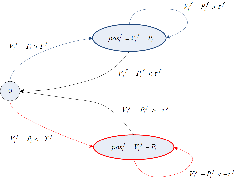
The positions of fundamentalist traders are proportional to the difference of actual price \(P_t\) to perceived fundamental value \(Vf_t\). However, an agent only enters a position when the different between price and value is above a given threshold, \(Vf_t - P_t | > Tf\). In that case, the position is determined as[3]:
| $$pos_t\,f = Vf_t - P_t\text{.}$$ | (3) |
Let’s note that when the price lies above the fundamental value, the asset is overpriced and the agent decides to sell; when the price lies below the fundamental value, then the agent decides to buy.
Fundamentalist investors keep their positions open until the price and the fundamental value converge, that is, until their difference is smaller than a given threshold. In that case, the agents liquidate their position:
| $$\begin{split} \text{If} \quad pos_{t-1}\,f > 0 \quad \& \quad Vf_t - P_t < \tau f \quad & \text{ then } \quad pos_t\,f = 0\text{.} \\ \text{If} \quad pos_{t-1}\,f < 0 \quad \& \quad Vf_t - P_t > -\tau f \quad & \text{ then } \quad pos_t\,f = 0\text{.} \end{split}$$ | (4) |
In case an agent has an open position, but the liquidation condition is not satisfied, then it simply updates its position based on the difference between price and value: if this difference has reduced (widened) since the position was opened, then the investors also reduces (increments) its position:
| $$pos_t\,f = Vf_t - P_t\text{.}$$ | (5) |
Fundamentalist investors are heterogeneous in their entry and exit thresholds
| $$Tf ~ U(T_{\min}, T_{\max})\text{,}\quad \tau f ~ U(\tau_{\min}, \tau_{\max})\text{.}$$ |
Once determined the new position, the agent calculates the order to be sent to the market-maker:
| $$\theta_t\,f = pos_t\,f - pos_{t-1}\,f\text{.}$$ | (6) |
Figure 1 summarises how the fundamentalist strategy works:
Technical traders (TREND)
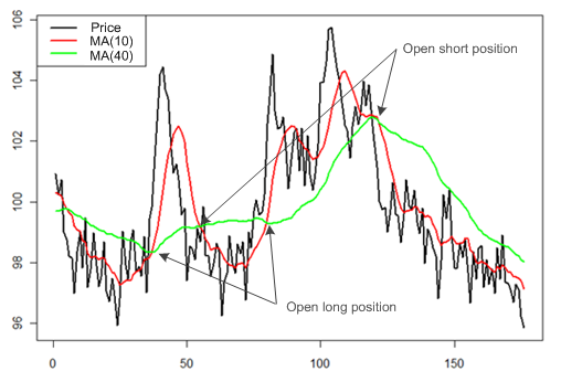
Technical traders exploit price trends, and for that aim we have implemented two of the most common techniques in real markets (Taylor 2005): to detect the start of a trend in prices, agents compare a short- and a long-term moving average of past prices; to detect the end of a price trend, agents rely on the technique of channel breakouts. To implement these rules, we have built on the practitioner literature, mainly on the description provided in (Kestner 2003).
At each time step, technical investors calculate two simple moving averages (MA) of past prices: one short-term MA that responds quickly to recent price movements, and a long-term MA that responds more slowly. Let \(w_S^{tr}\) and \(w_L^{tr}\) be the windows used by the technical agent \(tr\) to calculate his short- and long-term moving averages, respectively. The moving averages are then given by:
| $$\begin{split} MA(w_S^{tr})_t =& \frac{1}{w_S^{tr}} \cdot \sum_{i = t - w_S^{tr} + 1}^t P_i \\ MA(w_L^{tr})_t =& \frac{1}{w_L^{tr}} \cdot \sum_{i = t - w_L^{tr} + 1}^t P_i \end{split}$$ | (7) |
When the two moving averages cross, it is the key time to buy or sell: if the short-term MA crosses the long-term MA from below, the agent interprets it as the beginning of an upward trend and opens a long position; if the short-term MA crosses the long-term MA from above, the agent interprets it as the start of a downward trend and opens a short position (Figure 2).
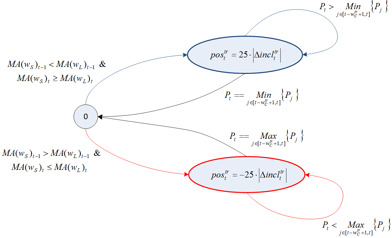
When the MA’s cross and the agent opens a position, it is proportional to the difference in slope between the two moving averages, because it is assumed that the greater this difference, the steeper the upward or downward price trend. Equations 8 and 9 specify the formula used by technical investors to calculate their position:
- If \(MA(w_S^{tr})_t\) crosses \(MA(w_L^{tr})_t\) from below, then the agent opens a long position:
- If \(MA(w_S^{tr})_t\) crosses \(MA(w_L^{tr})_t\) from above, then the agent opens a short position:
| $$pos_t^{tr} = 25 \cdot |\Delta incl_T^{tr}|$$ | (8) |
| $$pos_t^{tr} = -25 \cdot |\Delta incl_t^{tr}|\text{,}$$ | (9) |
- 25 is a normalisation factor aimed at having the same order of magnitude in the orders from fundamentalist and technical agents.
- \Delta incl_t^{tr}\) is the difference between the slope of the two MA’s: \(\Delta incl_t^{tr} = \arctan(MA(w_S^{tr})_t - MA(w_S^{tr})_{t-1}) -\arctan(MA(w_L^{tr})_t - MA(w_L^{tr})_{t-1})\)
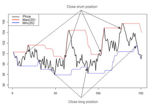
Technical investors keep their positions open until they think that the price trend has begun to reverse. In order to detect a trend reversal, the agents use a channel breakout rule: if the current price is the lowest in the last \(w_C^{tr}\) days, then the technical trader interprets that the price is going down, and any long position should be liquidated; if the current price is the highest in the last \(w_C^{tr}\) days, then the technical trader interprets that the price is going up, and any short position should be liquidated.
| $$\begin{split} \text{If}\quad \textit{pos}_{t-1}^{tr} > 0 \quad \& \quad P_t & == \textit{Min}_{j \in [t - w_C^{tr} +1, t]} \{P_j\}\quad \text{then}\quad \textit{pos}_t^{tr}=0\text{.}\\ \text{If}\quad \textit{pos}_{t-1}^{tr} < 0 \quad \& \quad P_t & == \textit{Max}_{j \in [t - w_C^{tr} +1, t]} \{P_j\}\quad \text{then}\quad \textit{pos}_t^{tr}=0\text{.} \end{split}$$ | (10) |
Note that when drawing the minimum and the maximum of the price over a period, a channel appears, which is why the method is called “channel breakout” (Figure 3).
As happens with the fundamentalist investors, when a technical agent has an open position, but the channel breakout conditions is not satisfied, then he simply updates his position keeping the same sign:
| $$\begin{split} \text{If}\quad \textit{pos}_{t-1}^{tr} > 0 \quad \text{then}\quad \textit{pos}_t^{tr}= 25 \cdot |\Delta incl_t^{tr}| \text{.}\\ \text{If}\quad \textit{pos}_{t-1}^{tr} < 0 \quad \text{then}\quad \textit{pos}_t^{tr}= -25 \cdot |\Delta incl_t^{tr}| \text{.}\\ \end{split}$$ | (11) |
Technical investors are heterogeneous in the windows of the moving averages and breakout channel
| $$w_S^{tr} \sim U(w_{S \min}^{tr}, w_{S \max}^{tr})\text{,}\quad w_L^{tr} \sim U(w_{L \min}^{tr}, w_{L \max}^{tr})\quad w_C^{tr} \sim U(w_{C \min}^{tr}, w_{C \max}^{tr})\text{.}$$ |
Once set the new position, the agent calculates the order to be sent to the market-maker:
| $$\theta_t^{tr} = pos_t^{tr} - \textit{pos}_{t-1}^{tr}\text{.}$$ | (12) |
Figure 4 summarises how the technical strategy works.
Value-at-risk model
Up to this point, we have assumed that agents exclusively relied on valuation models to determine the number of shares to buy or sell in any given time step. To account for the market risk of the portfolio, we now introduce a risk model based on VaR position limits. We assume that for a given portfolio and time horizon \\Delta t_h = t_h – t\) the variation of the portfolio value is distributed normally with mean \((mu = 0\) and normalised variance \(\sigma_t^2\). An estimate for the maximum loss of the portfolio value \(\textit{Value}^P\) for the confidence level \(\alpha\) is
| $$\textit{VaR}_t = z_{1-\alpha} \cdot \cdot \textit{Value}_t^P \cdot \sqrt{\Delta t_h}\text{,}$$ | (13) |
Let \(\theta_t\) be the order that an investor wants to issue according to its fundamentalist or technical strategy. Before sending this order to the market maker, the agent calculates the 1-tick VaR of the position it would have in the stock if the order \(\theta_t\) became effective:
| $$\textit{VaR}_t = z_{1-\alpha} \cdot \sigma_t \cdot |\textit{pos}_{t-1} + \theta_t| \cdot P_t\text{.}$$ | (14) |
In case the VaR of the desired position (Equation 13) does not exceeds the VaR limit LVaR of the agent, the order is sent to the market maker to calculate the new price; otherwise, the agent needs to reduce the order to a level where the VaR of the resulting portfolio is below the limit (LVaR):
| $$\textit{pos}_t^{\textit{red}} = (\textit{pos}_{t-1} + \theta_t)\cdot \frac{LVaR}{VaR_t}\text{.}$$ | (15) |
Then the order actually sent to the market maker needs to be adjusted:
| $$\theta_t^{\textit{red}} = \textit{pos}_t^{\textit{red}} - \textit{pos}_{t-1}\text{.}$$ | (16) |
Traders are heterogeneous in ther VaR limit and in the window used to calculate the volatility of the assets:
| $$\textit{LVaR} \sim U(\textit{LVaR}_{\min}, \textit{LVaR}_{\max})\text{,}\quad w^{\sigma} \sim U(w^{\sigma}_{\min}, Uw^{\sigma}_{\max})\text{.}$$ |
Measuring financial instability
The objective of this paper is to analyse whether countercyclical regulations contribute to market stability. It is difficult to define what financial stability exactly is, but all the proposed definitions agree that financial stability is linked to the absence of crises, stress or excessive volatility (Gadanecz & Jayaram 2008). It is even more difficult to measure financial stability: to this aim, central banks and other regulators use indices that combine simple indicators that provide information not only on financial markets but also on real economy or corporate sector to account for the fact that financial stability is connected to the proper functioning of the macroeconomic environment (Manamperi 2015)[4]. Our model is just a stylised version of a stock market, and so we cannot implement stability indicators pertaining to any sector other than financial markets. Building on the real-world indicators used by regulators in this sector, we will implement the following indicators of financial instability, which essentially measure the intensity of price movements and the fragility of market participants:
- Return volatility: Market volatility, which measures the size of price movements (Gadanecz & Jayaram 2008), is the most usual indicator of financial stability (The World Bank 2013). We define volatility as the standard deviation of the return series of an asset, \(r\), calculated within a window \(w\):
where \(\mu^r\) is the average of returns \(r\) calculated within the same window \(w\).$$\sigma_t^r = \sqrt{\frac{1}{w-1} \cdot \sum_{k = t-w+1}^t (r_k - \mu_t^r)^2 }\text{,}$$ (17) - Return kurtosis[5]: Kurtosis of returns is the fourth central moment of the return distribution:
- Hill tail index: Apart from kurtosis, the behaviour of the tails of the return distribution can be described through the tail index. In recent years it has been determined that the complementary cumulative distribution function of returns asymptotically follows a power law distribution (also sometimes called Pareto distribution)[6]
and so the descent of the probability density function also follows a power law distribution in the tails with exponent \(\alpha+1\) (Cristelli 2014). The exponent \(\alpha\) coincides with the so-called tail index of the return distribution, which measures the order of the largest absolute moment that is finite (for example, the tail index of a normal distribution is \(\infty\) because all of its moments are finite, and the greater this index is, the thinner the distribution tails are) (Cont 2001). The exponent \(\alpha\) is usually estimated with the Hill index[7], which is the maximum-likelihood estimator of the tail index (Einarsson 2013). So, when the Hill index of the return series takes a low value, it indicates that returns are more likely to take extreme values, what is a sign of heightened instability (Hermsen 2010).$$F(x) = P(X>x) \sim x^{-\alpha}$$ - Investor strength: Building on the z-score used to measure the fragility of banks (Beck et al. 2011), we define an indicator of investor strength as the ratio between the end-of-simulation accumulated profits and the standard deviation of these final profits. This indicator provides an idea of the consistency of traders’ results and so of their stability.
| $$k_T^r = \frac{\frac{1}{w} \cdot \sum_{k = t-w+1}^t (r_k - \mu_t^r)^4}{(\sigma_t^r)^4}\text{,}$$ | (18) |
Parameters
Table 1 summarises the value of all the model parameters used in the results described next. When choosing these values, we have applied the following criteria:
- For those parameters that are a direct adaptation of real strategy parameters, we have simply chosen realistic values.
- For those parameters not ‘observable’ in real markets, we have adjusted their value with the aim of obtaining reasonable price dynamics that satisfy as much as possible the stylised facts of stock markets (Cont 2001; Taylor 2005). In particular, the model captures the following properties:
- Lack of return autocorrelation: The autocorrelation function of the return series obtained from the simulations tend to 0 when the lag increases.
- Fat tails: The distribution of the return series obtained from the model is more leptokurtic than the normal distribution. Returns present excess kurtosis, and their histogram has more mass in the center and the tails than a normal distribution.
- Volatility clustering: The autocorrelation function of volatility –estimated either as the absolute value or the square of returns – remains positive for several lags, and volatility presents long-term memory.
- Correlation between volume and volatility: The correlation between trading volume (calculated as the sum of orders issued by all the agents in absolute value) and volatility is positive.
- Volume autocorrelation: The autocorrelation function of the volume series obtained from simulations remains positive for several lags and decays slowly to 0, and volume has long-term memory.
Next, we describe in more detail how we have calibrated each parameter[8]:
- Parameters associated to price formation: The impact of traders in price formation is normalised with the liquidity parameter \(\lambda\), so this parameter is linked to the number of agents (the higher the trader population size, the higher the liquidity). Although this parameter has an empirical interpretation, its value is not observable, and it has then been calibrated by looking at the stylised facts replicated by the model. The random term in price formation (see Formula 1) is governed by the standard deviation parameter \(\sigma_P\), whose value has been set to obtain an overall price volatility value in line with empirical daily volatility of S&P500 (assuming here that one time step is equivalent to one trading day).
- Parameters associated to fundamental value formation: The fundamental value process depends on the standard deviation term \(\sigma_V\). This has been calibrated based on the stylised facts replicated by the model.
- Parameters associated to the fundamentalist strategy: Although we do not have empirical evidence on which thresholds are used by fundamentalist traders, we have used plausible values for the mispricing level required to enter and exit a position (\(T^f, \tau^f\)), and we have fine-tuned these values – together with the unobservable parameter \(v^f\) – by looking at the stylised facts replicated by the model.
- Parameters associated to the technical strategy: To implement the technical trading strategy, we have built on techniques widely used in real markets, and so when it came to setting the values of the different windows we turned to the practitioner literature. The windows for the short- and long-term moving averages (\(w_S^{tr}, w_L^{tr}\)) move around 10 and 40 as these are the values usually employed by real technical investors (Kestner 2003); the window for the exit channel moves around 20 as this is the typical period (Milton 2016).
| Parameter | Value | Parameter description |
| \(N_{\textit{ticks}}\) | 4000 | Number of ticks of each run |
| \(\lambda\) | 400 | Liquidity |
| \(P_0\) | 100 | Initial price |
| \(\sigma_P\) | 0.4 | Standard deviation for random term in price formation |
| \(N_{\textit{FUND}}\) | 200 | Number of fundamentalist traders |
| \(N_{\textit{TREND}}\) | 200 | Number of technical traders |
| \(\sigma_V\) | 0.25 | Standard deviation for random term in fundamental value formation |
| \([v_{\min}, v_{\max}\) | [-8, 8] | Boundaries of the uniform distribution that sets the difference between the fundamental value and the value perceived by each fundamentalist trader |
| \([T_{\min}, T_{\max}]\) | [2, 5] | Boundaries of the uniform distribution that sets the entry thresholds of fundamentalist traders |
| \([\tau_{\min}, \tau_{\max}]\) | [-0.5, 1] | Boundaries of the uniform distribution that sets the exit thresholds of fundamentalist traders |
| \([w_{S \min}^{tr}, w_{S \max}^{tr}]\) | [5, 15] | Boundaries of the uniform distribution that sets the window of short-term moving average used by technical traders |
| \([w_{L \min}^{tr}, w_{L \max}^{tr}]\) | [35, 50] | Boundaries of the uniform distribution that sets the window of long-term moving average used by technical traders |
| \([w_{C \min}^{tr}, w_{C \max}^{tr}\) | [5, 30] | Boundaries of the uniform distribution that sets the window of exit channel used by technical traders |
| \(\alpha\) | 99% | Confidence level |
| \([\textit{LVaR}_{\min}, \textit{LVaR}_{\max}]\) | Variable | Boundaries of the uniform distribution that sets the VaR limit of each agent |
| \([w_{\min}^{\sigma}, w_{\max}^{\sigma}]\) | Variable | Boundaries of the uniform distribution that sets the window used to calculate the stock volatility |
Effect of VaR models
In this section we will show that the use of VaR position limits impacts price dynamics and market stability[9]. For that aim, we will next study how an increasing use of VaR-based position limits has a noticeable effect on the instability indicators described in Section 2.30.
We consider a one-asset market where the proportion of traders – both fundamentalist and technical investors – that manage their risk with VaR limits rises across experiments from 0% to 100%. That is, in the first experiment no agent uses VaR, whereas in the last experiment all agents are using VaR. We assume that all traders are homogeneous in their VaR limit and volatility window:
| $$\begin{split} \textit{LVaR} &= 40 \\ w^{\sigma} &= 20 \end{split}$$ |
In all the experiments, simulations have a duration of 4000 time steps (in order to calibrate variables such as price volatility we assume that each time step is equivalent to 1 day, and so each run has an equivalent duration of 16 years). Each experiment consists of 250 runs and uses the parameters listed in Table 1. We are using identical random number sequences across the different experiments so that the results become comparable.
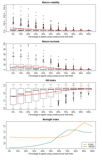
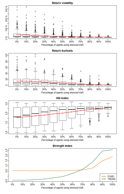
Figure 5 shows the evolution of the different instability indicators[10] when the percentage of traders using a VaR system increases from 0% to 100%. The four indicators show that the market becomes more unstable when most traders manage their risk with VaR limits: the volatility of returns heightens, the kurtosis of returns rises and their Hill tail index goes down – which indicates that extreme returns are more frequent –, and the index of trader strength also worsens – because the dispersion of agent profits increases. When a high percentage of traders are using VaR limits, the average market instability increases because of the emergence in some runs of a particular price dynamics which we have called ‘VaR cycles’. In fact, the outliers observed in Figure 5 are realised in those runs where VaR cycles are specially remarkable. Let’s have a look at a particular simulation to describe in detail the functioning of such cycles.
Evolution of instability indicators when the percentage of agents using VaR increases from 0% to 100%. From top to bottom: return volatility, return kurtosis, return Hill tail index, and agent strength index.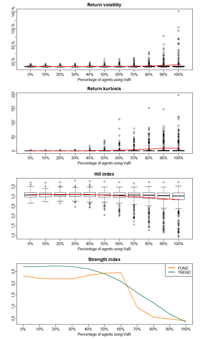
Description of a VaR cycle
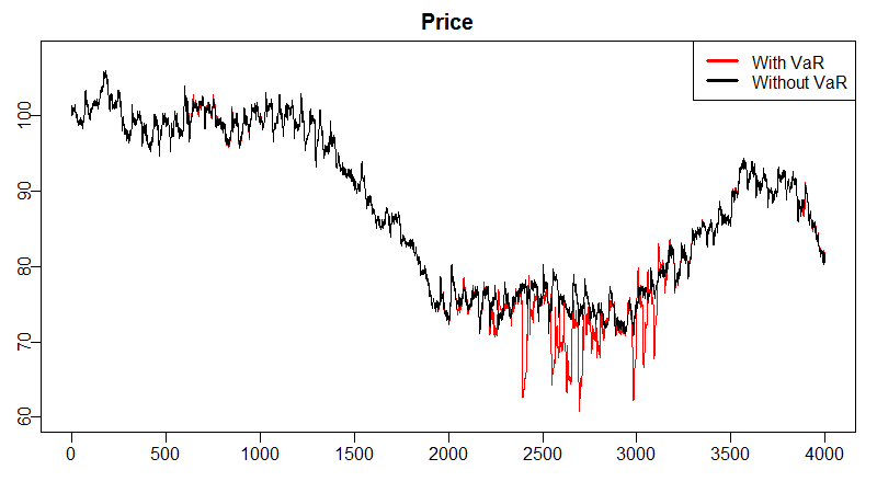
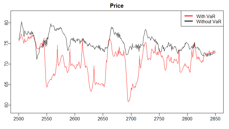
Figure 6 compares the price time series obtained in a particular simulation when (1) no agent uses VaR limits (in black), and (2) when all the agents use a VaR model with a limit LVaR = 40 and a volatility window \(w^{\sigma} = 20\) = 20 (in red). A different behaviour can be appreciated from \(t = 2400\) onwards. For better clarity, a zoom of the price series for \(t = 2500\dots 2850\) is provided in Figure 7 to appreciate the differences in price dynamics.
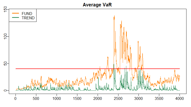
Price behaviour from \(t = 2400\) on is due to the trader action after reaching their VaR limit. Figure 8 exhibits the VaR of agents’ portfolio, averaged over fundamentalist and technical investors. This VaR is calculated with the positions that agents would accumulate if they were allowed in the current time step to buy or sell the amount dictated by their trading strategy. From \(t = 2400\) onwards, agents’ VaR exceeds their LVaR limit – represented with a horizontal, red line –, and so traders are forced to forget about their ‘desired’ orders and need to reduce their portfolio to keep their VaR below the limit.
Note that major price movements are caused by agents reducing their portfolio, but this does not mean that price exhibits VaR cycles every time that an agent is forced to liquidate part of its positions. In fact, there are some fundamentalist agents that touch their VaR limit before \(t = 2400\) and are thus forced to reduce their positions, but the average VaR over all the fundamentalist population lies below the limit as seen in Figure 8. As these reductions are small compared to the total trading volume, their impact on price is minor. However, when most agents accumulate substantial positions and their portfolio VaR is close to the limit, any small upsurge in volatility can make VaR rise above the limit and force traders to liquidate positions. When a number of traders must reduce their portfolio at the same time, these reductions have a noticeable impact on the price and, in turn, on volatility.
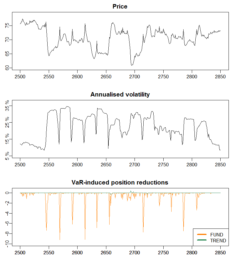
Figure 9 shows the time series of price, return volatility and ‘forced’ portfolio reductions of fundamentalist (in orange) and technical traders (in green). When these reductions are different from zero, it indicates that at least some agents not only cannot send to the market their ‘desired’ order – that is, the order dictated by their trading strategy –, but are forced to partially liquidate their positions to reduce their VaR to an acceptable level. It can be observed that within the interval \(t = 2500-2850\) – zoomed in Figure 10 –, the first substantial portfolio reductions around \(t = 2550\) push the price down and the volatility up, but this process keeps along for a while because the increase in volatility rises again the VaR of agents, which must reduce again their positions, and so on.
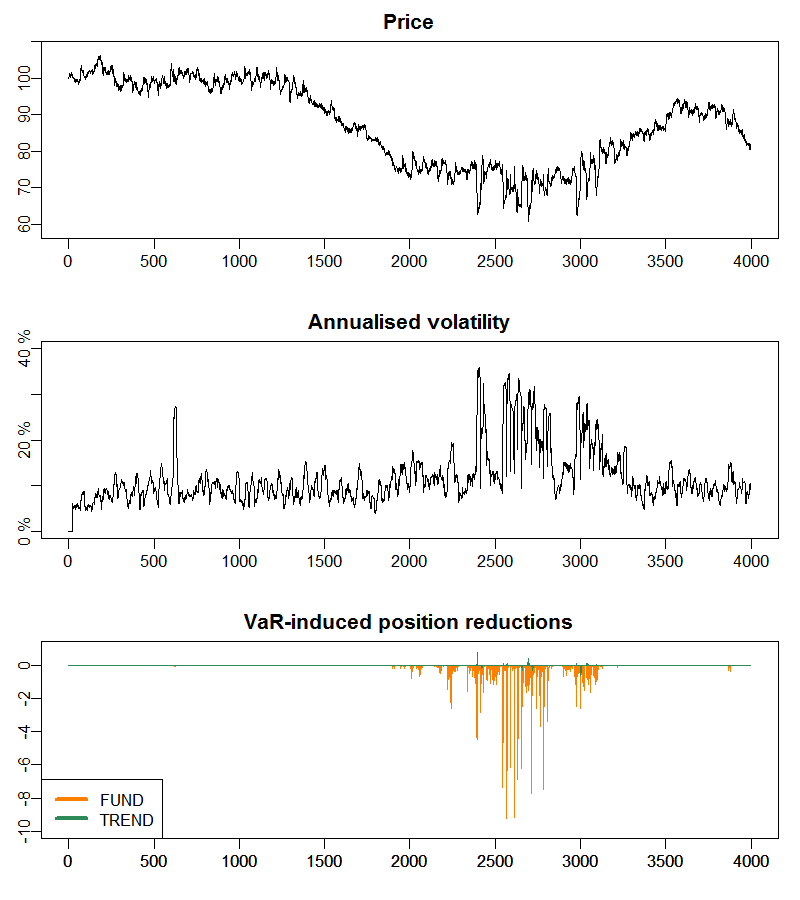
When agents have sufficiently reduced their portfolio, their orders get smaller and the price decline slows down. Volatility remains high while the window over which it is calculated still includes the first major movements in price. Nevertheless, when time goes by and volatility decreases, traders start trading again as usual. If there is some coordination between investors and they simultaneously buy or sell, then the price movements can be substantial enough to raise again volatility and cause agents to reach their VaR limit. The ‘VaR cycle’ may thus repeat once more (see for example the portfolio reductions around \(t = 2570, 2590\), etc. which plunge the price and raise the volatility).
In the experiments just described we have seen that the higher the proportion of agents using VaR, the higher the possibility that VaR cycles emerge, that is, episodes where the reduction of positions by some traders rises the volatility enough to force other agents to sell off part of their holdings to reduce their exposure, thereby increasing volatility again and reinforcing the destabilisation spiral. Given that the market is more likely to suffer instability bouts when all of the agents use a VaR system, our experiments suggest that, at the global level, it would be more beneficial that not all of the investors control their positions with a VaR-based limit; they could use other types of risk management models, or at least they could use more flexible limits that do not force them to reduce their portfolio automatically when exceeding their risk threshold.
The appearance of VaR cycles largely depends on the value of the parameters used by traders in their VaR model. We will next summarise the effect of the volatility window and the VaR limit in the potential market destabilisation.
Effect of VaR model parameters
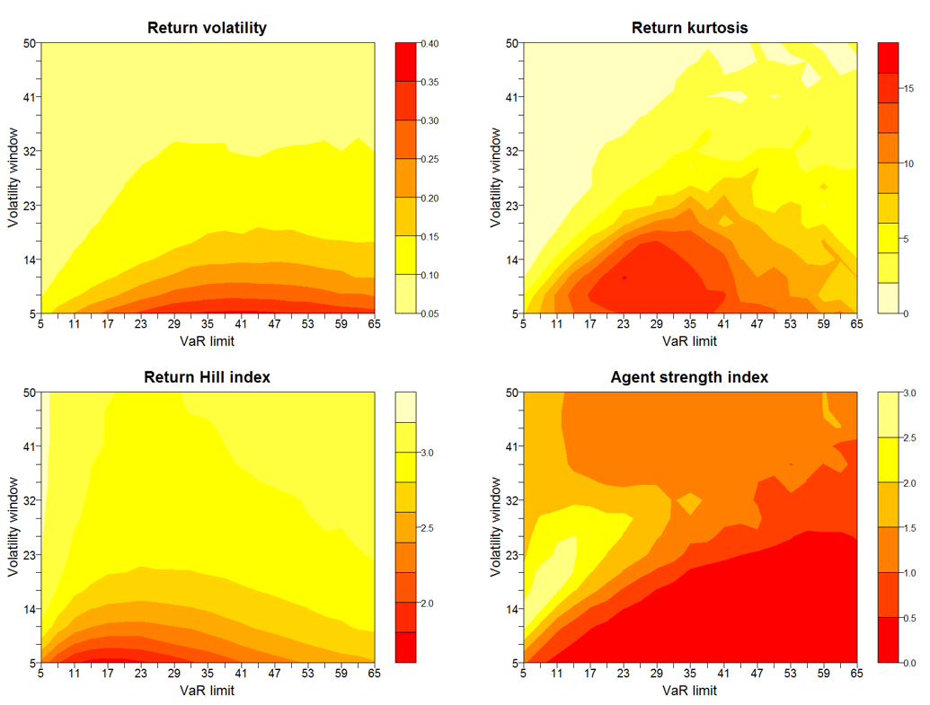
We will explore next the impact of a varying value of the window used to calculate volatility in the VaR model, \(w^{\sigma}\), and of the position limit used by the agents to control the risk of their portfolio, LVaR. We summarise in Figure 11 the behaviour of the different instability indicators when the VaR limit takes values from \(\textit{LVaR} = 5\) to \(\textit{LVaR} = 65\)[11] and the window volatility takes values from \(w^{\sigma} = 5\) to \(w^{\sigma} = 50\)[12] days. In all the contour plots the colour red identifies the most unstable situation (for example, the highest values of volatility or the lowest values of the Hill index).
Several indicators point out that the most unstable scenario is achieved when investors use a small window to calculate volatility and they moreover use an intermediate VaR limit; return volatility and Hill index are particularly clear in this regard. On the one hand, when volatility is calculated using a small window, that is, considering just a few observations, each of these observations has a great weight in the outcome, and volatility turns out to be very sensitive to recent price movements. So when the volatility window is small, VaR can significantly increase from one tick to the next, whereas when volatility is calculated with a higher window, a much sharper price variation is required for volatility to notice it. For this reason, using a medium- or long-term window to calculate volatility highly reduces the appearance of VaR cycles and so improves market stability.
On the other hand, the behavior of the various indicators leads us to conclude that the market is particularly stable when the limits are either very restrictive or very loose. If the VaR limit takes a low value, this considerably constrains the positions that agents can take, because the VaR of their portfolio is proportional to the asset positions. So, even though they reach their limit more frequently and are forced to reduce their portfolio, they cannot send large orders to the market because their positions are not huge, and VaR-caused reductions have a smaller effect in market dynamics. On the other hand, if the VaR limit takes a high value, then agents are less likely to reach their limit, and so price dynamics do not differ much from the case in which agents do not manage their risk (in fact, a scenario with a high enough VaR limit is equivalent to a model without VaR). It is for intermediate values of the VaR that prices show the most interesting dynamics, with the appearance of VaR cycles when the risk-driven portfolio reductions have a noticeable effect on prices and volatility. We note that there is no need to consider unrealistic values of the VaR limit for instability episodes to appear: VaR cycles are most likely to appear for \(\textit{LVaR} = 11\text{--}14\), which correspond approximately to 11% -45% of the average value of traders’ portfolio, and in real markets it is quite probable that a financial institution facing losses of this magnitude liquidates some positions to prevent that losses heighten.
Can regulation counteract the effects of VaR models?
In Section 3 we have seen that the widespread use of VaR system has the potential to generate instability spirals where agents are forced to reduce their portfolios when hitting their VaR limit, and these reductions move the prices, increase market volatility and cause a new wave of reductions that reinforce market instability. In view of the procyclicality induced by this type of risk management models, whose use in particular is encouraged by the Basel regulatory capital framework, the new Basel III Capital Accord introduces two measures aimed at reducing the procyclicality of capital requirements: a countercyclical buffer that urges banks to increase their capital reserves during “good times” and reduces capital requirements when the situation worsens, and stressed VaR, which adds an additional term to the calculation of market risk requirements that covers a period of special financial turmoil.
In this section we will study the effectiveness of two regulations that build on the two countercyclical measures introduced in Basel III: countercyclical VaR limits – based on the countercyclical buffer (Sections 4.4-4.8), – and stressed VaR (Sections 4.9-4.15). To put to test both measures, we consider precisely the model configuration where most indicators have shown that the use of VaR induces a greater level of instability. In Section 3 we have seen that it is more likely that VaR cycles emerge for intermediate values of the VaR limit and for a small volatility window. For this reason, in the experiments described below we choose the following values of the VaR model parameters:
| $$\begin{split} \textit{LVaR}_{\min} &= 30\text{,}\quad \textit{LVaR}_{\max} = 40\\ w^{\sigma}_{\min} &= w^{\sigma}_{\max} = 5 \end{split}$$ |
In this ‘adverse’ scenario we will better see if the proposed regulations are successful in stabilising the market, and which one is more effective in this regard.
Countercyclical VaR limits
The principal objective of the Basel III countercyclical buffer is to avoid the natural inclination for banks to relax their risk control standards during periods of credit growth by urging them to increase their capital requirements. In downturns, these requirements are reduced so that credit supply is not constrained and economy performance is not impaired (McCoy 2015). The adjustment of the countercyclical buffer depends on the macroeconomic conditions in which banks operate, and follows a rule-based approach combined with discretionary judgement by national policymakers (Basel Committee on Banking Supervision 2017). As our model does not consider the macroeconomic sector and cannot account for the discretion attributed to regulators, we cannot implement the countercyclical buffer as it stands in the Basel III Accord; instead, we will model a rule-based regulatory mechanism that captures its essence and primary objective: countercyclical VaR limits.
We next consider a variation of the model presented in Section 2 where VaR limits are variable and are adjusted according to the financial situation, using the same rationale behind the countercyclical buffer: when the market is stable, VaR limits are reduced to prevent agents from accumulating excessive positions. When, on the contrary, the market is unstable, VaR limits are risen to avoid that agents are forced to liquidate their positions and exacerbate instability. To decide when the market is (or not) stable, agents compare the current volatility to the historical volatility, and update their VaR limit according to the ratio between both volatility values:
| $$\textit{LVaR}_t = \textit{LVaR}_0 \cdot \frac{\sigma_t}{\bar{\sigma}_t}$$ | (19) |
To test the effect of this regulatory measure, we consider a market where the proportion of agents that use countercyclical VaR limits rises across experiments from 0% to 100%. That is, in the first experiment no agent uses countercyclical VaR limits, whereas in the last experiment all agents are using them. As said above, we assume that all traders are managing their risk with VaR using those values for the (initial) VaR limit and volatility window which maximise market instability[13].
Figure 12 shows the evolution of the different instability indicators[14] when the percentage of traders using countercyclical VaR limits increases from 0% to 100%. The four indicators show that market stability improves when more and more traders use countercyclical limits to manage their risk: the volatility of returns declines, the kurtosis of returns goes down and their Hill tail index increases – which indicates that extreme returns are less frequent –, and the index of trader strength also rises – because there is less dispersion in agent profits. In fact, it is sufficient that half the population uses this regulatory measure to observe a noticeable recovery in instability indicators, because the pressure to liquidate positions gets smaller and so VaR cycles are less likely to appear.
Further to the results shown in Figure 12, we have conducted a series of Wilcoxon–Mann–Whitney tests[15] to compare the mean instability of the market – measured as the return volatility – under different percentages of agents using countercyclical VaR limits. Two-sided p-values obtained from each test are shown in Table 2, where the percentages shown in row and column headers indicate the percentage of agents using countercyclical VaR limits in the two scenarios being compared. We can observe that there is no significant difference in return volatility when the percentage of agents using countercyclical Var limits is similar (cells close to the diagonal of the table); however, an increase of only 20% in this percentage can produce a noticeable effect on price dynamics that leads us to reject the null hypothesis and conclude that volatility is significantly different –in Table 2 we have highlighted in yellow and orange those tests where the null hypothesis is rejected at a significance level of 0.05 and 0.01, respectively.
| Percentage of agents using countercyclical VaR limits | |||||||||||
| 0% | 10% | 20% | 30% | 40% | 50% | 60% | 70% | 80% | 90% | 100% | |
| 0% | 0.26 | <0.05 | <0.01 | <0.01 | <0.01 | <0.01 | <0.01 | <0.01 | <0.01 | <0.01 | |
| 10% | 0.26 | 0.20 | <0.01 | <0.01 | <0.01 | <0.01 | <0.01 | <0.01 | <0.01 | <0.01 | |
| 20% | <0.05 | 0.20 | 0.17 | <0.01 | <0.01 | <0.01 | <0.01 | <0.01 | <0.01 | <0.01 | |
| 30% | <0.01 | <0.01 | 0.17 | 0.17 | <0.01 | <0.01 | <0.01 | <0.01 | <0.01 | <0.01 | |
| 40% | <0.01 | <0.01 | <0.01 | 0.17 | NULL | <0.05 | <0.01 | <0.01 | <0.01 | <0.01 | <0.01 |
| 50% | <0.01 | <0.01 | <0.01 | <0.01 | <0.05 | 0.12 | <0.01 | <0.01 | <0.01 | <0.01 | |
| 60% | <0.01 | <0.01 | <0.01 | <0.01 | <0.01 | 0.12 | 0.11 | <0.01 | <0.01 | <0.01 | |
| 70% | <0.01 | <0.01 | <0.01 | <0.01 | <0.01 | <0.01 | 0.11 | NULL | 0.23 | 0.09 | 0.12 |
| 80% | <0.01 | <0.01 | <0.01 | <0.01 | <0.01 | <0.01 | <0.01 | 0.23 | 0.65 | 0.79 | |
| 90% | <0.01 | <0.01 | <0.01 | <0.01 | <0.01 | <0.01 | <0.01 | 0.09 | 0.65 | 0.84 | |
| 100% | <0.01 | <0.01 | <0.01 | <0.01 | <0.01 | <0.01 | <0.01 | 0.12 | 0.79 | 0.84 |
Stressed VaR
In addition to the countercyclical buffer, Basel III Accord introduces the stressed VaR to reduce the specific procyclicality caused by market risk requirements. The stressed VaR component is calculated as the VaR of the current portfolio during a period of significant stress (Basel Committee on Banking Supervision 2010). It provides then an estimation of the maximum loss that the current portfolio could suffer in the case of an extreme event.
Stressed VaR is calculated using the same methodology than the usual VaR with the only difference that instead of building on recent volatility data it builds on historical volatility data belonging to a period of financial stress, such as the crisis of 2007-08 when banks suffered significant losses (Basel Committee on Banking Supervision 2010). Market risk capital requirements are then calculated as the sum of the usual VaR plus the stressed VaR. This additional term increases the capital reserves to be held by banks and this is expected to have a positive impact on market resilience.
To analyse the effectiveness of this measure, we will add a stressed VaR component to the risk management system employed by the agents. Building on the specifications of Basel III Accord (Basel Committee on Banking Supervision 2010), we calculate the stressed VaR (sVaR) as the usual VaR, but taking the most volatile period since the start of the simulation to compute volatility. That is, we calculate stressed VaR following Equation 13 but replacing current value of volatility \\sigma_t\) by its highest value since the start of the simulation. The total VaR of the portfolio is then the sum of the usual VaR plus the stressed VaR, and agents must ensure at each time step that this total VaR does not exceed their VaR limit LVaR.
To test the effect of this regulatory measure, we consider a market where the proportion of agents that use stressed VaR rises across experiments from 0% to 100%. As done in the experiments with countercyclical VaR limits, we assume that all traders are managing their risk with VaR using those values for the VaR limit and volatility window which maximise market instability[16].
Figure 13 shows the evolution of the different instability indicators[17] when the percentage of traders using stressed VaR increases from 0% to 100%. The four indicators show that market stability improves when more and more traders add the stressed VaR component to their usual VaR. These results are qualitatively similar to those obtained for the case of countercyclical VaR limits, and as observed in Sections 4.4-4.8, it is sufficient that half the population uses this regulatory measure to observe a noticeable recovery in instability indicators. In this case, the need to keep total VaR below the limit restricts agents’ capacity for action and reduces the number of VaR cycles.
When agents use stressed VaR, the total VaR of the portfolio increases because the additional term of stressed VaR must be taken into account. In a sense, this has an effect similar to lowering the VaR limit, as agents must make a harder effort to keep their positions at bay: if they accumulate higher positions, not only their usual VaR increases, but also their stressed VaR, and in this situation it is easier to exceed the VaR limit and be forced to liquidate positions. This constrains agents’ positions, reduces their orders and – when the VaR limit is hit – moderates the impact of their portfolio reductions on price. On the other hand, the additional term of stressed VaR is more ‘constant’ than the usual VaR since it is calculated on the basis of the most volatile period and so it is less likely to react to current volatility (unless it is a specially unstable moment). In this way the use of stressed VaR decreases the emergence of VaR cycles and helps to stabilise the market.
As done in Sections 4.4-4.8, we have also conducted a series of Wilcoxon–Mann–Whitney tests to compare the instability of the market under different percentages of agents using stressed VaR. The results, summarised in Table 3, exhibit a similar pattern: the null hypothesis gets rejected when slightly moving away from the table diagonal, meaning that a small increase in the percentage of agents using stressed VaR tends to be sufficient to produce a significant reduction in market volatility.
| Percentage of agents using stressed VaR | |||||||||||
| 0% | 10% | 20% | 30% | 40% | 50% | 60% | 70% | 80% | 90% | 100% | |
| 0% | 0.20 | <0.01 | <0.01 | <0.01 | <0.01 | <0.01 | <0.01 | <0.01 | <0.01 | <0.01 | |
| 10% | 0.20 | 0.14 | <0.01 | <0.01 | <0.01 | <0.01 | <0.01 | <0.01 | <0.01 | <0.01 | |
| 20% | <0.01 | 0.14 | 0.19 | <0.01 | <0.01 | <0.01 | <0.01 | <0.01 | <0.01 | <0.01 | |
| 30% | <0.01 | <0.01 | 0.19 | 0.09 | <0.01 | <0.01 | <0.01 | <0.01 | <0.01 | <0.01 | |
| 40% | <0.01 | <0.01 | <0.01 | 0.09 | 0.16 | <0.01 | <0.01 | <0.01 | <0.01 | <0.01 | |
| 50% | <0.01 | <0.01 | <0.01 | <0.01 | 0.16 | 0.07 | <0.01 | <0.01 | <0.01 | <0.01 | |
| 60% | <0.01 | <0.01 | <0.01 | <0.01 | <0.01 | 0.07 | 0.05 | <0.01 | <0.01 | <0.01 | |
| 70% | <0.01 | <0.01 | <0.01 | <0.01 | <0.01 | <0.01 | 0.05 | 0.12 | <0.01 | <0.01 | |
| 80% | <0.01 | <0.01 | <0.01 | <0.01 | <0.01 | <0.01 | <0.01 | 0.12 | 0.08 | <0.01 | |
| 90% | <0.01 | <0.01 | <0.01 | <0.01 | <0.01 | <0.01 | <0.01 | <0.01 | 0.08 | 0.38 | |
| 100% | <0.01 | <0.01 | <0.01 | <0.01 | <0.01 | <0.01 | <0.01 | <0.01 | <0.01 | 0.38 |
Comparative analysis of countercyclical regulations
In Sections 4.4-4.8 and 4.9-4.15 we have analysed two regulatory measures aimed at reducing the procyclicality of VaR systems: countercyclical VaR limits and stressed VaR. We have seen that both measures meet their objective: when put to test under the most adverse scenario, both reduce noticeably market instability. In fact, it is usually enough that half the population uses one of these measures for the instability indicators to show a clear improvement.
But which of the two measures is more effective? To answer this question, in Figure 14 we summarise in a comparative way the evolution of the different instability indicators when the proportion of traders that use countercyclical limits or stressed VaR increases from 0% to 100%. This will allow us to better discern if one of those two measures has a more palpable effect on counteracting the emergence of VaR cycles.
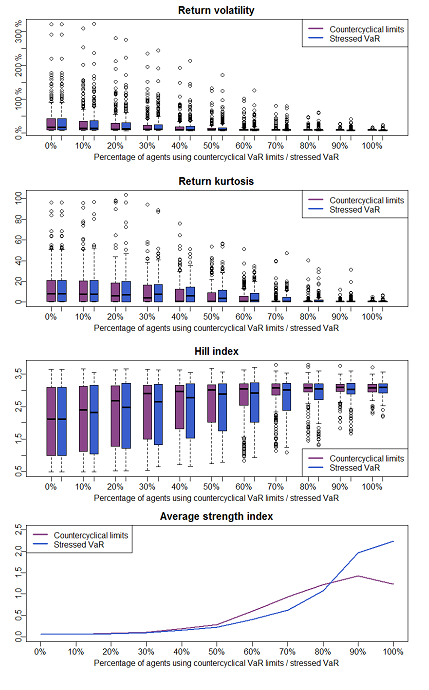
The various indicators reveal that the adoption of countercyclical VaR limits and stressed VaR has a similar effectiveness in neutralising the impact of VaR cycles and reduce market instability: all the indicators take comparable values when the proportion of agents that use one or the other regulatory measure increases, so it indicates that both countercyclical mechanisms are equally effective.
To test if there is a statistically significant difference between the effects of countercyclical VaR limits and stressed VaR, we have run a series of Wilcoxon–Mann–Whitney tests with null hypothesis that return volatility when x% of agents are using countercyclical VaR limits does not differ from when the same percentage of agents are using stressed VaR. P-values obtained from each test are shown in Figure 4, where we can observe that there is no significant difference in return volatility when the percentage of agents using countercyclical Var limits or stressed VaR is low to medium. Only when most agents are using one of these measures the null hypothesis is rejected and we then can conclude that the effect of the two regulations is sufficiently distinguishable from a statistical point of view.
| Percentage of agents using countercyclical Var limits or stressed VaR | ||||||||||
| 0% | 10% | 20% | 30% | 40% | 50% | 60% | 70% | 80% | 90% | 100% |
| 0.89 | 0.71 | 0.71 | 0.36 | 0.60 | 0.26 | 0.10 | <0.05 | <0.01 | <0.01 |
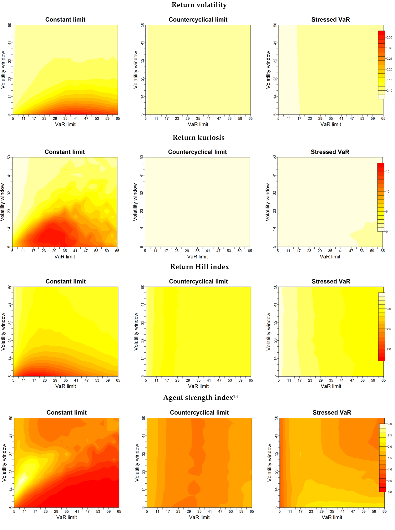
To complete the analysis we provide below in Figure 15 heatmaps of the different instability indicators that show their evolution for a wider range of the (initial) VaR limit (\(LVaR_0 = 5..65\)) and the volatility window (\(w_{\sigma} = 5..50\)). In the experiments run in Sections 4.4-4.8 and 4.9-4.15 we have focused on the combination of parameters for which the market is more likely to suffer VaR cycles, but the graphics in Figure 15 provide a broader perspective on the behaviour of the indicators for other values of the (initial) VaR limit and the volatility window.
To get a better idea of the effect of both regulatory measures, in Figure 15 we contrast the behaviour of the four instability indicators with the baseline scenario where all agents use VaR with constant VaR limits (that is, the case considered in section 3), to see whether countercyclical VaR limits and stressed VaR reduce market instability for any combination of the parameters LVaR and \(w_{\sigma}\), and to compare the extent of this reduction. In all the heatmaps the colour red identifies the most unstable situation (for example, the highest values of volatility or the lowest values of the Hill index), and to facilitate the comparative analysis, we use the same scale in each row. In this way the graphics in Figure 15 provide a good insight on which measure turns out to be more effective for a broader range of parameters.
Discussion
The comparative analysis in Figure 15 has clearly shown that both the use of countercyclical VaR limits and stressed VaR reduce market instability not only in the scenario most prone to the appearance of VaR cycles (as seen in Sections 4.4-4.8 and 4.9-4.15), but also for the rest of values of the VaR limit and the volatility window. As already observed in Section 4.16-4.21, the results obtained with countercyclical limits or stressed VaR appear to be equally effective, both in the “critical” region of highest instability (that is, the read areas in the left-hand graphics in Figure 15), and in the rest of scenarios.
We can conclude from this that the reformulation of capital requirements introduced in Basel III Accord, which introduces the countercyclical buffer and adds stressed VaR to usual VaR, is a wise decision to improve capital standards and strengthen bank stability because it prevents or reduces the severity of high-instability episodes. However, it must also be taken into account that these are strict measures, as they significantly increase capital requirements, especially in the case of stressed VaR. Countercyclical VaR limits vary according to market fluctuations and may leave more leeway to financial institutions during episodes of turmoil; however, the stressed VaR always refers to a historical period of significant stress and therefore its value exceeds that of usual VaR (and despite being less reactive to current volatility, it will tend to grow if instability increases).
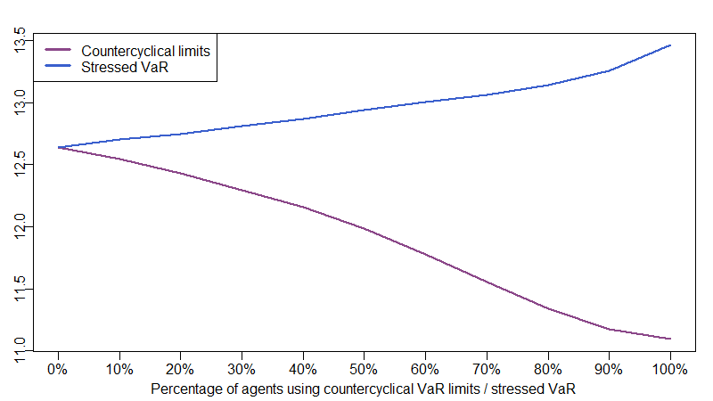
So stressed VaR improves market stability, but at the cost of constraining the freedom of action of traders, who cannot accumulate large positions. In fact, stressed VaR has been criticised by the banking industry for the significant increase in the capital reserves they need to keep (Choudhry 2013; Lobanov 2012). This has an impact not only at the individual level, but also at the global level, as market efficiency decreases. In Figure 16 we find that the average distance between the time series of price and fundamental value goes up when the number of agents that use stressed VaR increases, since the action of fundamentalist traders – who prevent price from diverging from fundamental value – gets constrained and their ability to move the price towards fundamental value diminishes. However, it is not the case when the proportion of agents that use countercyclical VaR limits increases. This highlights that, although stressed VaR is an effective measure against financial instability, it has side effects that cannot be ignored, and would provide support to those economists that advocate for the adoption of countercyclical buffers into the VaR model itself instead of the addition of the stressed VaR term (Choudhry 2013).
Conclusions
In recent times the use of risk management systems has become widespread, and VaR has come to be the main methodology at most financial institutions. VaR models assume that risk is exogenous, that is, prices are not affected by actions of financial institutions that are trying to estimate the risk of their portfolio (Morris & Shin 2000; Danielsson et al. 2001). This is possibly right most of the time, when investors trade with different strategies and criteria. But it is precisely those (even if very rare) occasions when investors act in a uniform way that are of interest, since traders’ aggregate action can move the prices and trigger an instability spiral. The use of VaR systems is precisely one of the mechanisms that contribute to homogenise the behaviour of market participants: when – for any reason – volatility goes up, so does the VaR of investors and in case it exceeds the limit, agents are forced to reduce their portfolio at the same time. If, in addition, traders hold similar positions, the way is paved for portfolio reductions to plunge the price, increase the volatility and raise again the traders’ VaR. It is therefore a scenario of endogenous risk, since the use of VaR systems has the potential to amplify market instability and feed it back.
In this article we have studied in which circumstances VaR systems do amplify price fluctuations, and have tested the effectiveness of two regulatory measures aimed at improving the resilience of financial markets. To this aim, we have built an agent-based model, which can capture both the effect that market has on individual investors as well as the global effect that emerges from the aggregation of individual actions. Indeed, the flexibility of agent-based models to reflect the behaviour of individual agents and their interactions makes them a more suitable approach for policy analysis than traditional, equilibrium-based models (Fagiolo & Roventini 2017).
We have considered a model of fundamentalist and technical traders which manage their risk with a simple VaR model and must reduce their positions when the risk of their portfolio goes above a given threshold. We have analysed the impact of the widespread use of VaR systems on different financial instability indicators – volatility, return kurtosis, Hill index of returns and trader strength – and we have confirmed that, in a certain number of runs, VaR models induce a particular price dynamics that rises market volatility. These dynamics, which we have called ‘VaR cycles’, take place when a sufficient number of traders reach their VaR limit and are forced to simultaneously reduce their portfolio; the reductions cause a sudden price movement, upsurge volatility and force even more traders to liquidate part of their positions due to the new increase of their VaR. This type of dynamics supports the theory that the generalisation of VaR systems may give rise to vicious circles as claimed e.g. by Persaud (2000) or Danielsson et al. (2001).
Economists and regulators have argued in the last years that countercyclical regulations should be introduced to avoid this kind of vicious dynamics, and the Capital Accord of Basel III already implements two countercyclical mechanisms to prevent banks from entering into riskier positions during calm periods. We have used our model to test the impact of two regulatory measures based on these Basel III new countercyclical mechanisms and study their effectiveness in reducing the procyclicality inherent to VaR systems:
- Use of countercyclical VaR limits: We have analysed the effect of traders using variable, countercyclical VaR limits to control their positions. When the market is stable, agents reduce their VaR limit to preclude the accumulation of excessive positions, whereas they raise their limit when the market is more volatile to avoid collective, simultaneous portfolio reductions.
- Stressed VaR: We have analysed the impact of traders adding a stressed VaR component – that is, VaR calculated during a period of significant financial stress – to their risk management model.
Simulations have shown that an increasing adoption of both regulatory measures has a positive and comparable effect on the various instability indicators considered in the paper. When most traders are using countercyclical VaR limits or stressed VaR in their risk management system, the market becomes less prone to suffering VaR cycles and so its stability increases. On the basis of these results, we can conclude that the countercyclical mechanisms introduced in Basel III Accord are a promising step towards improving capital standards in market risk.
Acknowledgements
We would like to thank the anonymous reviewers for their insightful and constructive comments.Notes
- The Dodd-Frank Wall Street Reform and Consumer Protection Act of 2010 also introduces changes to make minimum capital requirements countercyclical in the U.S (Kowalik 2011).
- The model code is available at https://github.com/gitwitcho/var-agent-model
- This implementation of the fundamental strategy is based on (Farmer & Joshi, 2002).
- There is abundant literature on how to measure financial stability. The interested reader can refer to the papers of Gadanecz & Jayaram (2008) or Dyrberg (2001) for a review of financial stability indicators, or to the list of financial soundness indicators used by the IMF to assess the health of financial institutions (International Monetary Fund 2006).
- In fact, we implement excess kurtosis, which is equal to \(k_t^r – 3\), where 3 is the kurtosis of a normal distribution.
- The notation ~ is used to describe the asymptotical behaviour of a function (Clegg 2006):
- Let \(k\) be the number of observations in the tail of a distribution. If these observations are sorted in descending order, \(x_{(1)} \geq x_{(2)} \geq \dots \geq x_{(k)}\), then the Hill estimator is defined as (Einarsson 2013): \(\hat{\alpha}=\frac{k}{\sum_{i=1}^{k-1}(\ln x_{(i)}) - (k-1) \ln x_{k}}\)
- The calibration has been done before introducing the VaR model, to have a valid testbed where to study the effect of risk management practices.
- For a more exhaustive analysis, please refer to Llacay (2015).
- The volatility/kurtosis/Hill index boxplots show the standard deviation/kurtosis/Hill index of the entire time series of returns across the 250 runs. The line plot for the strength index shows the ratio of the mean of the end-of-simulation wealth across the 250 runs divided by its standard deviation.
- A VaR limit ranging from 5 to 65 is equivalent to setting the limit of losses to approximately 5% -66% of the average value of traders’ portfolio.
- The value of the instability indicators shown in Figure 11 is an average over 250 runs for each pair of values of VaR limit and volatility window. In the case of the investor strength index, it is an average over the two groups of agents (fundamentalist and technical traders).
- As in section 3, all simulations have a duration of 4000 time steps, and each experiment consists of 250 runs and uses the parameters listed in Table 1. We are using identical random number sequences across the different experiments so that the results become comparable.
- The volatility/kurtosis/Hill index boxplots show the standard deviation/kurtosis/Hill index of the entire time series of returns across the 250 runs. The line plot for the strength index shows the ratio of the mean of the end-of-simulation wealth across the 250 runs divided by its standard deviation.
- We have opted for the nonparametric Wilcoxon–Mann–Whitney test instead of the more usual t-test because our sample data does not satisfy the assumption of normal distributions required for conducting a t-test.
- As in Section 3, all simulations have a duration of 4000 time steps, and each experiment consists of 250 runs and uses the parameters listed in Table 1. We are using identical random number sequences across the different experiments so that the results become comparable.
- The volatility/kurtosis/Hill index boxplots show the standard deviation/kurtosis/Hill index of the entire time series of returns across the 250 runs. The line plot for the strength index shows the ratio of the mean of the end-of-simulation wealth across the 250 runs divided by its standard deviation.
| $$f(x)\sim g(x) \to \lim_{x\to \infty}\frac{f(x)}{g(x)}=1$$ |
Appendix
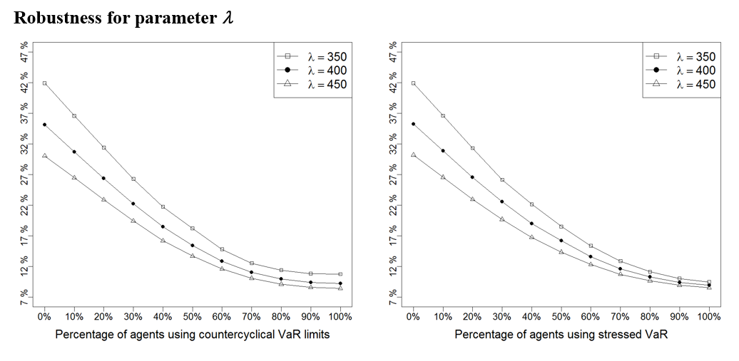
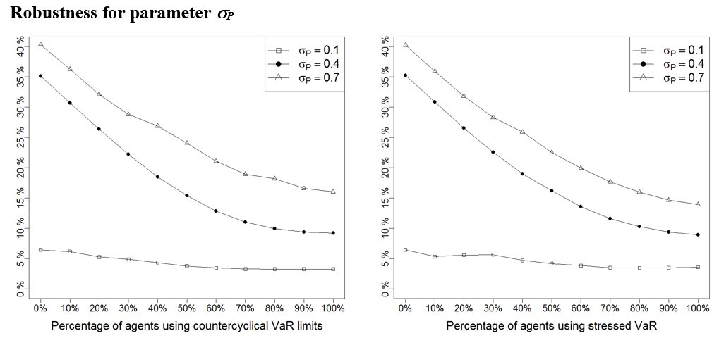
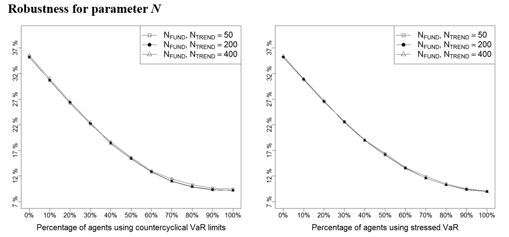
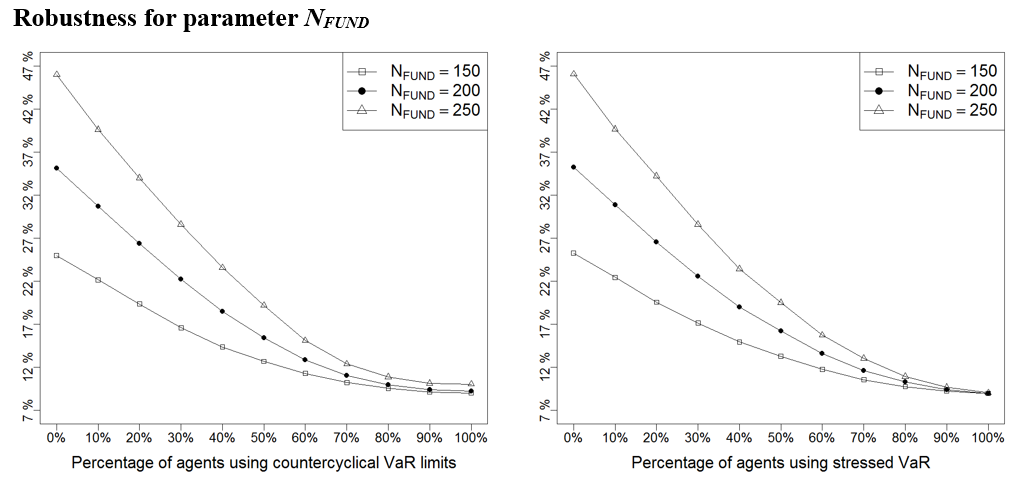
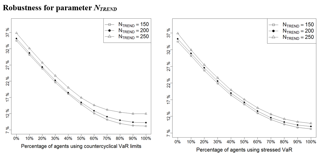
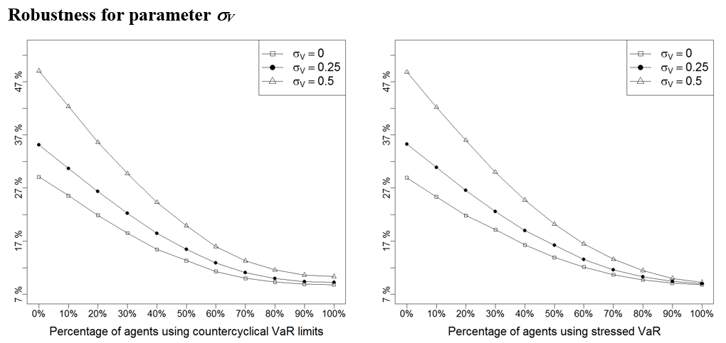
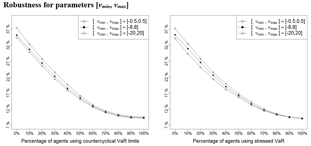
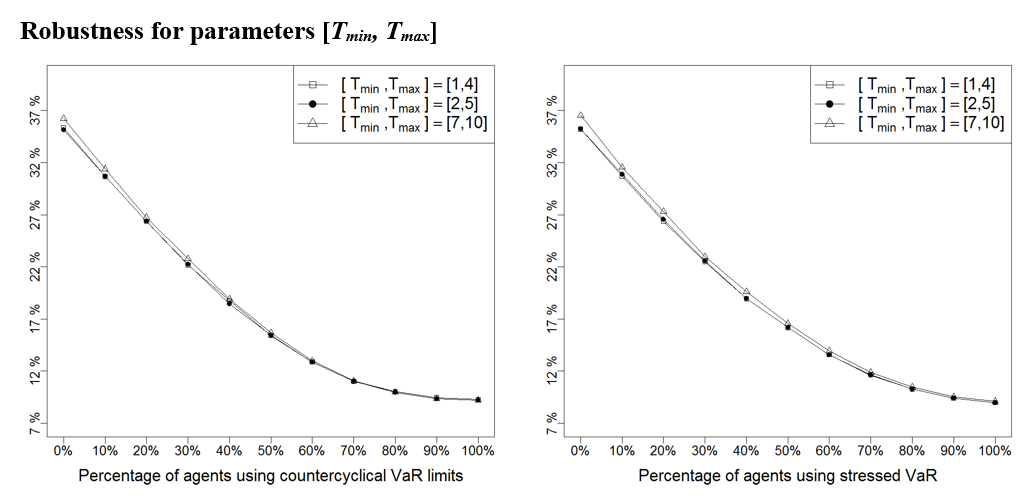
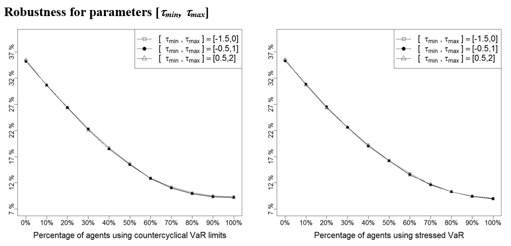
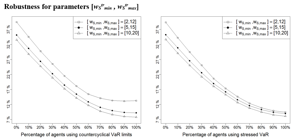
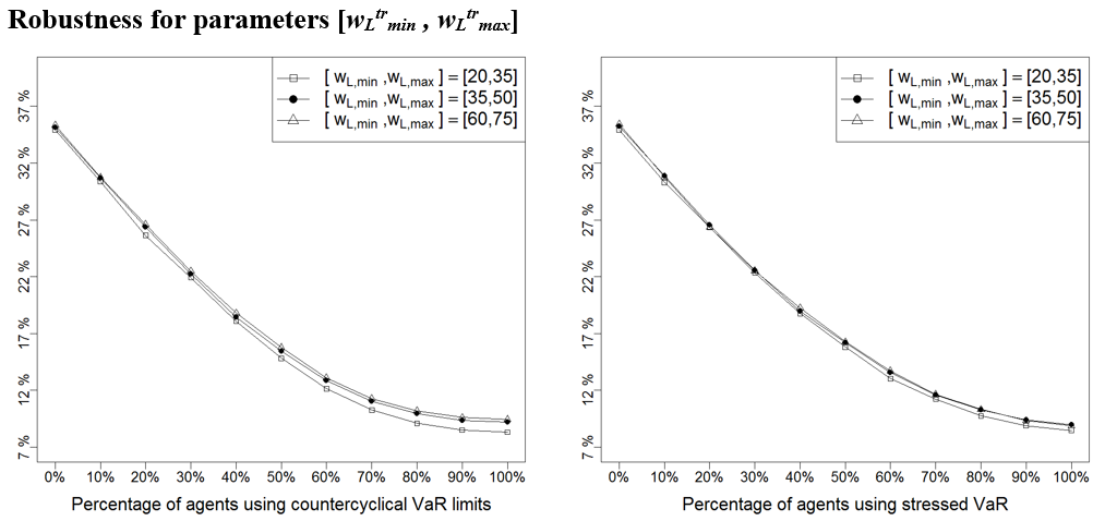
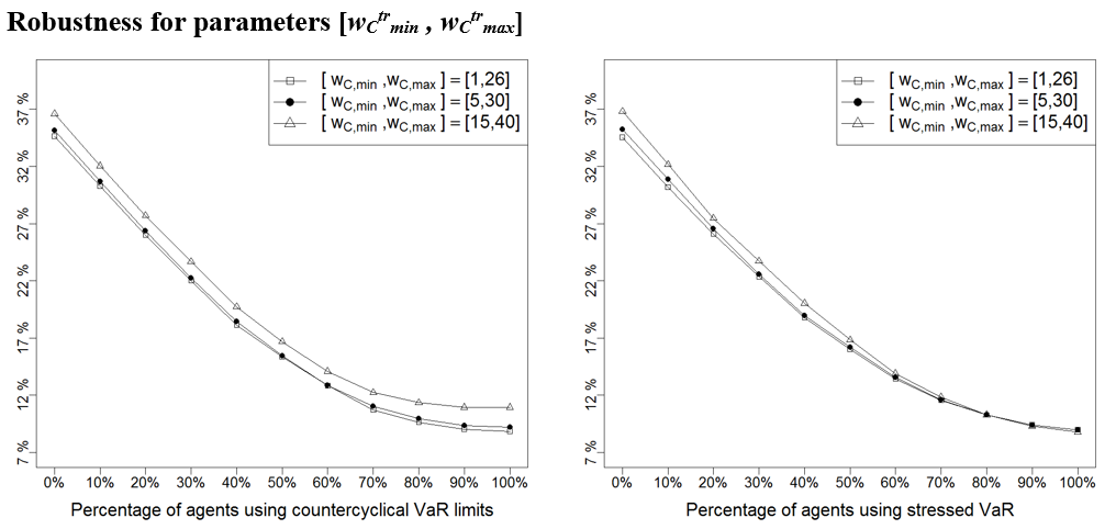
One difficulty associated to agent-based models is the calibration of the usually numerous set of parameters against real data (Thurner 2011). In this section we analyse the robustness of the model results with respect to changes in parameter values. To this aim, we perform a sensitivity analysis using the one-factor-at-a-time methodology (Ten Broeke et al. 2016), varying one parameter at a time to observe its impact on results.
We use an extreme case analysis (Taylor 2009) where we choose an upper and lower bound for each parameter and re-run the experiments to compare the results with the base case shown in section 4. The extreme bounds have been selected as the lowest and highest values of each parameter (1) that make sense (e.g., the long-term window used by technical traders cannot be smaller than the short-term window), and (2) for which the basic model where agents use no VaR still satisfies the stylised facts replicated by our model (for a description of these stylised facts, see (Llacay & Peffer (2018)).
Next, we repeat the experiments done in Sections 4.4-4.21 for the three values of parameters: the base value, the lower bound and the upper bound. In Figure 17 – Figure 28 we provide a summary of the results: to avoid repetitive figures we only show the effect on return volatility as the other instability indicators behave similarly; we have moreover opted for representing only the mean of this indicator (instead of the entire boxplot as in Figure 12 – Figure 14) because this allows to neatly present the results under the three scenarios – base, low, and high value of each parameter – on a single graph and facilitates their comparison. As it can be seen below, it turns out that results are robust to other parameter choices, as Figure 17 – Figure 28 show the same qualitative behaviour than those shown in Section 4.
Table 5 summarises the value of all the parameters used in the robustness analyses shown in Figure 17 – Figure 28.
| Parameter | Base value | Lower bound | Upper bound | Parameter description |
| \(\lambda\) | 400 | 350 | 450 | Liquidity |
| \(\sigma_P\) | 0.4 | 0.1 | 0.7 | Standard deviation for random term in price formation |
| \(N\) | 50 | 200 | 400 | Number of agents, both in the fundamentalist and technical group |
| \(N_{\textit{FUND}}\) | 200 | 150 | 250 | Number of fundamentalist traders |
| \(N_{\textit{TREND}}\) | 200 | 150 | 250 | Number of technical traders |
| \(\sigma_V\) | 0.25 | 0 | 0.5 | Standard deviation for random term in fundamental value formation |
| \([v_{\min}, v_{\max}]\) | [-8, 8] | [-0.5, 0.5] | [-20, 20] | Boundaries of the uniform distribution that sets the difference between the fundamental value and the value perceived by each fundamentalist trader |
| \([T_{\min}, T_{\max}]\) | [2, 5] | [1, 4] | [7, 10] | Boundaries of the uniform distribution that sets the entry thresholds of fundamentalist traders |
| \([\tau_{\min}, \tau_{\max}]\) | [-0.5, 1] | [-1.5, 0] | [0.5, 2] | Boundaries of the uniform distribution that sets the exit thresholds of fundamentalist traders |
| \([w_{S \min}^{tr}, w_{S \max}^{tr}]\) | [5, 15] | [2, 12] | [10, 20] | Boundaries of the uniform distribution that sets the window of short-term moving average used by technical traders |
| \([w_{L \min}^{tr}, w_{L \max}^{tr}]\) | [35, 50] | [20, 35] | [60, 75] | Boundaries of the uniform distribution that sets the window of long-term moving average used by technical traders |
| \([w_{C \min}^{tr}, w_{C \max}^{tr}]\) | [5, 30] | [1, 26] | [15, 40] | Boundaries of the uniform distribution that sets the window of exit channel used by technical traders |
References
ARTHUR, W., Holland, J., LeBaron, B., Palmer, R., & Tayler, P. (1996). Asset pricing under endogenous expectations in an artificial stock market. SFI Working Paper, 96-12-093.
AYMANNS, C., & Farmer, J. (2015). The dynamics of the leverage cycle. Journal of Economic Dynamics and Control, 50, 155-179.
BANK OF ENGLAND. (2004). Financial stability review - December 2004. Bank of England.
BASEL COMMITTEE ON BANKING SUPERVISION. (2009a). Amendment to the capital accord to incorporate market risks. Basel: Bank for International Settlements.
BASEL COMMITTEE ON BANKING SUPERVISION. (2009b). Revisions to the Basel II market risk framework. Basel: Bank for International Settlements.
BASEL COMMITTEE ON BANKING SUPERVISION. (2010). Basel III: A global regulatory framework for more resilient banks and banking systems. Basel: Bank for International Settlements.
BASEL COMMITTEE ON BANKING SUPERVISION. (2017). Implementation. Range of practices in implementing the countercylical capital buffer policy. Basel: Bank for International Settlements.
BECK, T., De Jonghe, O., & Schepens, G. (2011). Bank competition and stability: Cross-country heterogeneity. Retrieved June 14, 2013, from VOX CEPR's Policy Portal: http://www.voxeu.org/article/bank-competition-and-stability-cross-country-heterogeneity. Archived at http://www.webcitation.org/6ils2b4rX.
BONENKAMP, U. (2010). Combining Technical and Fundamental Trading Strategies. Heidelberg: Gabler.
BRUNNERMEIER, M., & Pedersen, L. (2009). Market liquidity and funding liquidity. The Review of Financial Studies, 22(6), 2201–2238.
CHOUDHRY, M. (2013). An Introduction to Value-at-Risk. 5th ed. Chichester: John Wiley & Sons.
CINCOTTI, S., Raberto, M., & Teglio, A. (2011). The EURACE macroeconomic model and simulator. 16th IEA World Congress 2011. Beijing.
CINCOTTI, S., Raberto, M., & Teglio, A. (2012). Macroprudential policies in an agent-based artificial economy. Revue de l'OFCE, 5(124), 205-234.
CLEGG, R. (2006). A practical guide to measuring the Hurst parameter. 21st UK Performance Engineering Workshop, School of Computing Science Technical Report Series, CSTR-916, (pp. 43-55). Newcastle.
CONT, R. (2001). Empirical properties of asset returns: stylized facts and statistical issues. Quantitative Finance, 1, 223-236.
CRISTELLI, M. (2014). Complexity in Financial Markets. Berlin/Heidelberg: Springer.
DA SILVA, M., & Lima, G. (2015). Combining monetary policy and prudential regulation: An agent-based modeling approach. Brasilia: Banco Central do Brasil - Working paper 394.
DANIELSSON, J. & Shin, H. S. (2003). Endogenous risk. In P. Field (Ed.), Modern Risk Management: A History, (pp. 297–316). London: Risk Books.
DANIELSSON, J., Embrechts, P., Goodhart, P., Keating, C., Muennich, F., Renault, O., et al. (2001). An academic response to Basel II. LSE Financial Markets Group.
DE LAROSIÈRE, J., Balcerowicz, L., Issing, O., Masera, R., McCarthy, C., Nyberg, L., et al. (2009). The high-level group on financial supervision in the EU. Brussels.
DUTT, D. (2013). Counter-cyclical financial regulation: Potential for engendering greater stability in the financial system. EY International Congress on Economics I "Europe and Global Economic Rebalancing”. 24-25 October 2013, Ankara.
DYRBERG, A. (2001). Indicators of financial instability. Denmark’s National Bank Monetary Review, April 2001.
EUROPEAN CENTRAL BANK. (2007). Financial stability review - June 2007. Frankfurt: European Central Bank.
EINARSSON, R. (2013). Reproducing the stylized facts of financial returns. Göteborg: Chalmers University of Technology.
EUBANKS, W. (2010). The status of the Basel III Capital Adequacy Accord. CRS Report for Congress.
FAGIOLO, G., & Roventini, A. (2017). Macroeconomic Policy in DSGE and Agent-Based Models Redux: New Developments and Challenges Ahead. Journal of Artificial Societies and Social Simulation, 20.
FARMER, J., & Joshi, S. (2002). The price dynamics of common trading strategies. Journal of Economic Behavior and Organization, 49(2), 149-171.
FINANCIAL SERVICES AUTHORITY. (2009). The Turner review: A regulatory response to the global banking crisis. FSA.
FRANKE, R., & Westerhoff, F. (2012). Structural stochastic volatility in asset pricing dynamics: Estimation and model contest. Journal of Economic Dynamics and Control, 36(8), 1193-1211.
GADANECZ, B., & Jayaram, K. (2008). Measures of financial stability - A review. IFC Bulletin No. 31.
GOODHART, C. (2009). Procyclicality and financial regulation. Estabilidad Financiera, 16, 11-20.
GRIFFITH-JONES, S., & Ocampo, J. (2009). Building on the counter-cyclical consensus: A policy agenda. Brussels: Foundation for European Progressive Studies.
GRIFFITH-JONES, S., & Ocampo, J. (2014). Helping control boom-bust in finance through countercyclical regulation. In G. Cornia, & F. Stewart (Eds.), Towards human development: New approaches to macroeconomics and inequality (pp. 269-289). Oxford: Oxford University Press.
HALDANE, A., & May, R. (2011). Systemic risk in banking ecosystems. Nature, 469(7330), 351.
HERMSEN, O. (2010). Does Basel II destabilize financial markets? An agent-based financial market perspective. The European Physical Journal B, 73(1), 29–40.
HERMSEN, O. (2012a). Does Basel III improve financial market stability? A comparison with the Basel II framework. In The Influence of the Basel II and III Frameworks on Financial Market Stability, pp. 75-114.
HERMSEN, O. (2012b). Effects of the new capital requirements of Basel III on financial market stability. In The Influence of the Basel II and III Frameworks on Financial Market Stability, pp. 115-155.
HOUSE OF LORDS. (2013). Proprietary trading. Parliamentary Commission on Banking Standards.
INTERNATIONAL MONETARY FUND. (2006). Financial soundness indicators – Compilation Guide. Washington D.C.: International Monetary Fund.
INTERNATIONAL MONETARY FUND. (2007). Global financial stability report – October 2007. Washington D.C.: International Monetary Fund.
JOHNSON, N., Jefferies, P. & Ming Hui, P. (2001). Value at Risk: The New Benchmark for Managing Financial Risk. McGraw-Hill: New York, NY.
JOHNSON, N., Jefferies, P., & Ming Hui, P. (2003). Financial Market Complexity. New York: Oxford University Press.
JORION, P. (2001). Value at Risk: The New Benchmark for Managing Financial Risk. New York: McGraw-Hill.
KESTNER, L. (2003). Quantitative Trading Strategies. New York: McGraw-Hill.
KOWALIK, M. (2011). Countercyclical capital regulation: Should bank regulators use rules or discretion? Economic Review, Federal Reserve Bank of Kansas City, Second Quarter 2011.
KRUG, S., Lengnick, M., & Wohltmann, H. (2014). The impact of Basel III on financial (in)stability: An agent-based credit network approach. Kiel: Christian-Albrechts-University - Economic working paper 2014-13.
LLACAY, B. (2015). El impacto de las técnicas VaR en los mercados financieros. Enfoque basado en la simulación multiagente. PhD Thesis, Universitat de Barcelona.
LLACAY, B. & Peffer, G. (2018). Using realistic trading strategies in an agent-based stock market model. Computation and Mathematical Organization Theory, 24(3), 308-350.
LOBANOV, A. (2012). Current trends in prudential regulation of market risk: From Basel I to Basel III. In D. Sornette, S. Ivliev, & H. Woodard (Eds.), Market Risk and Financial modeling (pp. 129-139). Berlin/Heidelber: Springer.
LUX, T., & Marchesi, M. (2000). Volatility clustering in financial markets: A microsimulation of interacting agents. International Journal of Theoretical and Applied Finance, 3(4), 675-702.
MADHAVAN, A. (2000). Market Microstructure: A Survey. Los Angeles: Marshall School of Business.
MALKIEL, B. (1973). A Random Walk Down Wall Street. New York: Norton.
MANAMPERI, N. (2015). A comparative analysis on US financial stress indicators. International Journal of Economics and Financial Issues, 5(2), 613–623.
MCCOY, P. (2015). Countercyclical regulation and its challenges. Boston: Boston College Law School.
MILTON, A. (2016). Day trading with Donchian channels. Retrieved February 20, 2017, from The Balance: https://www.thebalance.com/day-trading-with-donchian-channels-1031186.
MORRIS, S., & Shin, H. (2000). Market risk with interdependent choice. Conference on liquidity risk. Frankfurt.
MURPHY, J. (1999). Technical analysis of the financial markets. Paramus: New York Institute of Finance.
O'NEILL, B. (2011). Fundamentals of the Stock Market. Network, NY: McGraw-Hill.
PERICOLI, M., & Sbracia, M. (2010). Crowded trades among hedge funds. Banca d’Italia Working Paper.
PERSAUD, A. (2000). Sending the herd off the cliff edge: The disturbing interaction between herding and market-sensitive risk management practices. The Journal of Risk Finance, 2(1), 59-65.
PETERS, E. (2014). Stable vs. unstable markets: A tale of two states. First Quadrant.
POPOYAN, L., Napoletano, M., & Roventini, A. (2016). Taming macroeconomic instability: Monetary and macro prudential policy interactions in an agent-based model. Pisa: Scuola Superiore Sant'Anna - LEM working paper 2015/33.
REBONATO, R. (2007). Plight of the Fortune Tellers: Why We Need to Manage Financial Risk Differently. Princeton, NJ: Princeton University Press.
REN, H. (2011). Countercyclical financial regulation. The World Bank - Policy Research Working Paper 5823.
REPULLO, R., & Saurina, J. (2011). The countercyclical capital buffer of Basel III: A critical assessment. Madrid: CEMFI Working Paper No. 1102.
SAITA, F. (2007). Value at risk and bank capital management: Risk adjusted performance, capital management and capital allocation decision making. San Diego: Academic Press.
TAYLOR, M. (2009). What is sensitivity analysis? What is...? Series, 1-8.
TAYLOR, S. (2005). Asset Price Dynamics, Volatility, and Prediction. Princeton, NJ: Princeton University Press.
TEN BROEKE, G., van Voorn, G., & Ligtenberg, A. (2016). Which sensitivity analysis method should I use for my agent-based model? Journal of Artificial Societies and Social Simulation, 19(1), 5.
THE UNIVERSITY OF WARWICK. (2009). The Warwick Commission on International Financial Reform: In Praise of Unlevel Playing Fields. Coventry: The University of Warwick.
THE WORLD BANK. (2013). Global financial development report - Financial stability. Retrieved May 24, 2013, from Key terms explained: http://go.worldbank.org/EXTW5ZJ4C0. Archived at: http://www.webcitation.org/6ilvSzfkV.
THURNER, S. (2011). Systemic financial risk: Agent based models to understand the leverage cycle on national scales and its consequences. IFP/FGS Working Paper, 14.
TSAY, R. (2005). Analysis of Financial Time Series (2nd ed.). Hoboken, NJ: Wiley.
UNITED NATIONS. (2009). Report of the Commission of Experts of the President of the United Nations General Assembly on Reforms of the International Monetary and Financial System. New York: United National.
WHITEHEAD, C. (2013). Destructive coordination. Cornell Law Review, 96, 323-364.