
Introduction
The adverse health effects of pollutants are an important concern for our society. Industry, power plants, vehicles, and domestic appliances emit pollutants that lead to smog, haze, and acidification in the urban atmosphere (Guarnieri & Balmes 2014). The effect of some pollutants is extremely dangerous, because pollutants are generally invisible and can easily penetrate and accumulate in the human body, regardless of the type of substance, either particulates or gases. Their toxicity may eventually lead to various symptoms, such as cardiovascular or pulmonary diseases (Guarnieri & Balmes 2014; Wardekker et al. 2012).
The resulting health issues may vary according to the ambient pollution levels but also by people’s travel patterns. Many public health studies have investigated personal exposure patterns using surveys, mobile gadgets, or backpack sensors, but less attention has been paid to determining how different social groups move in a continuous space or which trajectories through which particular areas cause high exposure.
Another concern is how individual behaviour and socioeconomic status can affect and be affected by pollution exposure. For instance, residents near polluted areas are more likely to be exposed as well as to be socially deprived (David & Don 2012; Kan & Chen 2004; Kan et al. 2008; O’Neill et al. 2003). These problems, therefore, have highlighted the need to discover vulnerabilities to pollution across populations and to develop tools to help prevent future health problems.
Quantifying health response to pollution exposure already involves a high degree of uncertainty (Dias & Tchepel 2018), and studying it at the population level introduces further assumptions in terms of social and individual characteristics and the structural dynamics of urban growth. However, although the impacts on health may be hard to deal with, the patterns of exposure may become clearer when modelled at the individual level, and it seems plausible that higher exposure levels are more likely to lead to disease.
Given that agent-based models (ABMs) are capable of simulating travel patterns with some structure, this study investigates the potential vulnerability to long-term particulate exposure in Seoul, South Korea. The specific research questions are 1) how does the socioeconomic background potentially affect health outcomes and 2) how could these health levels change under different pollution development scenarios? To answer these questions, we developed a proof-of-concept agent-based model (ABM) that measures population vulnerability through various scenarios in two districts of Seoul.
The remainder of this study is structured as follows. In Section 2, we briefly describe the background of individual exposure studies and review ABMs that are closely associated with health. Section 3 provides an introduction to our two study sites, Gangnam and Gwanak, which represent a wealthy and a deprived district in Seoul, respectively, along with a list of our data sets. In Section 4, we describe the model of the two districts and the scenarios for pollution development. Section 5 compares a measure of the potential risk to health by district, sub-district, age, and education between the two districts and presents a map of their spatial distribution. Concluding remarks and suggestions for future work are then discussed in Section 6.
Background: Air Pollution Exposure and Agent-Based Models
The spatial and temporal dynamics of air pollution exposure
Exposure to air pollution takes place when a person inhales harmful pollutants in a location where there are perceptible amounts of toxins in the air. According to Ott, Steinemann, & Wallace (2006), there are two fundamental points to check to model the level of exposure to air pollution effectively: 1) the location of people who are being exposed; and 2) the heterogeneity of pollution concentration in different locations. These questions led to a simple formula, exposure = concentration x time, which in turn was developed into advanced models considering daily behaviour patterns or multiple station data (Dias & Tchepel 2018).
The previous studies in relation to quantifying exposure and health outcomes can be classified into two main streams. Population exposure studies have attempted to associate air pollution with socioeconomic factors, presuming that the social status associated with pollution exposure might have resulted in mortality (or hospital admissions) (Chen, Mengersen, & Tong 2007; Halonen et al. 2016; Wang et al. 2008). These studies used statistical models, including Poisson regression models and generalised linear models, to measure the exposure using patient data or census data. However, using a daily aggregated level of exposure possibly smoothed out the immediate effects of large short-term fluctuations in pollution levels, as well as the characteristic effects of individual in particular locations, which in turn biased the results.
To avoid the ecological fallacy (i.e. assuming individual behaviour can be deduced from data about groups) recent studies have measured personal exposure by exploiting backpack sensors (Langrish et al. 2009; Steinle, Reis, & Sabel 2013), surveys (Beevers et al. 2013; Van Ryswyk et al. 2013), or mobile phones that combine with biomarkers, to demonstrate that where people go is important for their pollution exposure (Dewulf et al. 2016; Dias & Tchepel 2018; Nyhan et al. 2016). Although this approach has widened our spectrum of exposure assessment, many questions remain to be answered. Firstly, without having personal information, it is difficult to know whether people with different personal characteristics (e.g. age, sex, and genetic make-up) or social classes (such as wealth or education level) behave differently, use different modes of transport, or move close to more polluted areas, for example multilane roads and junctions. Additionally, these studies have often been severely time limited. For example, Dewulf et al. (2016) only had two days of mobility data available for research, and Nyhan et al. (2016) measured a week of population-wide PM2.5 exposure. In cases of personal exposure assessment studies in which the causes of symptoms are non-communicable, disease may develop over many years and the exposure levels are subject to high variability of space and time, studies need to be long-term, allowing a history of pollution contact to be developed.
Agent-based models (ABMs) in relation to pollution and health
Agent-based models (ABMs), particularly in pollution studies, have strengths in exploring finely resolved dynamics of long-term individual trajectories in both space and time and the ability to link these directly to the generation of the pollution field, particularly the very significant part of this that relates to transport. This means that we can not only examine passive exposure to pollution when moving to destinations, but also incorporate adaptive behavioural changes and consider possible associated consequences. For example, awareness of exposure to high pollution levels may lead drivers to attempt to alter their commute, thereby changing the places and times of pollution generation and feeding back into further exposure.
Furthermore, we can envisage policy experiments to anticipate the possible effects of road closures, traffic restrictions, or road improvement schemes on the generation of pollution outside protected zones and thereby help to prevent unintended consequences of attempts to control pollution in highly affected areas. The effects of changing transport mode can also be considered; for example, car drivers are typically thought to be more highly exposed to pollution than pedestrians in the same area (Vreeland et al. 2017).
Finally, we can directly address matters of social justice – those who are disadvantaged typically have less power to effect change for themselves than those who are well off and are often also more highly exposed to environmental degradation. With an ABM, we can conduct scenario experiments aimed at improving conditions at the individual level, taking into account age, education level, living and work spaces, and the ability to travel, including the adaptive behaviour of the agents in response to policy changes. In all, the flexibility of ABMs and the ability to estimate uncertainty in scenarios should help to guide our understanding of how pollutant exposure might translate into disease.
Although previous models have thoroughly investigated the detrimental pollution impacts on human health, relatively few have used agent-based modelling (ABM). ABM has perhaps been underused in environmental health disciplines due to either the complexity of dealing with heterogeneous individuals moving through complicated geographies or the lack of sufficiently spatially resolved micro-data.
One simple air pollution exposure ABM was a prototype model called Urban Suite-Pollution (Felsen & Wilensky 2007). The idea was to examine the competition between predators (fixed locations emitting pollution) and prey (people’s reproduction) in an enclosed landscape. This model can lead to a form in which the healthy population is sharply reduced due to the pollution and aging effects. Agents can mitigate the pollution effects by planting trees, which are envisaged as being able to help clean up the pollution diffused from point source power plants. However, after testing the model’s sensitivity, it became clear that fluctuations in the population can be dominated as much by the random walk of the population size, when the birth and death rates are nearly equal, as by the effects of pollution. Moreover, there is no link between the population size or agent locations and the generation of pollution, and the effects of other built infrastructure are lacking (in particular roads). Finally, the pollution spreads purely by diffusion from each point; in practice, the effects of wind, rainout, and urban street canyons are likely to be significant. More realistic geographies are needed to make further progress.
More recently, Newth and Gunasekera (2012) developed an urban pollution model (EPICast-API) that calculates human movement, time usage, dose, and response to estimate the mortality rate, respiratory hospital admissions, and emergency room visits in the greater metropolitan area of Sydney. As far as we are aware, this was the first pragmatic ABM to use an entire urban population to investigate pollution vulnerability. However, exploring the relationship between mortality statistics at a coarse grid scale (1.5 km2) and only for a single year may miss the effects of spatial variability and cumulative exposure. In addition, their study did not decompose the results by social class.
While the complexities of the evolution of the urban air pollution field combined with modelling people with different backgrounds present a strong challenge for studies of this type, the small number of existing pollution simulations with ABM suggest that there is hope that more detailed simulations will help us to make progress. Here we attempt to improve on the randomness of agents’ behaviour from the Urban Suite-Pollution model by using origin-destination data from travel surveys, use measured data to estimate the pollution field and increase the spatial resolution of the pollution grid and the temporal resolution relative to the EPICast-API model, whilst also breaking down the population by personal and social characteristics.
Study Area and Data Collection
Study area
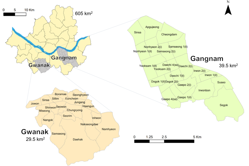
The city of Seoul was selected as a city with a marked pollution problem for which we have appropriate data available. We selected Gangnam and Gwanak districts for a comparative study, largely on the basis of the contrasting character of these two districts (see Figure 1). A district within Seoul is an administrative boundary, of which the functions are equivalent to a county or possibly to a borough in London.
Gangnam is situated in the south-eastern part of Seoul. The area accounts for 39.51km2, constituting 6.5% of Seoul, and about 577,400 inhabitants (Gangnam-Office 2016). There are 22 sub-districts in Gangnam. Once known as a region with farms and livestock, Gangnam has now become the most active business district in Seoul. Several headquarters of the country’s trade, finance, and high-tech industries are concentrated in the core area. Medical services, broadcast and entertainment firms, and state-of-the-art fashions are established here, attracting both domestic and overseas visitors throughout the year. Gangnam also has the highest number of apartments in Seoul, and, due to the shortage of space for both residential and business uses, it suffers from traffic congestion as well as extra pollution during rush hours and at weekends.
Gwanak is located in the south-western part of Seoul (Gwanak-Office 2016). The total area accounts for 29.57 km2 (4.9% of Seoul’s territory and 525,607 inhabitants), but more than half consists of the mountainous area that surrounds Gwanak Mountain (632m), mostly formed across Daehak, Samseong, and Namhyeon. There are 21 sub-districts, including Silim and Jungang, which are near the subway station and are commercial centres. Due to the topographical structure, most people live in the northern part of the district, where there is a large number of single-family and multi-family housing for commuters and university students.
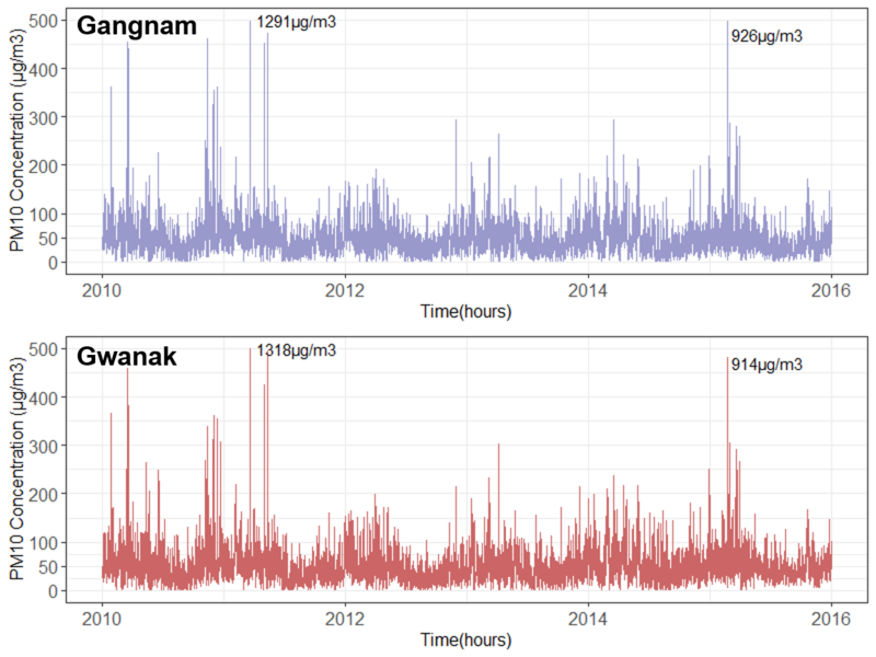
The pollution levels in Gangnam and Gwanak fluctuate by season and day-to-day. Over an annual cycle, the daily averages of PM10 (particulate matter 10 micrometres or less in diameter) tend to peak at 100μg/m3 during the driest period between December and March, while the lowest reach 30μg/m3 during the monsoon period in July and August, when more than 50% of the rainfall (approx. 650 mm per annum) occurs. On the other hand, a daily cycle with hourly time resolution shows more extreme peaks of up to 800μg/m3. This might depend on the traffic volume during rush hours or on the city’s landscape, which may trap polluted air.
Data collection
Table 1 provides an overview of the variables used in this initial model. We collected station data, individual personal attributes, road layouts, land prices, and an origin–destination matrix for daily travel. The data are all stored on our CoMSES website (https://www.comses.net /codebases/cb6c2243-fb44-4543-a372-6fee5f034c40/releases/1.1.0/).
| Components | Variable | Value | References |
| Pollution | PM10 | Numeric | National Institute of Environmental Research |
| Sensitivity | Age | Numeric | Korean Statistical Integrated System (KOSIS) |
| Education | Dichotomous | ||
| Road proximity | Dichotomous | Intelligent Transportation Systems (ITS) | |
| Official land price | Grade | National Spatial Data Integration (NSDI) | |
| Movement | Origin-Destination matrix | Numeric | Korea Transport Database (KTDB) |
At this stage of the model development, we did not track agents’ movement along the road system. However, we included a measure of road proximity as a means of demonstrating the negative impact of enhanced emissions near roadsides, irrespective of social categories. The data were retrieved from the Intelligent Transport Systems (ITS, http://its.go.kr/) institution run by the Korean Ministry of Land and Transport.
For this preliminary research, age and education were the characteristics that featured in pollution sensitivity. Age was included because different age groups presumably have distinctive differences in their physical health status and sensitivity to pollution. The raw data were retrieved from the 2010 Census of the Korean Statistical Office (http://kosis.kr/), which were grouped into five-year intervals (e.g. 0–4, 5–9, 10–14 …). We aggregated the groups into three: 0–15, 15–64, and 65+. The education level was included to represent the awareness of potential harm from pollution. The 2010 census surveyed education status above 10 years of age and provided data in eight categories (primary-school dropout, primary-school graduate, middle-school dropout, middle-school graduate, high-school dropout, high-school graduate, college or university student, over a bachelor’s degree). For simplicity, we aggregated into two groups of above and below middle-school graduation, but we gave randomness to approximate the census.
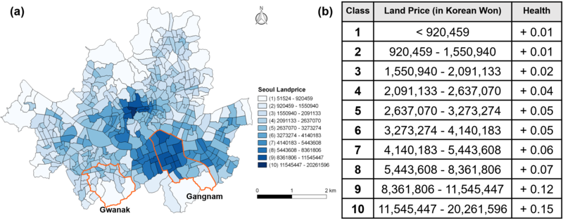
The official land price was selected as an indicator of the ability to recover from pollution impacts. Coffee et al. (2013) attempted to show a relationship between residential properties with high socioeconomic status and health as part of a study of housing properties and social well-being. The reason for using residential property was not only because it represents immovable and location-specific capital but also because of its expression of price in the economy: those who are more able to afford higher-priced housing are also perhaps better able to access health care or to adapt their lifestyle to compensate for high pollution levels. Here, we used official land prices as a proxy for regional socioeconomic status. The 2015 land prices were retrieved from the National Spatial Data Integration website (NSDI, http://www.nsdi.go.kr/). The raw data were given in tables of prices by census block units. Using the natural break method, we aggregated the block units into the sub-district level, then we categorised the price distribution into 10 sub-divisions (see Figure 3 (a)). Figure 3 (b) indicates the hypothetical health changes determined by the land prices. It is assumed that agents’ nominal health level can recover up to a maximum adaptive capacity level at a rate that is higher for those living in areas with higher property values.
Origin–destination matrices for Gangnam and Gwanak were downloaded from the Korean Transportation Database (https://www.ktdb.go.kr) and converted into fractions so that we could allocate home locations and associated work locations to a sub-sample of the total population.
Model Description
In this section, we describe our pollution exposure model based on the ODD protocol (Grimm et al. 2006, 2010). The source codes, along with the extended ODD protocol, are available from CoMSES (https://www.comses.net/codebases/cb6c2243-fb44-4543-a372-6fee5f034c40 /releases/1.1.0/). The model was implemented in NetLogo 6.0.4, each district being run as a separate self-contained model: this means that some agents with home locations within a district but work destinations in another district had to be excluded from consideration. We implemented 9 scenarios for 100 iterations each in ‘Behaviorspace’ embedded in NetLogo, then we analysed the outcomes with ‘tidyverse’ in R 3.4.4 (Wickham 2017).
Model purpose
The model’s objective is to understand the cumulative effects on population vulnerability from exposure to PM10 by different age and educational groups in both Gangnam (wealthy) and Gwanak (deprived) districts.
Entities, state variables, and scales
For the sake of speed we used a 1% population sample of agents (individuals) in each district to generate a simple synthetic population in Gwanak district and Gangnam district. For example, the total population of Boramae (one of the sub-districts of Gwanak) consisted of 24,351 persons, of whom 2,219 (9%) were aged under 15 (excluding infants under 5), 19,520 (80%) were aged between 15 and 64, and 2,612 (11%) were aged 65 or above. In the model, each group was converted into 22, 195, and 26 people, respectively. Hence, the total population of Gangnam was converted into 5050 agents and that of Gwanak into 4915 agents. Each agent has a list of attributes that includes the name of the home location, coordinates of the home location, name of the destination, coordinates of the destination, age group (i.e. young, active, or old), education level, and health. Every agent will move to his or her given destination location during working hours and return home again on alternate model ticks (see more details in Section 4.3).
We assumed that the agents have not experienced any previous exposure, as we lack either health records or exposure histories for the population. Our simulation is thus only able to track the likely rate at which exposure effects accumulate over time in a given district relative to others. Depending on the way in which this simulated history works, we hope to be able to estimate the accumulated risk that an unexposed population would have developed over the period of the simulation. Each agent is assigned a nominal ‘health’ level, which is an integer with an initial value of 300. Depending on their socioeconomic status, they will lose health when exposed to a PM10 over a threshold near 100μg/m3. We chose this as it is a Korean hourly ambient air quality standard (https://www.airkorea.or.kr/eng/information/airQuality Standards), although the lack of data on how this relates to disease means that the relation to the actual health impact is not entirely clear. We assumed, consistent with the idea of an air quality standard, that the adverse effects on health only begin to operate when pollution is above this threshold. More details on this matter are given below.
In addition to PM10 exposure, we included sensitivity as a modifier of the adverse factors degrading the agents’ health and used the land price as a recovery factor. Sensitivity is composed of two socioeconomic attributes of an agent that control the degree of health loss. One determinant is age, which works as a proxy for physical health variance, assuming that very young or very old population members are more likely to suffer when exposed to pollutants. The other is educational level, designed to take into account a possible lack of pollution awareness amongst those with lower educational depth. By contrast, the land price is a proxy for health recovery based on the idea that medical facilities (e.g. hospitals, clinics, and pharmacies) have greater chances of being located in areas with higher property values or that higher values may mean a greater ability to avoid polluted air, as mentioned above. The model does not consider any transmission effects between individuals or environments, because the diseases resulting from pollution exposure are non-communicable, although, in practice, compromised pulmonary systems may make agents with high exposure more likely to suffer ill effects from viral or bacterial diseases.
Process overview and scheduling
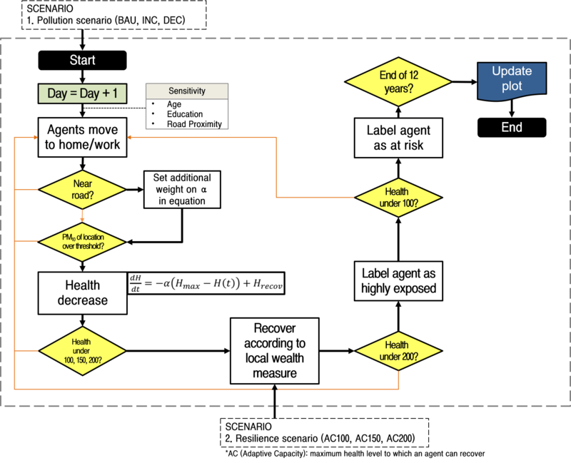
Figure 4 shows the conceptual outline of the model. During the set-up process, every agent is assigned a fixed home name (sub-district) and home patch as well as a destination name and patch. The destination names and patches differ by age group. Agents aged between 15 and 65, also known as the economically active population, will move to their destination patches according to the fraction moving to a given destination in the origin–destination (OD) matrix. Those who commute to other districts are allocated to dummy patches outside the district during working hours – these agents are not included in the overall statistics, as we do not have data for them during the day.
Agents aged under 15 will move to a random patch within radius 3, while those aged over 65 will move to a random patch within radius 1: this is intended to represent a more restricted range of movement for this fraction of the population. As we were not modelling the traffic flow, we simplified movement by translating the agents to their destination patch during the day (one tick) and back to the home patch at night (the next tick). Every agent will start without any medical history and with full health; all are susceptible to local levels of PM10 within their current patch. An additional weight for PM10 is added if the agents are near a road, assuming that the particles from tailpipe exhausts or tyre dust are generated near roads (see the details in Section 4.12). An agent will lose health when exposed to a patch exceeding 100μg/m3 of PM10. Agents in the youngest or oldest age groups, and those with lower educational levels, receive an additional penalty. Recovery can occur according to local property values up to a maximum adaptive capacity (see the details in Section 4.20).
As the agents continue to lose health from a high PM10, we assumed that their health status can change suddenly when they cross a given threshold. Those with health less than two-thirds of the starting value change status to ‘highly exposed’, and those with health less than one-third of the initial value are labelled ‘at risk’. The model terminates either if all the agents turn to the ‘at risk’ status or the end of year 12 is reached, that is, tick 8764.
Pedestrians’ decision-making process
The agents in the model have little by way of reasoning ability. Their behaviour is entirely driven by a simple schedule. Agents, in common, follow the hypotheses mentioned below:
- An agent’s birth, death, and ageing are not considered
- Agents have minimal cognitive representation but understand their area boundaries
- 1 tick is equivalent to half a day, that is, working and home hours
- Every agent starts with a health status of 300, but this drops when the agent is exposed to pollution
- Agents commute to the same location until the simulation ends
- For visualisation purposes, if the health status of an agent drops below 200, the agent’s colour turns purple; when it drops below 100, the colour turns red
- If an agent’s health reaches 0, he or she will be sent to hospital for treatment
- All agents stop if the system reaches 8764 ticks (equivalent to 12 years) or if the ‘at risk’ population reaches 100% of the total population
Given the lack of address information, every agent was randomly distributed in their home location based on the census. Agents aged 15–64 commute within a sub-district but can also move to different sub-districts derived from the origin–destination matrix. Movement is random within these constraints but with an additional tendency to select patches with roads within permitted sub-districts randomly as a way of approximating transportation in the absence of a full traffic model. By contrast, the movement range of the young and the elderly is restricted close to their origin. This is based on the idea that most children go to schools and participate in after-school activities near home and that the elderly are assumed to travel to distant places less frequently. We did not consider agents who commute to different districts outside the study area or the mode of transport for trips (so there is no accounting for differences between pedestrians, car travel, or buses or for the fact that the pollution levels may be lower within buildings). The effect of roads proves to be significant in determining the relative outcomes between groups.
Atmospheric settings
Most pollutants vary quite strongly across location and time. Given that each district has only one background station, estimations of personal exposure based on uniform air quality might overlook a significant amount of variance of pollution across space and time and can under- or overestimate personal exposure levels, particularly when the study region is larger than a census block level (Dias & Tchepel 2018). Hence, rather than allocating a uniform value homogeneously to a region, we allowed each patch to select one value randomly from the daily pollution field measured at the local background station (Figure 5). For example, on the first day of January 2010, each patch would randomly select one of the PM10 values between 09:00 and 19:00. This allows for the likely spatial variability between patches to be preserved rather than all the patches varying in exactly the same way as the local station.
We also applied an additional weight factor of pollution to road exposure, following the evidence that adverse effects on health are more likely to occur in proximity to roads. One of the pieces of evidence from Harrison, Jones, and Lawrence (2004) involves an average mass increment of 11.5μg/m3 of PM10 and an 8.0 μg/m3 increment of PM2.5 between roadside (daily mean 34.7 μg/m3 PM10) and urban background areas (daily mean 23.2 μg/m3) measured at three sample sites in London and one in Leeds. Higher chances of acute illness can happen because of the direct inhalation of toxic fumes inside a vehicle or walking close to vehicle exhausts. In fact, we discovered that the urban roadside stations in Gangnam and Gwanak between 2010 and 2015 showed a 40% and 38% higher concentration of PM10 than the background stations. Thus, we applied these levels to the road patches in each district.

Measurement of exposure
In accordance with the PM10 concentration criteria provided by the Korean hourly ambient air quality standard, the air quality is considered to be harmful when it exceeds 100μg/m3, although the lack of data on how this is linked to disease means that the relation to the actual health impact is not entirely clear.
As mentioned above, since the diseases resulting from pollution exposure are generally non-communicable, at least to first order, the model does not consider any transmission effects between individuals but considers the effects resulting from continuous interactions between individual spatial trajectories constrained by daily activity patterns, with simulated spatial micro-scale atmospheric pollution distributions.
It was assumed that, compared with a healthy person, a person suffering from disease symptoms will lose a steadily greater amount of health the more that he or she is exposed to pollution. For example, an agent with health of 50 will lose health more rapidly than an agent with health of 150 when they are equally exposed to over 100μg/m3of PM10. Accordingly, we set the rate of change of an individual’s health status caused by PM10 exposure to vary linearly with health:
| $$If PM_{10} \geq 100, \, dH/dT = -\alpha(H_{max} – H(t)) + H_{recov}$$ | (1) |
where \(H_{max}\) denotes an agent’s health status at the beginning and \(H(t)\) is strictly less than \(H_{max}\). Thus, in the absence of any recovery and with constant α and PM10 always above the threshold, agents’ health values would decrease exponentially away from their initial value H(0). H(t) is the current health value. The factor α sets the rate of change per unit of time when the health impact applies. This factor is chosen from a random uniform distribution between zero and a maximum on each tick to allow for the fact that, even within a patch, since these are 30m across, the individual exposure levels will be very different. To some extent, this mimics the fact that people may move in and out of buildings, for example. For vulnerable populations, we apply the first term in Equation 1 again (so, for example, an agent in the youngest age group has double the probability of experiencing an effect). \(H_{recov}\) is a health recovery rate that varies by the real estate price of the agent’s home location, as in Figure 3, up to a maximum adaptive capacity (AC, i.e. recovery can only increase health up to some scenario-dependent value). For road patches, we add to alpha an extra value slightly larger than that of non-road patches, i.e. roads have slightly more than double the impact of non-road areas. Additionally, the pollution levels are inflated as mentioned in Section 4.12.
Overall, this gives us a threshold model in which impacts begin to accumulate whenever the air quality is marked as unhealthy. However, random variations are applied both to the above agent selection and to the health impact to allow for the fact that the exposure will not be uniform across agents, even when they are more or less spatially co-located (e.g. they may be inside or outside a building or inside a vehicle rather than walking at the roadside).
Scenario description
This study set three scenarios for pollution trends and three scenarios for adaptive capacity control (see Table 2). These were mainly designed as ‘what if’ scenarios to explore possible consequences in the future. We tested pollution scenarios as a means of showing how the constant upper or lower trend of PM10 can trigger the population’s acute illness. Resilience scenarios can be used as an indicator to reflect individuals’ health characteristics and the timing of the community response. However, a full sensitivity analysis is beyond the scope of this paper; in this first glance, we simply wished to explore the kinds of effects that the above model set-up produces.
| Type | Description | Count | ||
| PM Control | BAU | INC | NOC | 3 |
| Resilience (AC) | 100 | 150 | 200 | 3 |
Pollution scenarios
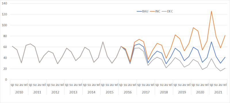
The pollution scenarios consist of business as usual (BAU), increase (INC), and decrease (DEC). BAU refers to ‘What if the seasonal pollution levels continue for another period?’, which assumes that the 6-year time series of hourly PM10 in 2010–2015 will replicate itself for another 6 years. INC projects an upward trend of the seasonal PM10 averages by 3% every season, whereas DEC anticipates an equivalent decrease (see Figure 6).
Resilience scenarios
These scenarios change the ‘adaptive capacity’ (i.e. the maximum health to which recovery is possible for an agent, hereinafter AC) of 100, 150, and 200. This simulates mitigating measures, such as improved treatment for the effects of exposure. As a brief illustration, if the resilience is set for AC100, an agent whose health drops below 100 will try to recover up to a maximum of 100.
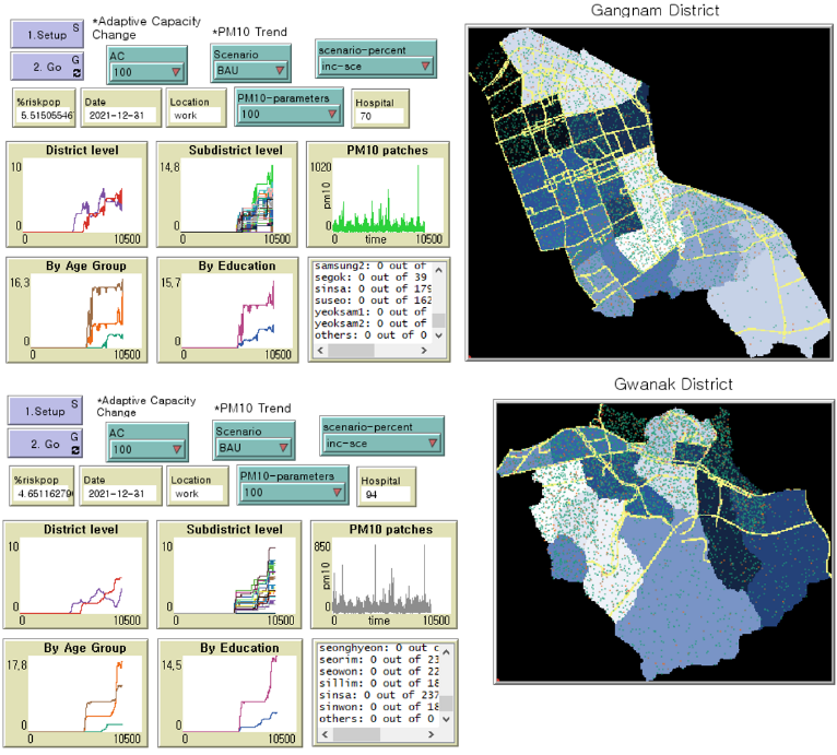
Model interface
The model environment was derived from a GIS data set of each district (see Figure 7). For simplicity, we excluded building and traffic information for the present. The spatial extent of Gangnam and Gwanak are around 40 km2 and 30 km2, respectively, with a 30 m by 30 m spatial resolution. We used two time-steps per day (i.e. home hours, working hours), and simulated 12 years, of which the earlier 6 years of PM10 were from the observational data set. For the second 6 years, we reused the first 6 years but modified them to create scenarios for future projection.
Simulation Results
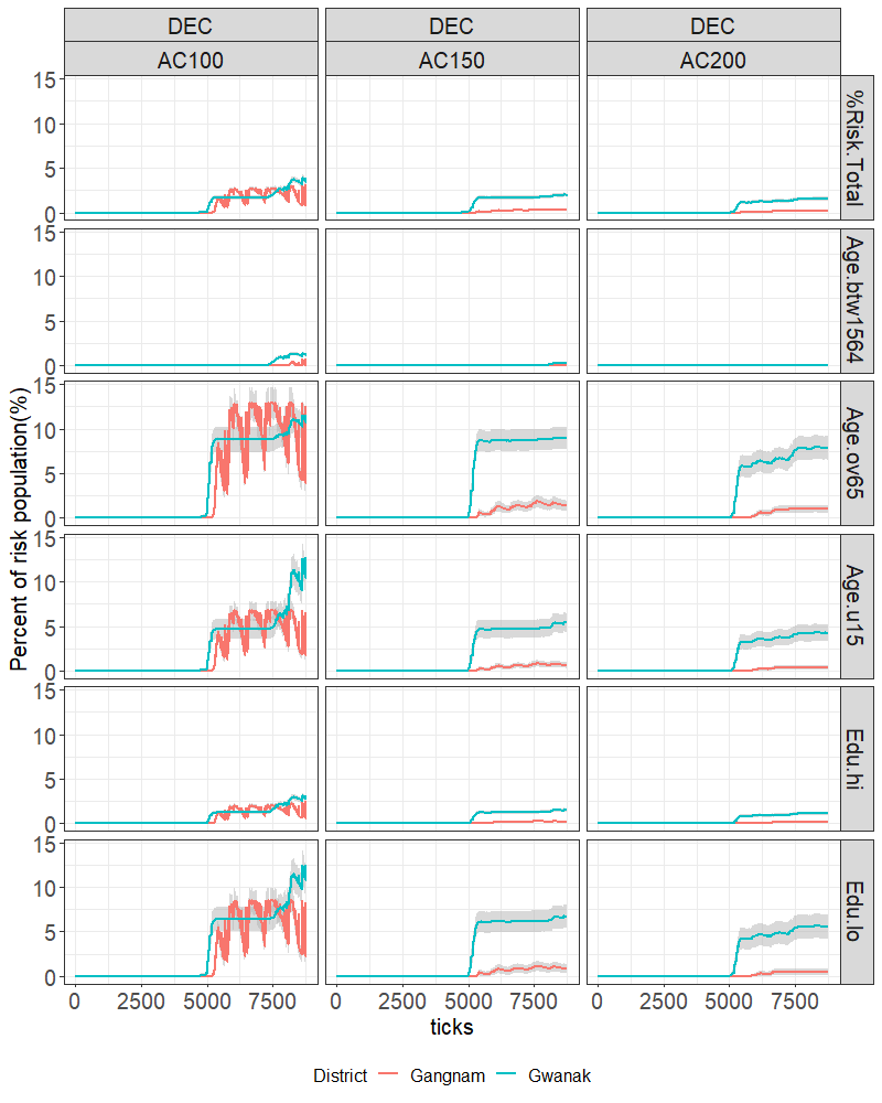
Each district has a combination of 3 categories of pollution scenarios (BAU, INC, and DEC) and 3 resilience scenarios (AC100, AC150, and AC200). For each scenario has we plot time on the x-axis and the proportion of population at risk on the y-axis, where “at-risk” refers to agents whose health status is below 100. We ran all the parameter combinations (e.g. ‘BAU \(\times\) AC100’) 100 times and show the mean value for each.
A comparison of health vulnerability in two districts
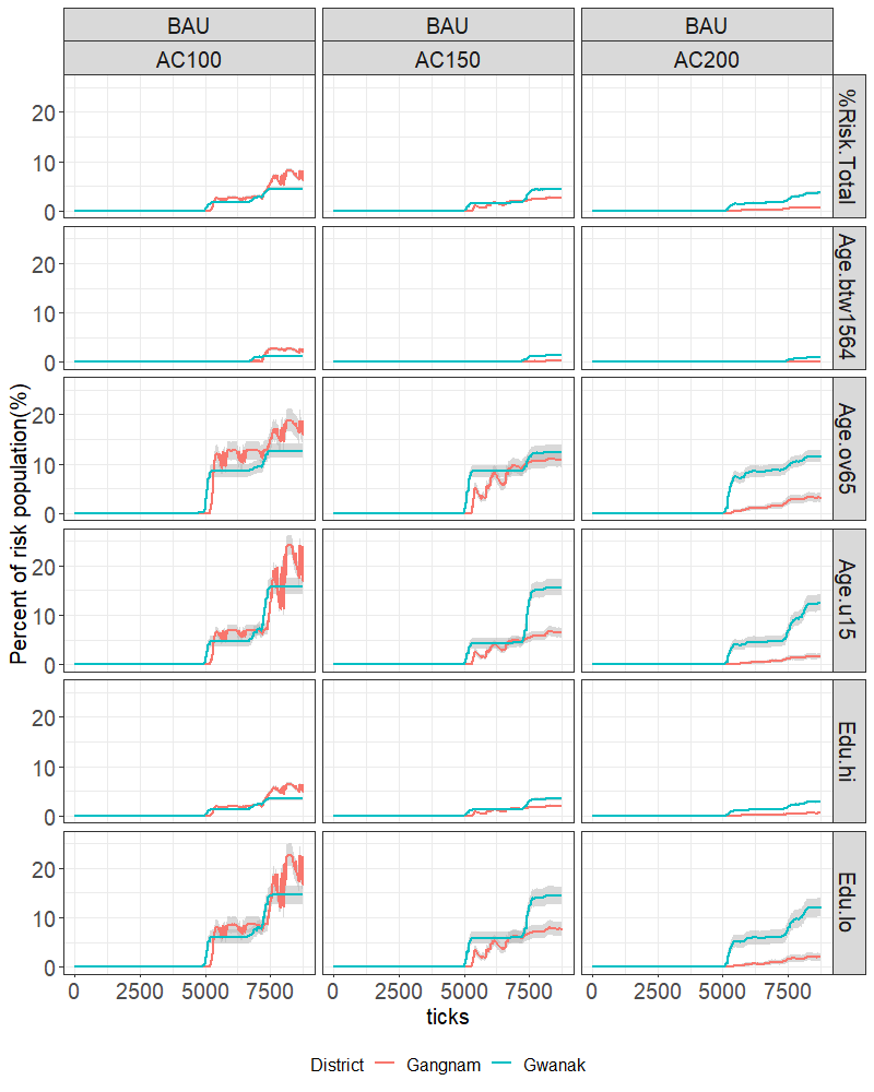
We compared the overall trend of health vulnerability in the two districts by age groups and educational levels (Figure 8). We show the average percentages at risk for the total population, and then percentages within each sub-group relative to the size of the sub-group population. The grey bands show the spread (one standard deviation) of results over the 100 runs (sufficient to be sure that stochastic fluctuations in the means were not significant). Results are plotted with a different colour for each district.
BAU scenario
In the BAU scenario, in which 6 years of PM10 records were assumed to be replicated for another 6 years, the risk population in both districts simultaneously started to increase after 5000 ticks (see Figure 8). This might be expected as the health conditions were given to the agents equally at the beginning of the simulation and had a similar health reduction range when exposed to the PM10 threshold.
However, the temporal patterns varied by districts. In Figure 8 (a), the total population at risk in Gwanak showed a gradual increase over the duration of the simulation and resulted in an average of 4.9% for AC100 (top left panel, blue line), whereas in Gangnam the increase started slightly later than Gwanak but overtook Gwanak after 7500 ticks and fluctuated until the end of the simulation, resulting in 7.7% for AC100. However, while the total population at risk of Gangnam dropped considerably to 2.19% in AC150 and to 0.7% in AC200, the Gwanak risk population dropped only marginally to 3.84% and 2.4% in each AC150 and AC200 scenario. It seems Gangnam was more sensitive to the adaptive cap: this likely reflects the generally better off nature of the population, so that recovery is more effective if health is allowed to increase to a higher level.
With regard to the age and education results, both Gangnam and Gwanak agents aged 15–64 (“economically active”) as well as highly educated agents faced the lowest risk of the population, as might be expected from the model setup: one could imagine a case in which the active population were more exposed as a result of travel on very polluted highways, or being outdoors in polluted air more, but at least for this simulation this appears not to be the case. Barely anyone in these groups showed illness until 7000 ticks, and less than a percentage difference was measured in the whole run in all the scenarios. By contrast, the risk population aged under 15, aged over 65, or with a low education status rose dramatically after 5000 ticks in both districts, although for Gangnam residents, both groups experienced a repetitive trend of sickness and recovery. The older residents experienced lower levels of fluctuation, but generally reached higher percentage risk levels earlier than the young or less educated.
The fluctuations in Gangnam’s results, mostly in the AC100 scenario and in under 15, aged over 65, and low education, groups seem to be associated with the balance between recovery rate and degrading of health with exposure: in Gwanak recovery is less effective since the population is generally less well off. If the recovery rate is lowered relative to exposure effects, then these oscillations tend not to be observed.
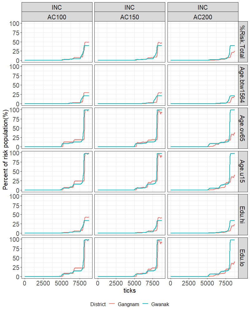
INC scenario
In Figure 9, the risk population in the INC scenario, which assumes a 3% increase in PM10 per season starting from 4383 ticks (i.e. the seventh year), showed a rapid rise just after the onset as well as at the end of the simulation, particularly in the vulnerable groups: those aged under 15, aged over 65, and with a low education level. Note also that the oscillatory behaviour seen in BAU AC100 is now absent. Most of the resilience scenarios did not prevent a severe rise, except the AC200 in Gangnam, where more than half of the population in vulnerable groups managed to recover their health to some extent.
The ‘stepped’-type increase, a reoccurrence of the “increase-stable-increase-stable” pattern visible in Gwanak-BAU-AC150-u15, for example, was also observed in the INC scenario but this time for all scenario combinations. By tracking a sample number of agents, we identified that the initial rise in the risk population was attributable to agents whose home and work areas were close to roads; the following rises were experienced by residents whose either home or work area (but not both) was close to roads.
DEC scenario
In the DEC scenario (see Figure 10), which assumes a 3% decrease in the PM10 per season starting from the seventh year, the risk population in Gangnam fluctuated in the AC100 scenario. Gwanak, on the other hand, presented a stable pattern in the AC100 scenario with only a few fluctuations. However, in the other resilience scenarios, we did not see an extreme rise in the number of ill people, although nearly 10 percent of the elderly population remained at risk. We did not notice an extreme rise in the number of ill people in Gangnam, except for 3 per cent of the elderly and low-educated population, whose health status was constantly at risk.
Health vulnerability within districts
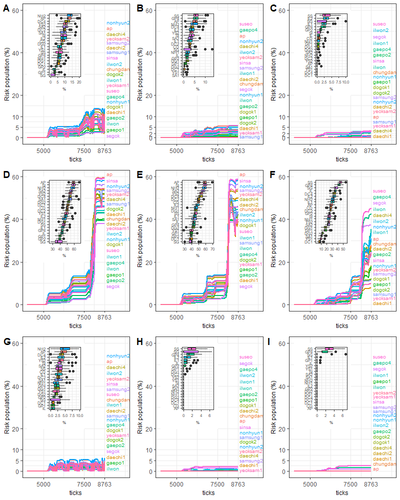
A sub-district-level analysis was conducted to compare vulnerable areas within a district. Sub-district boundaries appear in Figure 7 marked on yellow on the two maps to the right. As with the regional analysis, an average value from 100 iterations was calculated and illustrated (see Figure 11 and Figure 12). Since Gangnam and Gwanak are composed of 22 and 21 sub-districts, respectively, we added inset boxplots of risk population outcomes to summarise the results.
Gangnam
Figure 11 shows that there is considerable geographical variation within districts, but those areas highly ranked by risk also varied distinctively by pollution scenario. The most frequently referred-to areas were Nonhyun2, Apgujeong, Daechi4, and Yeoksam2, where there were complex road networks (see Figure 11 and the ODD document). It was also remarkable that the highest-ranked areas indicated in the AC100 scenarios (i.e. Figure 11 A, D, and G) suddenly dropped to the lower quantile in AC200 (i.e. Figure 11 C, F, and I). On the other hand, some low ranked (but low population) sub-districts (e.g. Segok) moved up significantly in risk ranking.
The BAU scenarios showed fluctuations throughout the simulation, but the fluctuation range was as usual the largest at AC100. As mentioned in Section 5.1, the fluctuation range was due to the constant repetition of health degradation and recovery of agents whose home or work location is close to a high density of road networks. In five sub-districts the population at risk exceeded 10%, including Nonhyun2 (13.4%), Apgujeong (12.8%), Daechi4 (11.6%), Yeoksam2, and Samsung2 in the AC100 scenario. However, the people at risk in these areas dropped significantly below 5% in AC150 and finally fell close to 0% in the AC200 scenario to become one of the areas without a population that exceeds our risk threshold.
In the INC scenarios, in which the most vulnerable areas surged to 40% after 8000 ticks (see more details in Figure 11 D, E, and F), the most/least vulnerable districts again changed significantly with AC, and with a similar pattern. In all the districts, it was clear that the vulnerable groups aged under 15, aged over 65, with a lower education level, and dwelling or commuting close to roads have a tendency to become unwell in the first instance, then the people who either are classified as one of the groups or move to nearby roads tend to be the next people to be affected detrimentally by PM10, and finally a major population with potentially unwell people degrades suddenly, experiencing a remarkable increase in the risk population. At the final tick (day), 20 sub-districts in AC100, 18 districts in AC150, and 2 districts in AC200 had more than 40% of the population at risk. Hence, even though residents of Gangnam had a greater chance of recovery in Seoul, the district still would not avoid the possibility of having a very considerable number of population members at risk as a result of pollution exposure. In the DEC scenario, all districts have relatively low risk, although again for AC100 Nonhyun1 is the most affected areas, but for AC150 and 200 Suseo, Segok, and Gaepo4 stand out.
Gwanak
In all scenario results, Jungang, Sillim, Euncheon, Jowon, and Sunghyun were the most highly ranked sub-districts to have a risk population across all the scenarios. One of the geographical features of these areas is the blending of residential and commercial development zones, implying that the likelihood of high exposure can occur as a result of high traffic during busy hours. The lowest risk group consistently included areas such as Daehak, Nanhyang, Nangok and Namhyeon. This stability with scenario contrasts markedly with Gangnam, most likely as a result of the much weaker ability of residents in Gwanak to recover from exposure generally.

Conclusion and Future Work
This study was the first attempt to evaluate the health vulnerability of urban residents in Seoul during long-term exposure to particulates following an agent-based approach. We used three exposure scenarios (i.e. BAU, INC, and DEC) and three resilience scenarios (i.e. AC100, AC150, and AC200) to explore possible future health outcomes in regard to seasonal pollution change and regional resilience. Simulations were conducted in two districts in Seoul, Gangnam and Gwanak.
We initially compared the two districts to investigate how the exposure level and socioeconomic resilience affect the population’s health. Assuming that all agents were initially healthy, and that a tick was equivalent to half a day, it was found that the vulnerability in both districts increased sharply after 5000 ticks in the INC scenarios and the combination of BAU and AC100. These findings extend those of Jerrett et al. (2001), Moreno-Jiménez et al. (2016), and O’Neill et al. (2003), showing that when disparities in health outcomes are likely to depend on socioeconomic status (SES), especially when the group is exposed over a long period geographical factors become important (Brook et al. 2004; Jerrett et al. 2001).
The striking difference between districts was that the vulnerability rate of the group aged under 15, the group aged over 65, and the low-educated group in Gwanak increased by over 10% in the BAU scenarios, over 25% in the INC scenarios, and over 5% in the DEC scenarios regardless of resilience scenarios. By contrast, the rate in Gangnam reduced considerably in the AC200 scenarios. These differences were driven by a range of factors, including the differences in the road layout, population composition, pollution loading, recovery rate and range of activity, although the importance of the various factors remains to be investigated. At least in this model good access to measures that enable recovery from the impacts of air pollution, especially where this can lead to a recovery nearer to full health (e.g. AC150) have a marked beneficial effect, which may cut-in quickly above some threshold. Further increases in recovery may then have little effect. The importance of this is more marked for vulnerable populations such as those of Gwanak that may not aready have good access to adequate health care.
With a relatively severe 3% per annum increase rate in pollution loading, we find that the affected population suddenly rises after about 10 years. If the rate of change of health with pollution really is linear with exposure, then this suggests that health services may be suddenly overloaded if pollution levels are allowed to continue rising. However, decrease of pollution levels at AC100 in Gangnam, rather than leading to a uniform improvement, instead gave rise to larger oscillations in the population measured to be at risk. This is disturbing, as it suggests there may be some regimes in which stress on health services is actually increased by lower pollution levels, as the level of variation in the population presenting with symptoms might be difficult to cope with. On the other hand, the mean level of population affected in Gwanak remained stubbornly high.
A sub-district analysis was also performed to identify vulnerable areas within each district. We ranked the top areas that were under threat on the evidence of time and the vulnerability rate. The Gwanak areas showed a uniform pattern, essentially the same as in the district-level analysis, but with between district variations of more than a factor of two. In contrast, the Gangnam sub-districts had an equally large level of spatial variability that also varied strongly by resilience scenario, presumably because those areas most affected by pollution also have populations where the recovery rates are most effective (although the road pattern will also be playing a part). Overall, this indicates that the vulnerability rate in Gangnam areas might be more easily controllable through a policy application of pollution alert and clinical care, but Gwanak is likely to be in more urgent need of attention unless there is a decreasing PM10 trend. However, the changes by sub-district show that outcomes measured by aggregating over populations can be highly scale dependent, and caution should be exercised over applying policy at too coarse a spatial resolution.
This study is the first, to our knowledge, to examine health vulnerability to pollution for individuals, taking into account the variability in adaptive capacity to be expected from heterogeneity in social class and its spatial realisation. In addition, significant improvements were made over the Urban Suite-Pollution model (Felsen & Wilensky 2007), particularly in the application of road effects, OD matrices, and real-world data. However, we only applied a population proxy to the model, with a randomly selected value of a single pollution site for every location. The latter will have inaccurate pollution fields: actual pollution fields are generated preferentially along major highways and vary temporally, for example with the rush hour, and by transport mode, for example bus versus car.
Furthermore, our representation of the health response to accumulated exposure focussed on the need to assess the exposure ‘dynamics’, which involves spatial and temporal variations based on personal mobility and time–activity patterns. In the model, we assumed the exposure level to be a result of consistent interactions between the air pollution patches and the agents’ trajectories. This has not been covered in prior studies based on fixed site monitors, which produce relatively coarse ‘static’ measurements. However, the actual translation of exposure into morbidity is an area that is very complex: little is really known about how short high-intensity exposures feature in importance relative to lower-level long-term pollution loads, for example. The detail of our results should therefore be treated with a great deal of circumspection; however, the model does illustrate that the combination of spatial variation in pollution loading, population movement and health recovery may lead to complex and possibly counter-intuitive patterns in risk of disease over time and over space.
Future work should therefore include not just a more carefully developed synthetic population and more sophisticated dose and response models for different types of pollutants (cf. Newth & Gunasekera, 2012) but also conduct a traffic simulation to generate the pollution field dynamically, constrained by the emissions data. In this way, the feedback between the traffic flow that generates pollution and the exposure to that pollution can be linked to the behavioural characteristics of the agents and to policy changes aimed at mitigating emissions. For example, the creation of a traffic-free zone in a central district might clear the air locally but lead to changes in traffic flow that increase the exposure in other locations. This kind of effect would not be reproducible with a simple statistical micro-simulation that relates past observed pollution and traffic flow to exposure. We hope that the interaction between life histories, social circumstances, the choice of residential location, the transport mode, and policy for city development can then be integrated to investigate how pollution loads might be reduced in a socially just and spatially sensitive manner.
Acknowledgements
We thank the two reviewers for the comments that greatly improved the manuscript. We would also like to show our gratitude to Seoul Institute for providing the data which made this research possible.References
BEEVERS, S. D., Kitwiroon, N., Williams, M. L., Kelly, F. J., Anderson, H. R., & Carslaw, D. C. (2013). Air pollution dispersion models for human exposure predictions in London. Journal of Exposure Science and Environmental Epidemiology, 23(6), 647.
BROOK, R. D., Franklin, B., Cascio, W., Hong, Y., Howard, G., Lipsett, M., ... & Tager, I. (2004). Air pollution and cardiovascular disease: A statement for healthcare professionals from the Expert Panel on Population and Prevention Science of the American Heart Association. Circulation, 109(21), 2655-2671.
CHEN, L., Mengersen, K., & Tong, S. (2007). Spatiotemporal relationship between particle air pollution and respiratory emergency hospital admissions in Brisbane, Australia. Science of the Total Environment, 373(1), 57-67.
COFFEE, N. T., Lockwood, T., Hugo, G., Paquet, C., Howard, N. J., & Daniel, M. (2013). Relative residential property value as a socio-economic status indicator for health research. International Journal of Health Geographics, 12(1), 22.
DAVID, N. & Gunasekera, D. (2012). An integrated agent-based framework for assessing air pollution impacts. Journal of Environmental Protection, 3(09), 1135.
DEWULF, B., Neutens, T., Lefebvre, W., Seynaeve, G., Vanpoucke, C., Beckx, C., & Van de Weghe, N. (2016). Dynamic assessment of exposure to air pollution using mobile phone data. International journal of Health Geographics, 15(1), 14.
DIAS, D., & Tchepel, O. (2018). Spatial and Temporal Dynamics in Air Pollution Exposure Assessment. International Journal of Environmental Research and Public Health, 15(3), 558.
FELSEN, M. & WILENSKY, U. (2007). NetLogo Urban Suite - Pollution model. Illinois: Center for Connected Learning and Computer-Based Modeling, Northwestern University, Evanston. Retrieved from http://ccl.northwestern.edu/netlogo/models/UrbanSuite-Pollution.
GANGNAM-OFFICE. (2016). About Gangnam District. Retrieved from http://global.gangnam.go.kr/globalIndex.do?lang=en.
GRIMM V., Berger, U., Bastiansen, F., Eliassen, S., Ginot, V., Giske, J., Goss-Custard, J., Grand, T., Heinz, S. K., Huse, G., Huth, A., Jepsen, J. U., Jørgensen, C., Mooij, W. M., Müller, B., Pe'er, G., Piou, C., Railsback, S. F., Robbins, A. M., Robbins, M. M., Rossmanith, E., Rüger, N., Strand, E., Souissi, S., Stillman, R. A., Vabø, R., Visser, U. & DeAngelis, D. L. (2006). A standard protocol for describing individual-based and agent-based models. Ecological Modelling 198 (1-2), 115-126.
GRIMM, V., Berger, U., DeAngelis, D. L., Polhill, J. G., Giske, J. & Railsback, S. F. (2010). The ODD protocol: A review and first update. Ecological Modelling 221 (23), 2760-2768.
GUARNIERI, M. & BALMES, J. R. (2014). Outdoor air pollution and asthma. Lancet, 383(9928), 1581–1592.
GWANAK-OFFICE. (2016). Gwanak District. Retrieved from http://www.gwanak.go.kr/site/eng/main.do.
HALONEN, J. I., Blangiardo, M., Toledano, M. B., Fecht, D., Gulliver, J., Anderson, H. R., ... & Tonne, C. (2016). Long-term exposure to traffic pollution and hospital admissions in London. Environmental Pollution, 208, 48-57.
HARRISON, R. M., Jones, A. M., & Lawrence, R. G. (2004). Major component composition of PM10 and PM2. 5 from roadside and urban background sites. Atmospheric Environment, 38(27), 4531-4538.
IARC. (2013). IARC: Outdoor air pollution a leading environmental cause of cancer deaths. International Agency for Research on Cancer.
JERRETT, M., Burnett, R. T., Kanaroglou, P., Eyles, J., Finkelstein, N., Giovis, C., & Brook, J. R. (2001). A GIS–environmental justice analysis of particulate air pollution in Hamilton, Canada. Environment and Planning A, 33(6), 955-973.
KAN, H., & Chen, B. (2004). Particulate air pollution in urban areas of Shanghai, China: Health-based economic assessment. Science of the Total Environment, 322(1-3), 71-79.
KAN H., London, S. J., Chen, G., Zhang, Y., Song, G., Zhao, N., ... & Chen, B. (2008). Season, sex, age, and education as modifiers of the effects of outdoor air pollution on daily mortality in Shanghai, China: The Public Health and Air Pollution in Asia (PAPA) Study. Environmental Health Perspectives, 116(9), 1183.
LANGRISH, J. P., Mills, N. L., Chan, J. K., Leseman, D. L., Aitken, R. J., Fokkens, P. H., ... & Jiang, L. (2009). Beneficial cardiovascular effects of reducing exposure to particulate air pollution with a simple facemask. Particle and fibre toxicology, 6(1), 8.
LEE, W. J., Hwang, M. K., & Kim, Y. K. (2014). Health Vulnerability Assessment for PM 10 in Busan. Korean Journal of Environmental Health Sciences, 40(5), 355-366. Retrieved from http://www.riss.kr/link?id=A100163663
LOOMIS, D., Grosse, Y., Lauby-Secretan, B., El Ghissassi, F., Bouvard, V., Benbrahim-Tallaa, L., ... & Straif, K. (2013). The carcinogenicity of outdoor air pollution. The Lancet Oncology, 14(13), 1262-1263.
MORENO-JIMÉNEZ, A., Cañada-Torrecilla, R., Vidal-Domínguez, M. J., Palacios-Garcia, A., & Martinez-Suarez, P. (2016). Assessing environmental justice through potential exposure to air pollution: a socio-spatial analysis in Madrid and Barcelona, Spain. Geoforum, 69, 117-131.
NEWTH, D., & Gunasekera, D. (2012). An integrated agent-based framework for assessing air pollution impacts. Journal of Environmental Protection, 3(09), 1135.
NYHAN, M., Grauwin, S., Britter, R., Misstear, B., McNabola, A., Laden, F., ... & Ratti, C. (2016). “exposure track” - The impact of mobile-device-based mobility patterns on quantifying population exposure to air pollution. Environmental Science and Technology, 50(17), 9671–9681.
O’NEILL, M. S., Jerrett, M., Kawachi, I., Levy, J. I., Cohen, A. J., Gouveia, N., ... & Workshop on Air Pollution and Socioeconomic Conditions. (2003). Health, wealth, and air pollution: advancing theory and methods. Environmental Health Perspectives, 111(16), 1861-1870.
OTT, W. R., Steinemann, A.C., Wallace, L. A. (2006) Exposure Analysis. Boca Raton, FL: CRC Press.
STEINLE, S., Reis, S., & Sabel, C. E. (2013). Quantifying human exposure to air pollution—Moving from static monitoring to spatio-temporally resolved personal exposure assessment. Science of the Total Environment, 443, 184-193.
VAN Ryswyk, K., Wheeler, A. J., Wallace, L., Kearney, J., You, H., Kulka, R., & Xu, X. (2014). Impact of microenvironments and personal activities on personal PM 2.5 exposures among asthmatic children. Journal of Exposure Science and Environmental Epidemiology, 24(3), 260.
VREELAND, H., Weber, R., Bergin, M., Greenwald, R., Golan, R., Russell, A. G., ... & Sarnat, J. A. (2017). Oxidative potential of PM2. 5 during Atlanta rush hour: Measurements of in-vehicle dithiothreitol (DTT) activity. Atmospheric Environment, 165, 169-178.
WANG, S., Zhao, Y., Chen, G., Wang, F., Aunan, K., & Hao, J. (2008). Assessment of population exposure to particulate matter pollution in Chongqing, China. Environmental Pollution, 153(1), 247-256.
WARDEKKER, J. A., de Jong, A., van Bree, L., Turkenburg, W. C., & van der Sluijs, J. P. (2012). Health risks of climate change: An assessment of uncertainties and its implications for adaptation policies. Environmental Health, 11(1), 67.
WICKHAM, H. (2017). Tidyverse: easily install and load the ‘Tidyverse’. R package version 1.2. 1. R Core Team: Vienna, Austria.