
Introduction and Motivation
Complex systems characterized by a large number of entities interacting with each others is a very attractive framework to model a large number of phenomena arising in our societies. Examples of such systems that can involve millions of agents include transportation, social interactions, the spread of contagious diseases and the evolution of populations.
Agent-based models, or microsimulations, are tools that are now widely used to model and simulate such complex systems. The base unit of these models is the agent representing an entity of the population under scrutiny. As such, each agent is characterised by attributes and behavioural rules mimicking the real entity, and can interact with each other as well as with their environment. Even though the behavioural and interactions rules defined for each agent are typically simple, the resulting emerging behaviour of the system is often non-linear and difficult to predict.
Using agent-based model to simulate the evolution of a population consists of two major steps, each of them having its own set of challenges:
- the generation of the synthetic population: the goal of this step is to generate a baseline population of agents which is statistically as similar as possible to the population of interest. The synthetic population generation has been extensively studied in the literature in the last two decades since the seminal work of Beckman et al. (1996). Many methods and algorithms have been designed depending on the available data for the generation process (Gargiulo et al. 2010; Barthelemy & Toint 2013; Huynh et al. 2016; Ye et al. 2017). We refer the reader to (Lenormand & Deffuant (2012), Lovelace & Dumont (2016); Ye et al. (2017) for a review of existing approaches as well as their performances and drawbacks.
- the dynamic evolution of the population: in this step, the dynamic evolution of the baseline population of agents is simulated in order to forecast the future population. This is done by defining a set of models, rules and interactions for the agents. A large number of agent-based models aiming to reproduce the evolution of a population have been developed over the years, such as ILUTE (Miller et al. 2004), MOBLOC (Cornelis et al. 2012), VirtualBelgium (Barthélemy 2014) and its extension VirtualBelgium in Health (Dumont et al. 2017b) and TransMob (Huynh et al. 2015).
The second step usually involves many different models. For instance, we can have models to simulate ageing, births and deaths in the population, the evolution of the socio-professional status (i.e. student, retired, active, inactive) and the marital status (single, married, de-facto,...) of the individuals, their health etc..
It is clear that the ordering in which such models are executed can have a significant impact on the final forecasted population as well as other factors such as the choice of the pseudo-random number generator, its seed and the quality of the data. Hence finding the ordering which allows to produce the most accurate results is a critical issue (Dumont et al. 2017a). Despite its importance, to the best of our knowledge this problem has not yet been properly investigated in the literature. Indeed, the order is arbitrarily fixed in every application, without detailing why a particular order has been retained. This gap in the literature motivated this work aiming at providing reasons behind the selection of a particular order over others.
In order to achieve this goal, we will test every feasible order of the models implemented in TransMob, an agent-based model used to simulate the dynamics of a metropolitan area in South East of Sydney, with demographic evolution. The resulting populations will then be compared among them in order to characterize the impact of the ordering of the models. In addition, the sensitivity of TransMob to the seed of the random number generator used by the models will also be tested. Finally, we will propose a method to decrease the impact of the order by randomly assigning dates of births and deaths for every individuals.
A preliminary analysis of the importance of the order for TransMob is described in Dumont et al. (2017a). The statistical analysis hereby presented improves previous research by describing the importance of the order. In addition, we present an original, calendar-based approach to attenuate the impact of ordering.
The remainder of the paper is organised as follows. Section 2 gives a brief overview of TransMob, its agents and evolutionary models. In Section 3 we investigate the impact of the both the ordering of the models and the seed on the simulated populations. We then present in Section 4 a method to reduce the number of feasible orders, which also helps to lower the variability of the simulated populations. The performance of the new approach is investigated in Section 5. Concluding remarks and future perspectives are then discussed in Section 6.
TransMob
This Section briefly introduces TransMob, an agent-based model for simulating the dynamics of a metropolitan area in South East of Sydney, Australia. This microsimulation integrates six major modules[1] interacting with each other: synthetic population generation and evolution, perceived liveability, travel diary assignment, traffic micro-simulator, residential location choice and travel mode choice. The interactions between those modules are described in (Huynh et al. 2015).
Each simulated individual, or agent, is characterised by several attributes, including age, gender, household relationship, household type, identification of the synthetic household he/she belongs to, and the identification of the census collection district the synthetic household resides in. Complete details on the generation and the attributes of the synthetic population can be found in (Huynh et al. 2016).
In this work, we will focus on the models responsible for the demographic evolution within the synthetic population module. TransMob evolves the synthetic population developed in (Huynh et al. 2016) with a time step of one year for a predefined time horizon, which is set to ten years in this work. A snapshot of the synthetic population is then generated every first of January.
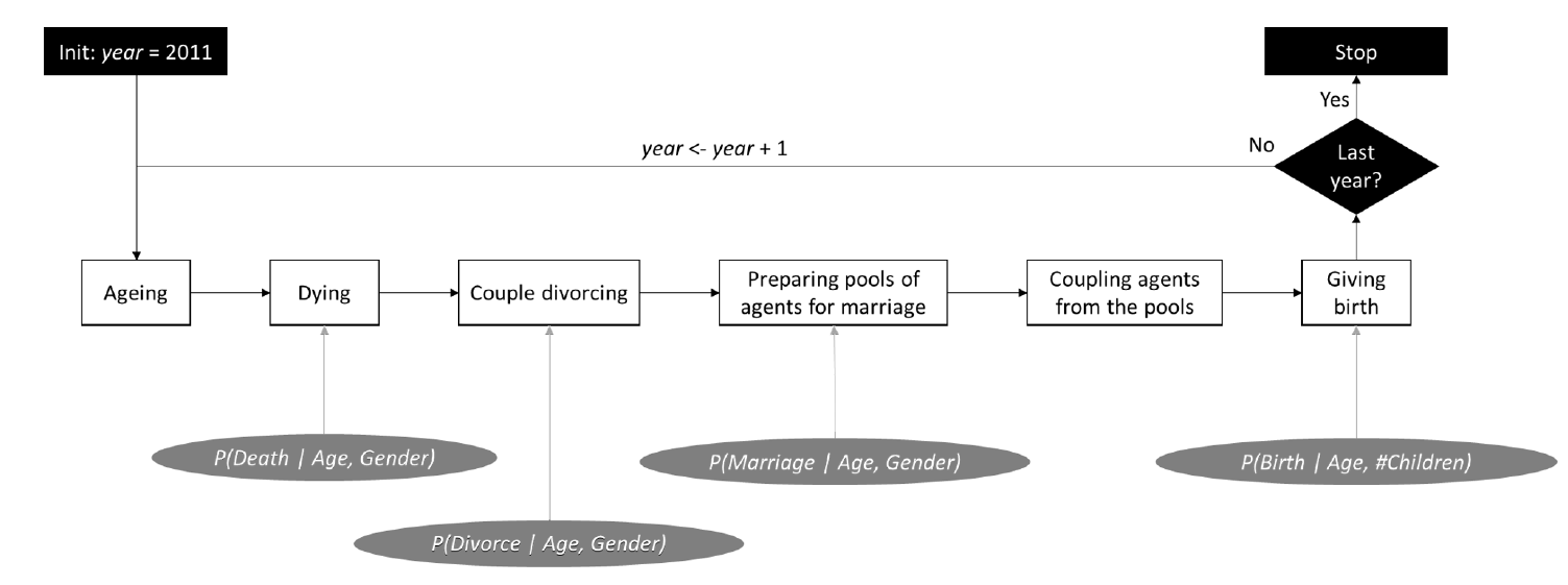
The approach consists of five dynamical processes executed in this specific order: ageing, dying, giving births, divorcing and marrying. It is clear that out of these five processes, only ageing is deterministic (every individual age). On the other hand, the remaining processes are stochastic, i.e., they occur randomly depending on probabilities extracted from available data. Moreover, for death, divorces and marriages, the probability of these events is conditioned by age and gender, while the probability of giving birth is conditioned by the number of previous pregnancies and the age of the female agent. The overall procedure is illustrated in Figure 1. Depending on the event, the structure of the household can be updated. For additional information, these evolution algorithms are fully detailed in Huynh et al. (2013).
For each simulated year, a probability for each possible event is assigned to each synthetic agent. As any other stochastic simulation, these probabilities are then used to determine which events are triggered. As these simulations are not deterministic, several runs could result in slightly different final populations. To control this, a seed can be chosen for the random number generator used by TransMob.
Sensitivity of the Microsimulation
Having introduced TransMob, we now consider different factors that can have a significant impact on the forecasted population. This section contains an overview of the effect of both seed and order on the final simulated population. A preliminary analysis of the influence of these two factors is included in Dumont et al. (2017a). Our aim is to better investigate if the differences in the simulation are due to the order and/or the seed.
As mentioned previously, the order of the models in TransMob was originally predefined (Huynh et al. 2015). Considering that the major aim of this paper is to analyse the impact of an order change, we will first focus on testing each feasible order. It should be noted that simulating birth before ageing implies a double generation of babies, since the initial baseline population already includes 0 year old individuals. Therefore, only orders specifying ageing before birth are considered, resulting thus in 60 feasible orders.
Our analysis also considers the sensitivity of the microsimulation with respect to the choice of the random seeds. Hence we will perform 20 simulations using different seeds for each feasible order[2], resulting in 1,200 experiments simulating 10 years.
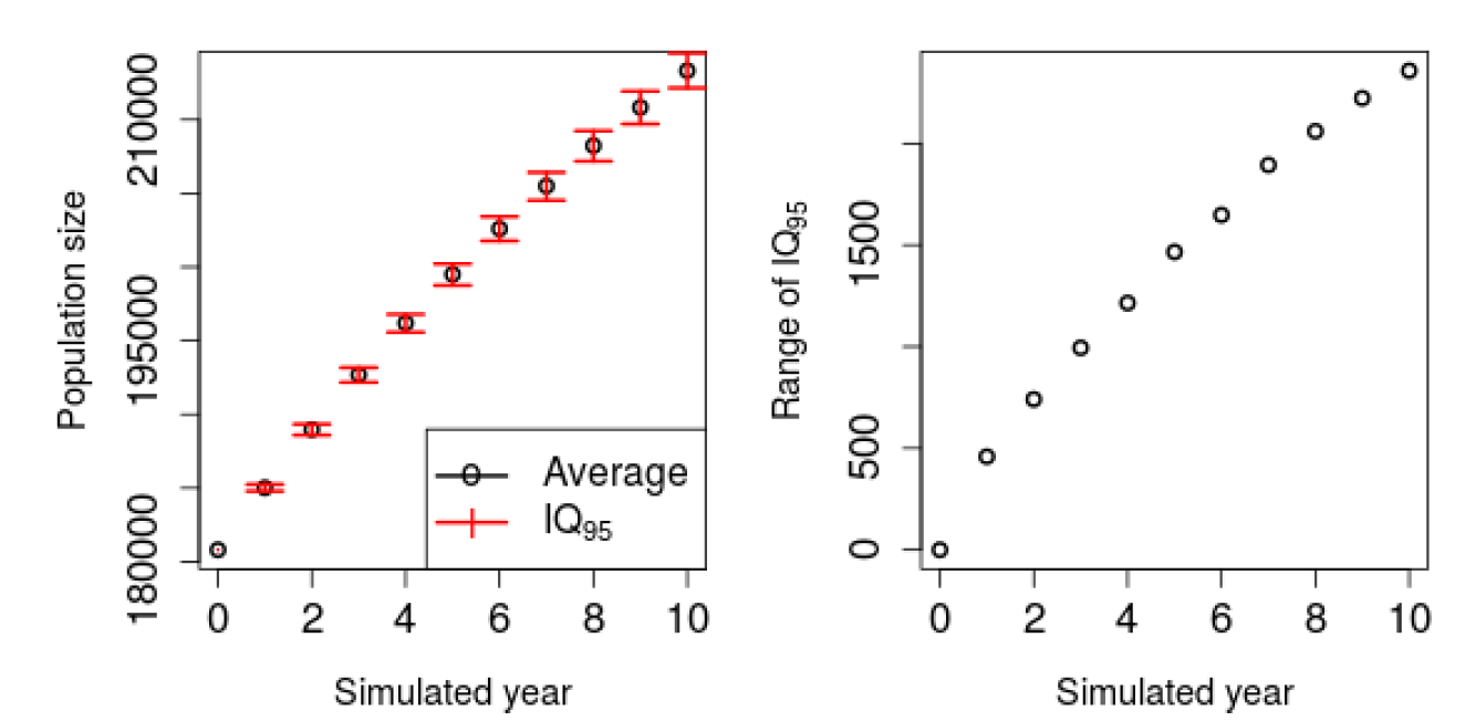
Figure 2 illustrates the average yearly population and the quantile interval IQ95 defined by the 2.5 and 97.5 percentiles (i.e. containing 95% of the simulations). This graph supports the intuition that the difference between several runs increases over the simulated years. We can see that for the last year \(IQ <_{95} = [212,151; 214,509]\) is narrow with the maximum relative deviation between the average and one extremity of the interval being 0.6% of the population.
Impact of the seed
This subsection aims at determining if some random seeds influence the process in a specific direction. For example, one specific seed could systematically results in an older population. Using a statistical analysis based on the well-known ANOVA method (Chambers et al. 1992), Dumont et al. (2017a) concluded the independence between the seed and the retained variables. We hereby confirm this result, see for instance Figure 14 in Appendix A which illustrates that the seed does not influence the final results.
Impact of the order
Does the order in which the procedures are applied influence the tendency of the results? The idea is now to determine if some orders result in a larger/younger population. A preliminary analysis indicates that the order significantly influences results (Dumont et al. 2017a). To identify the differences between the orders, two types of variables need to be introduced:
- indicators of the final population: the number of men, women, as well as the number of individuals in each age class (less than 30 years old, between 31 and 60, and more than 60 years old);
- indicators of the order: the position of each process in the chosen order. For example, if we simulated ageing, then death, then marriage, then birth and finally divorce, the indicators of order are : position of ageing ~=~1; position of death = ~=~2;
For the first set of indicators, the logarithm has been applied for each variable to reduce the impact of exceptionally large populations. By adding these transformations, our results significantly improved.
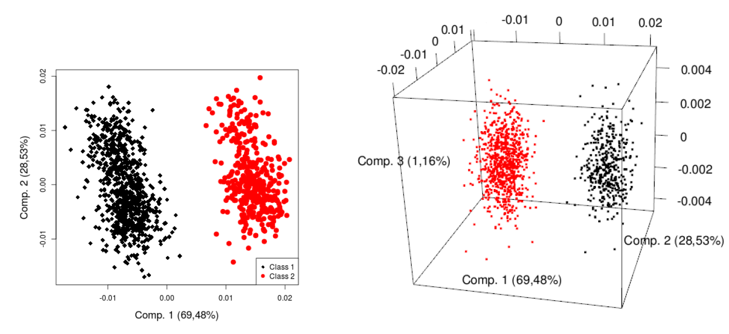
To quantify these differences, a classification is applied on the indicators of the final population. Dumont et al. (2017a) show two distinct classes. Hence, a \(k\)-means classification (Hartigan & Wong 1979) with \(k=2\) followed by a principal component analysis (Wold et al. 1987), or PCA for short, is executed to visualize the different classes. The graphs in 2 and 3 dimensions in Figure 3 confirm the two very distinguishable sets of points. Note that the three first components computed by the PCA already explain 99.18% of the total variance.
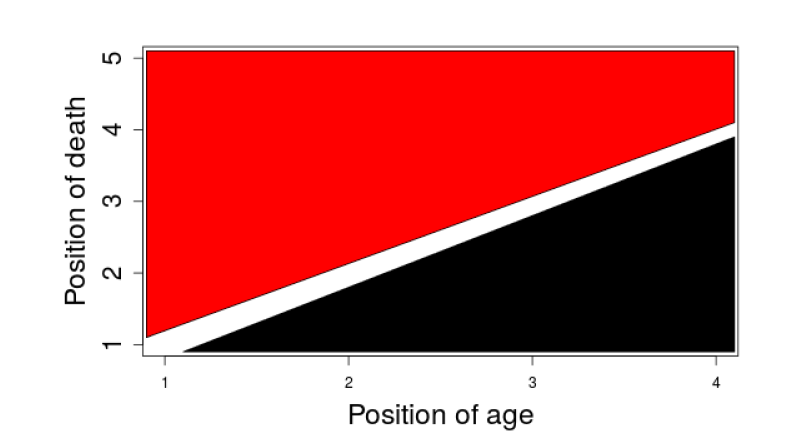
Two well-separated classes can be identified in the results of the simulation. The next step is to identify the discriminant factors for these two classes. We checked that each order over the 20 seeds always lie inside the same class. Thus, only the order categorized simulations. The process to identify patterns for orders belonging to each class was successfully, as shown in Figure 4. Indeed, the position of ageing relatively to the one of death is determinant. When ageing is before death, the simulation ranks into the second class (red) and in the opposite, death before ageing results in the first class (black). Intuitively, this can be explained by the fact that the death probability depends on age. Indeed when ageing, the probability to die increases.
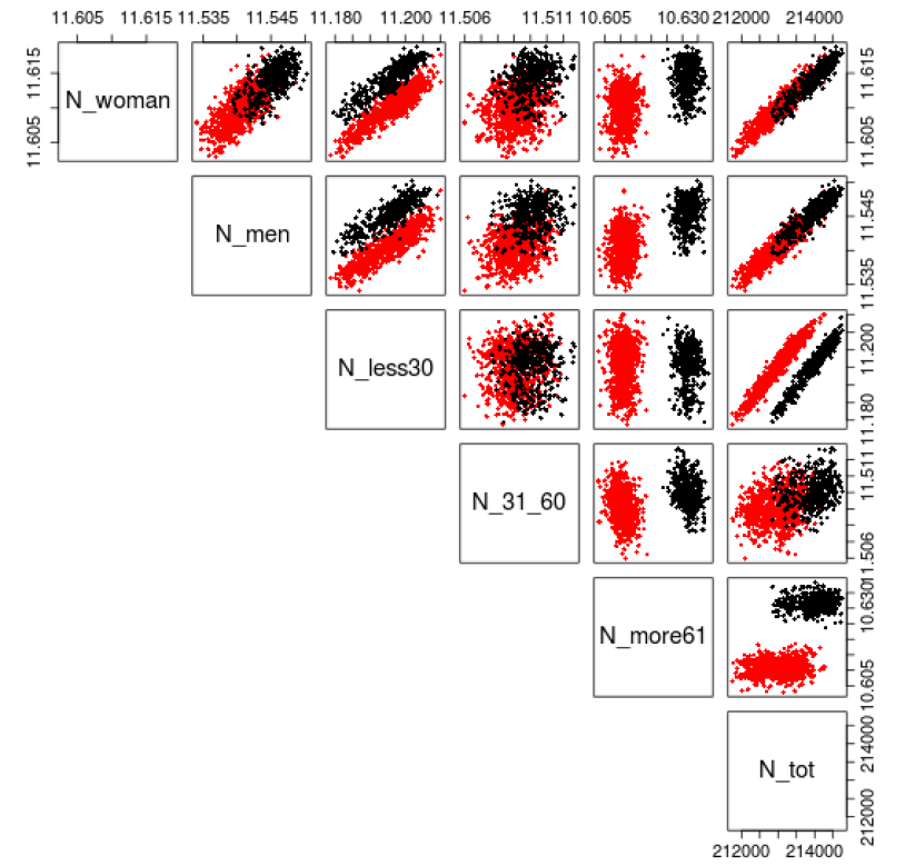
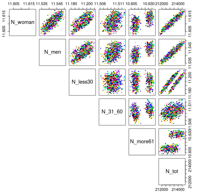
Having the classes established, an analysis of the final populations per class is performed and the results are reported in Figure 5. Two well-separated sets of points clearly appear for each combination of indicators involving the number of individuals being more than 61 years old. On the one hand, the red class stands for all simulations with less elderlies. On the other hand, the black class contains populations with a larger number of elderlies. Moreover, in each graph involving the total number of individuals, we observe that the red dots tend to represent populations smaller than the black ones.
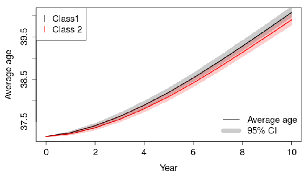
We can also note two almost parallel lines for the combination of the total population and individuals less than 30 years old. This means that by staying on the same class, any increase of the final population implies a constant increase in the number of less than 30 years old persons. However, the two classes are well-separated. This indicates that for two simulations producing the same population size, populations in the red class include more people who are less than 30 years old. Similar conclusions apply when focusing on the number of individuals less than 30 years old per gender, even if this is less prominent. For individuals between 31 and 60 years old, no clear distinction can be made between classes. In summary, the black class contains larger populations with more elderlies and less young people. Note that the average age per class confirms this as shown in Figure 15 in Appendix B.
In summary, the order significantly influences the final population. Indeed, performing ageing before death results in a smaller and younger population.
At this level, the position of the other processes in the dynamical evolution loop does not significantly influence results. The following section proposes a method removing these two events from the possible orders, which enables the analysis of the impact of the order of the three remaining processes.
Reduction of the Number of Possible Orders: A Calendar-Based Approach
Considering that the positions of death and ageing bias the simulation, we decided to propose an alternative method to reduce this impact. By proposing another way to consider ageing and death, the possible remaining orders involve only marriage, divorce and birth, reducing the feasible orders from 60 to 6.
Method
To avoid the high influence of the position of death and ageing, our proposition is to assign a specific date for these events for each synthetic individual. This means assigning a date of death and a birthday for ageing. This technique can be easily extended to other processes as dates could be assigned to every event.
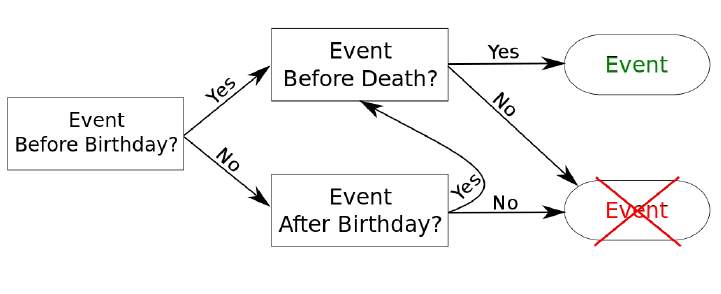
First, the model responsible for death is executed. For each person not dying during this simulated year, the remaining models stay unchanged. However, each individual dying in this year is assigned a date of death and he/she will remain in the population, possibly performing other actions if they arise before his/her death. If an event concerning this agent is planned to happen, we check that this arises before the death. For this, a date is randomly chosen for this event and it is considered only if prior to death.
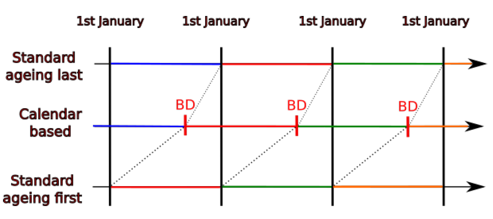
Secondly, a date of birth is also assigned to each individual. Figure 6 illustrates the changes induced by adding this birthday. Colours represent the probabilities of occurrence of a specific event depending on age. We can see that the standard approach with ageing at the end (or at the beginning) considers the age at 1st of January (or 31th December) for the whole civil year, whereas the calendar-based approach adapts the probabilities for each individual at their birthday. While the standard approach implies that probabilities are adapted at the same moment for all individuals, the calendar-based approach permits to change these probabilities depending on each individual's birthday.
It can be noted that the computational cost is different from adopting a time step of one day. Indeed, a daily time step implies considering each process for each individual for each simulated day, whereas our approach still considers each process only once a year for each individual.
The proposed methodology is possible only if we can establish the probability of the event occurring in the year depending on the age of the agent and its birthday.
The naive approach consists in considering that the probability of an event occurring during a civil year can be refined using a convex combination of the probability of the event to happen at the present age and at the age +1. For a person of age \(A\) at the beginning of the year and \(BD\) days from 1st of January to its birthday, the probability of an event \(E\) occurring during the year can be calculated by
| $$P(E)=P(\text{$E$ only before BD }\hspace{0.3cm}\textbf{or}\hspace{0.3cm} \text{$E$ only after BD}) = P(\text{$E$ only before BD })\hspace{0.3cm}\textbf{+}\hspace{0.3cm} P(\text{$E$ only after BD})$$ |
| $$P(\text{$E$ before BD }) = P(\bigcup _{i=1}^{BD}\text{$E$ on day $i$ }) = \sum_{i=1}^{BD} P(\text{$E$ on day $i$ })$$ |
| $$P(\text{$E$ after BD }) = P(\bigcup _{i=BD+1}^{365}\text{$E$ on day $i$}) = \sum_{i=BD+1}^{365} P(\text{$E$ on day $i$ }). $$ |
In this example, we now make the simplifying but unrealistic assumption that \(E\) has the same likelihood to occur any day of the year. Thus, we have[3]
| $$P(\text{$E$ on day $i$}) = P(E|A) * \frac{1}{365}$$ |
| $$P(\text{$E$ on day $i$}) = P(E|A) * \frac{1}{365}$$ |
| $$P(E) = P(E |A)*\frac{BD}{365}+P(E|A+1)*\frac{365-BD}{365}$$. |
It can also be noted that even if we assumed a uniform distribution for the dates, we could easily use any kind of distributions for each model (e.g. an empirical distribution if the data is available).
When considering a uniform distribution of the dates for an event that can arise only once per year (each day has same probability), this can be seen as a sequence of Bernoulli experiments for each day that succeeds if the event happens. The formal analytical determination of this formula gives very similar results to the naive approach developed in this section. The detailed analysis of the formal development is in Appendix D.
A schematic representation of the calendar-based approach is given in Figure 7.
Since we change the procedures for ageing and death, the only remaining possible events are marriage, birth and divorce, leaving only 6 possible orders.
The proposed approach of defining dates for events to avoid problems with possible orders is not limited to ageing and death in population evolution. It can be applied in all fields using these types of agent-based modelling and dates can be generated for each model. We focus here on dates for ageing and death to analyse the impact on the final population since we established above that these two processes strongly influence the size and age of the final population. In our case, divorces are proposed only to couples and marriage only to single individuals. Therefore, these models concern only a part of the population. Even if performing one after the other can slightly modify the set of individuals going through the other model, their impact is limited.
Analysis of the new orders
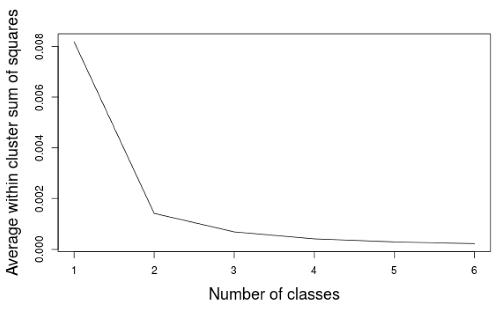
Similarly to the analysis presented in Section 3.6, a classification of the indicators of the final population is also performed using the new improved method. Figure 16 in Appendix C contains the elbow method to determine the number of classes showing an evident elbow at two classes. These two classes are reported on the PCA in Figure 8. The separation of the points is less obvious than for all previous orders. Indeed, no empty space divides the two set of dots. This seems to indicate that the final populations are more homogeneous than previously. However, it is worth analysing the influence of these classes on the final population.
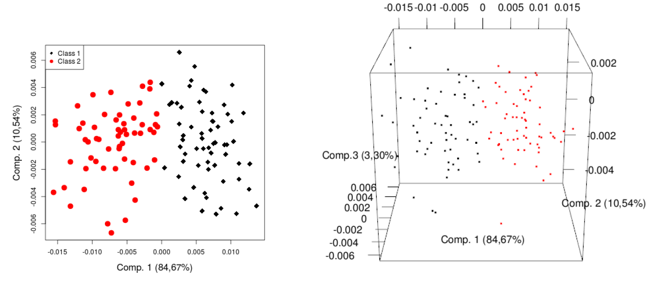
Figure 9 indicates less evident differences between the classes than for the standard method. Nevertheless, the first class (black) has a smaller population composed of less individuals under 30 years old. A slightly linear relation stands between the total population and the number of women, men and individuals less than 30 years old. This means that the larger the total population is, the higher these indicators also are. Yet, the number of individuals older than 31 years old does not follow this linear tendency.
Identifying the patterns in the same classified orders is the next step. A decision tree[4] highlighted the importance of the position of marriage regarding to the birth. Nevertheless, this pattern is less determinant than the one illustrated in Figure 4.

The relation between marriage and birth is very important in the model, since only married women can give birth (see Huynh et al. 2015 for more details on models and Huynh et al. 2016 for the definition of "married" women, which also includes de facto relationships).
Table 1 presents the number of simulations in each class for each order in more details. One can appreciate from the latter Table that any given order can belong to both classes, even though there a clear tendency for one of the class. This indicates that the seed has now a larger impact than previously and supports the observation about the homogeneity of the final populations.
| First Model | Second Model | Third Model | #Simulations in Class 1 | #Simulations in Class2 |
| Marriage | Divorce | Birth | 16 | 4 |
| Marriage | Birth | Divorce | 20 | 0 |
| Divorce | Marriage | Birth | 19 | 1 |
| Divorce | Birth | Marriage | 0 | 20 |
| Birth | Divorce | Marriage | 1 | 19 |
| Birth | Marriage | Divorce | 2 | 18 |
Comparison
In this section, we compare the performance of the calendar-based approach against the classical one. The main purpose of the new method is to reduce the variability of the final populations. For the comparison, the final population indicators after 10 years are computed for 20 random seeds and for all feasible orders with and without the introduction of dates of birth and death.
The homoscedasticity of the total population indicator over the two groups with and without dates is tested. Note that the group with calendar-based includes 120 simulations (6 orders and 20 seeds), whereas the other group includes 1200 simulations (60 orders and 20 seeds). Due to the imbalance and small size of groups, a careful choice of the method to test homoscedasticity is required. Parra-Frutos (2013) analysed different statistical tests and concluded that in unbalanced and small samples, the best ways to test homogeneity of variance includes the James test, the Welch test and the Alexander and Govern test. Dag et al. (2017) incorporated these tests in a package for the R programming language (R Core Team 2018). The three tests allow to conclude the non homogeneity of the variances with a confidence level of 0.95. The standard deviations are 645.05 for the classical simulations and 529 for the simulations using dates. This indicates that the proposed method reduces the variance between runs.
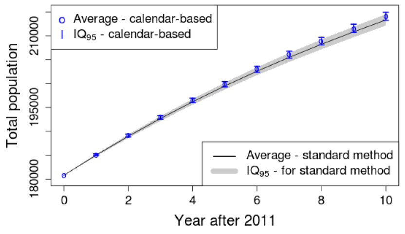
Figure 10 shows the average population and the IQ95 interval per year and per type of simulation. Note the difference both in variances and averages. Addings dates produces sensibly larger populations on average, overlapping the top half of the IQ95 of standard simulations.
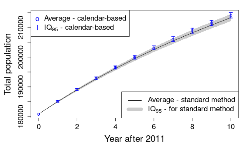
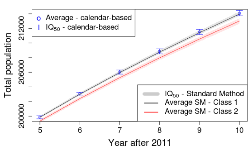
As previously mentioned, standard simulations are typically classified in two groups depending on the final population size. Here, it is important to verify if calendar-based simulations match the class associated with the largest final populations generated by the standard approach. Figure 11 focuses on the 5 last simulated years and shows the IQ50.
Results show that the calendar-based approach produces final populations similar to the ones in the first class in terms of total population. Performing again the tests suggested by Parra-Frutos (2013) to examine the homogeneity of variance, we found that for the three tests that variances inside the first class and the simulations using dates are not significantly different.
Here, it is interesting to compare the distributions. As the assumptions for the classical ANOVA test are not met, we used the non-parametric Kruskal-Wallis test. The p-value of 0.47 indicates that no distribution stochastically dominates the other. This confirmed that the relative difference between the average of the two groups is only 0.03%.
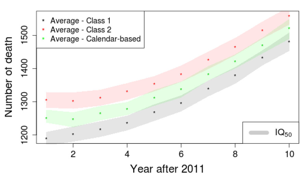
Considering that the size of the populations produced by the calendar-based approach and the first class of standard methods were statistically similar, we then looked at the structure of the different populations. Indeed, the population size could be equal while their age structure differs. This is illustrated in Figures 12 and 13 where death and birth evolutions are displayed. Unlike expectations induced by Figure11, Figure 12 shows that the calendar-based approach produces a number of deaths in between the ones generated by the two classes of standard methods. This indicates that the proposed approach actually produces populations that are different from the ones belonging to the first class. The evolution of the numbers of births in Figure 13 shows a different picture. Indeed, the calendar-based approach generates a larger number of births compared to the others two methods.

This explains why the calendar-based approach and the first class of standard methods generate populations of similar sizes. Therefore, it is possible to argue that the proposed calendar-based methodology is the most appropriate approach.

Conclusion and Discussion
After investigating all the feasible orderings of models and presenting a promising calendar-based approach, we believe that our work made two contributions to the field of agent-based models for demographic evolutions that could be extended to other agent-based models.
First, this work showed the importance of the order of the models in agent-based modelling, after having checked the stability against random seeds. For TransMob, including five major processes, i.e., ageing, death, birth, marriage and divorce, we highlighted significant differences in the results of the simulation if death is performed after or before ageing.
Secondly, we proposed to assign dates to key events and redefine the probabilities depending on these dates. We found that this method decreased the variability of the simulations. Furthermore, this is not restricted to the evolution of synthetic populations. Indeed, for each process interfering with probabilities of other model, we can assign a date for this event (either from a uniform distribution amongst the days of the year or from a defined distribution if you for example have the prevalence of birth per day in the year). Thanks to this date, probabilities of dependent events can be adapted with a weighted linear combination of the probabilities before and after the determinant event.
The code associated to the calendar-based approach is available at the following address: https://github.com/smart-facility/calendar-based-microsim
The proposed method allows simultaneously to avoid any bias induced by choosing a specific order, reduce the variability of the results and approximate a daily time step with a reduced computational cost.
This work allows us to propose certain guidelines for future agent-based models (with a discrete time step). Indeed, for one iteration of the evolution loop, we propose the following flow:
- Processes implying to remove agents are evaluated to identify the agents that will disappear. However, these agents are not removed directly. Instead, a date of removal of the agent is determined.
- Processes changing agent characteristics influencing the probabilities of other processes are executed and dated. For individuals disappearing this iteration, we check if each event is before or after the removal date.
- Remaining processes are launched with updated probabilities. For individuals disappearing this iteration, we check if each event is before or after the removal date.
- Agents disappearing during this iteration are removed.
It should be noted that this is a general proposition limiting the influence of the order. Unfortunately, some questions are still unsolved. For instance, if processes are interdependent or if we have several processes in third step, several orders are still possible.
Obviously, the proposed approach has certain limitations. For instance, there is need for additional data if one wants to draw dates from a realistic distribution through the year and events are unpredictable. The practitioner should also be aware that all these agent-based simulations are always highly dependent to the type and quality of input data (garbage in-garbage out process). Finally, it should also be noted that this does not necessarily allow to extend the time horizon of good predictions.
In future works, a more generalised analysis could be performed, considering additional (fictive) models with probabilities generated randomly with respect to constrains such as dependencies with agent characteristics and/or interdependencies with other modules and/or orders between modules. Any generalisation to agent-based models is a big challenge, since each case is different and generating a population kangaroos in Australia cannot be similar to simulating particles in an accelerator or examining demographic evolution.
Acknowledgements
This research is part of a project with the support and funding of the Public Service of Wallonia (DGO6), under Grant No. 1318077. Computational resources have been provided by the Consortium des Équipements de Calcul Intensif (CÉCI), funded by the Fonds de la Recherche Scientifique de Belgique (F.R.S.-FNRS) under Grant No. 2.5020.11. Finally, we gratefully acknowledge the support of NVIDIA Corporation with the donation of the Titan Xp GPU used for this research.Notes
- TransMob contains different modules, each one composed of different models.
- Indeed launching the process several times with the same seed will always produce the same results.
- This also assumes \(P(E\) on day \(i\) and not on another day)=\(P(E\) on day \(i\)).
- Obtained using the package in Therneau et al. (2017).
Appendix
A: Uncertainty - Influence of seed
B: Average age of the population per class
C: Number of classes of orders when dates are added
Appendix D: Formal establishment of the new probabilities
The aim of this appendix is to establish formally the probability of an event \(E\) during a civil year depending on the age A of the agent at the beginning of the year and its birthday happening a day \(BD\).
Rather than directly computing this probability, the first step consists in considering the complementary probability of the event, i.e. the probability that the event is not happening during the year. This can be expressed as the probability that the event is not happening in any day during the year. Let us denote by \(E_i\) the event \(E\) occuring on day \(i \in \{1,\dots,365\}\). If we assume the conditional independence between the \(E_i\), we have:
| $$\begin{eqnarray*}P(E~|~A,BD)& =& 1 - P(\neg E~|~A,BD) \nonumber \\ & = & 1 - P(\bigcap_{i=1}^{365}\neg E_{i} ~|~A,BD) \nonumber \\ & = & 1 - \prod_{i=1}^{BD} P(\neg E_{i}~|~A)\prod_{i=BD+1}^{365} P(\neg E_{i}~|~A+1) \nonumber \\ & = & 1 - \prod_{i=1}^{BD} (1 - P(E_{i}~|~A))\prod_{i=BD+1}^{365} (1 - P(E_{i}~|~A+1)) \nonumber \\\end{eqnarray*}$$ |
This general expression holds for any distribution of the independent events \(E_i\). In our context, we make the additional assumption that the events in the set \(\{E_i ~ | ~ i = 1,\dots,BD\}\) are identically distributed, as well as the events in the set \(\{ E_j ~ | ~ j = BD+1,\dots,365 \}\). Thus we can write:
| $$\begin{eqnarray*}P(E~|~A,BD) & = & 1 - \prod_{i=1}^{BD} ( 1 - P(E_{BD}~|~A) ) \prod_{i=BD+1}^{365} ( 1 - P(E_{365} ~ |~A+1) )\\ & = & 1 - (1 - P(E_{BD}~|~A))^{BD} (1 - P(E_{365}~|~A+1))^{365-BD} \\ \end{eqnarray*}$$ |
Using a similar reasoning, the probability \(P(E_{BD}|A)\) can now be derived thanks to the probability \(P(E~|~A)\) provided in the input tables and using the fact that the \(E_i\) are independent and identically distributed. Indeed, we have:
| $$\begin{eqnarray*}P(E~|~A)& =& 1 - P(\neg E ~| ~ A) \nonumber \\ & = & 1 - P(\bigcap_{i=1}^{365}\neg E_i ~| ~ A) \nonumber \\ & = & 1 - \prod_{i=1}^{365} P(\neg E_i ~ | ~ A) \nonumber \\ & = & 1 - \prod_{i=1}^{365} (1 - P(E_i ~|~A)) \nonumber \\ & = & 1 - \prod_{i=1}^{365} (1 - P(E_{i}~|~A)) \nonumber \\ & = & 1 - (1 - P(E_{i} ~ |~ A))^{365} \nonumber \\\end{eqnarray*}$$ |
Isolating the probability for a specific day \(P(E_i ~| ~ A)\), we obtain:
| $$\begin{eqnarray*}(1 - P(E_{i}~|~A))^{365} & = & 1 - P(E~|~A) \nonumber \\ 1 - P(E_{i}~|~A) & = & \sqrt[365]{1 - P(E~|~A)}\\ P(E_{i}~|~A)& = & 1- \sqrt[365]{1 - P(E~|~A)}\end{eqnarray*} $$ |
As the \(P(E_j ~| ~ A + 1)\) can be obtained in a similar way, we now have all the elements to be able to generate the probabilities \(P(E~|~A, BD)\) required by the model. It should be noted that results mimic the ones of the naive method as we can see in Figures 17 and 18.
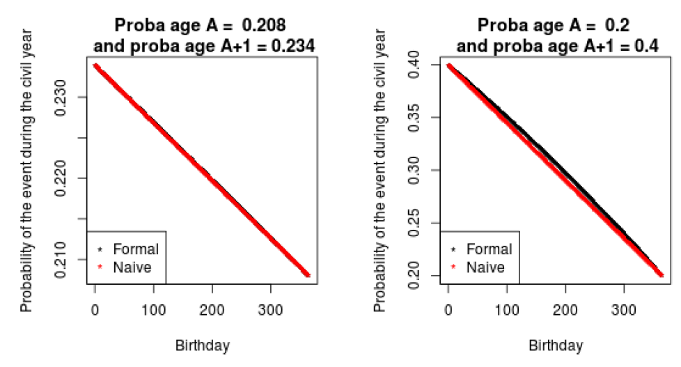
To illustrate the relation between the exact and naive probabilities depending on the birthday, two examples have been plotted in Figure 19. The differences are almost indistinguishable on the le panel representing probabilities of having a first baby at the ages of 25 and 26. On the right, a second test takes into account probabilities more affected by the change in age (difference of 20%). The difference is noticeable for the birthday on the middle of the year, but the two methods stay really close to each other. For this reason, the naive approach can be considered, since it is easier and gives similar results.
References
BARTHÉLEMY, J. (2014). A parallelized micro-simulation platform for population and mobility behaviour - Application to Belgium. Ph.D. thesis, University of Namur.
BARTHÉLEMY, J. & Toint, P. L. (2013). Synthetic population generation without a sample. Transportation Science, 47(2), 266–279.
BECKMAN, R. J., Baggerly, K. A. & McKay, M. D. (1996). Creating synthetic baseline populations. Transportation Research Part A: Policy and Practice, 30(6), 415–429. [doi:10.1016/0965-8564(96)00004-3]
CHAMBERS, J. M., Freeny, A. & Heiberger, R. M. (1992). 'Analysis of variance: Designed experiments.' In J. M. Chambers & T. J. Hastie (Eds.), Statistical Models in S, Wadsworth: Brooks/Cole.
CORNELIS, E., Barthelemy, J., Pauly, X. & Walle, F. (2012). Modélisation de la mobilité résidentielle en vue d’une micro-simulation des évolutions de population. Les Cahiers Scientifiques du Transport, 62, 65–84.
DAG, O., Dolgun, A. & Konar, N. M. (2017). Onewaytests: One-Way Tests in Independent Groups Designs. R package version 1.5: https://CRAN.R-project.org/package=onewaytests.
DUMONT, M., Barthelemy, J., Carletti, T. & Huynh, N. (2017a). Importance of the order of the modules in TransMob. Proceedings of MODSIM2017.
DUMONT, M., Carletti, T. & Cornélis, É. (2017b). Vieillissement et entraide: Quelles méthodes pour décrire et mesurer les enjeux?. Univer’Cité, 6, 55.
GARGIULO, F., Ternes, S., Huet, S. & Deffuant, G. (2010). An iterative approach for generating statistically realistic populations of households. PloS one, 5(1), e8828. [doi:10.1371/journal.pone.0008828]
HARTIGAN, J. A. & Wong, M. A. (1979). Algorithm AS 136: A k-means clustering algorithm. Journal of the Royal Statistical Society. Series C (Applied Statistics),28(1), 100–108.
HUYNH, N., Barthelemy, J. & Perez, P. (2016). A heuristic combinatorial optimisation approach to synthesising a population for agent based modelling purposes. Journal of Artificial Societies and Social Simulation, 19(4), 11: https://www.jasss.org/19/4/11.html. [doi:10.18564/jasss.3198]
HUYNH, N., Namazi-Rad, M.-R., Perez, P., Berryman, M., Chen, Q. & Barthelemy, J. (2013). Generating a synthetic population in support of agent-based modeling of transportation in Sydney. 20th International Congress on Modelling and Simulation (MODSIM 2013) (pp. 1357-1363). Australia: The Modelling and Simulation Society of Australia and New Zealand.
HUYNH, N., Perez, P., Berryman, M. & Barthélemy, J. (2015). Simulating transport and land use interdependencies for strategic urban planning - An agent based modelling approach. Systems, 3(4), 177–210. [doi:10.3390/systems3040177]
LENORMAND, M. & Deffuant, G. (2012). Generating a synthetic population of individuals in households: Sample-free vs sample-based methods. arXiv preprint arXiv:1208.6403.
LOVELACE, R. & Dumont, M. (2016). Spatial Microsimulation with R. CRC Press. [doi:10.1201/b20666]
MILLER, E. J., Hunt, J. D., Abraham, J. E. & Salvini, P. A. (2004). Microsimulating urban systems. Computers, environment and urban systems, 28(1), 9–44.
PARRA-FRUTOS, I. (2013). Testing homogeneity of variances with unequal sample sizes. Computational Statistics, 28(3), 1269–1297. [doi:10.1007/s00180-012-0353-x]
R CORE TEAM (2018). R: A Language and Environment for Statistical Computing. R Foundation for Statistical Computing, Vienna, Austria: https://www.R-project.org/.
THERNEAU, T., Atkinson, B. & Ripley, B. (2017). rpart: Recursive Partitioning and Regression Trees. R package version 4.1-11: https://CRAN.R-project.org/package=rpart.
WOLD, S., Esbensen, K. & Geladi, P. (1987). Principal component analysis. Chemometrics and Intelligent Laboratory Systems, 2 (1-3), 37–52.
YE, P., Hu, X., Yuan, Y. & Wang, F.-Y. (2017). Population synthesis based on joint distribution inference without disaggregate samples. Journal of Artificial Societies and Social Simulation, 20(4), 16: https://www.jasss.org/20/4/16.html. [doi:10.18564/jasss.3533]