
Introduction
From the supply-side perspective, the development of each sector or industry is a complex and long-lasting process, affected by numerous factors of different origin. In the case of agriculture and agro-food production, the predominant role is played by factors associated with local weather and soil conditions, technological advances, tradition and experience in plant cultivation and their processing, knowledge exchange, applicable legal regulations, the existing system of subsidies or support programmes, conditioned by current and expected demand. Wine industry is a specific sub-sector of agribusiness and is strongly influenced by behavioural factors of a social nature (e.g. group membership, networking), personal nature (e.g. lifestyle, status) or psychological nature (e.g. motivations, perception). Thus, its development is determined by the coexistence of both profit- and utility-driven market agents (Scott Morton & Podolny 2002).
The impact of behavioural factors is particularly evident in emerging markets such as Poland, with unfavourable climatic and legal conditions and a past deeply marked by recurrent political and economic upheavals (military aggression, the communist regime), where running one's own vineyard seems more akin to a hobby than an economically rational activity. Nevertheless, as revealed by official statistics from the Polish Agricultural Market Agency (ARR), the number of registered wine producers and the area under cultivation has been consistently growing at a strong rate over recent years (Table 1). These figures are, in practice, much greater when taking into account all of the unregistered small farmers and home gardeners (only the large professional producers are obliged to register). The Małopolska voivodship, located in the southern part of Poland, contains the oldest wine-growing regions, with the origins of viticulture dating back to the 9th century AD. .
As the domestic wine market is presently undergoing dynamic development (restoration), questions of particular importance are those concerning the possible directions and major determinants of its industrial organization, the dynamics of vineyard creation and the spatial relationships governing vineyard location. It may be perceived as a kind of trend or innovation in domestic agribusiness that is spreading across the regions, including Małopolska.
| Production year | 2009 | 2010 | 2011 | 2012 | 2013 | 2014 | 2015 | 2016 | 2016/09 |
| Number of producers | 21 | 20 | 26 | 35 | 49 | 76 | 101 | 151 | 719% |
| Total area (ha) | 36.05 | 37.01 | 58.6 | 97.88 | 99.49 | 134.35 | 194.24 | 221.26 | 614% |
| Wine production (hl) | 412.5 | 437.10 | 428.5 | 898.2 | 1978.9 | 3392.0 | 5017.3 | 6993.8 | 1696% |
| Area per producer (ha) | 1.72 | 1.85 | 2.25 | 2.80 | 2.03 | 1.77 | 1.92 | 1.47 | 85% |
| Production per producer (hl) | 19.64 | 21.86 | 16.48 | 25.66 | 40.39 | 44.63 | 49.68 | 46.32 | 236% |
The objective of this paper is to develop an agent-based model allowing us to understand the way different factors influence supply-side diffusion in a wine industry with objective environmental constraints. An additional goal is to assess the predictive power of the created model and compare it to a standard econometric model. Here, we showed that the agent-based model possesses good explanatory power and provides a significant micro-level insight into the important factors driving viticulture development in the Małopolska region. Thus, we conclude that in this scenario an agent-based approach is to be preferred both qualitatively and quantitatively to econometric modelling.
Characteristics of Polish Vineyard Market
The Polish wine market is dominated by relatively small vineyards, with an average area of 1.47 ha according to ARR data. The drop in the cultivated area per producer, which is evident over the analysed period, confirms the growing presence of small entities in the market. In parallel, the increase in unit production levels may be a testament to the pronounced professionalism and productivity enhancement in the wine industry itself. These observations correspond to survey results which supplement our data set containing official statistics. The survey was conducted among vineyard owners from Małopolska voivodship and allowed us to discern the main motives underlying owners' decisions to establish and operate a vineyard and to verify their orientation toward either utility maximisation or profit maximisation. The survey was conducted electronically and on paper. The winemakers were approached through wine organizations, and we received 22 surveys (18 surveys were fully completed). Due to the high degree of land fragmentation in this region, where 34.5% of all farms cultivate an area of approximately 1-2 ha and 82.3% cultivate less than 5 ha of agricultural land (Stachanczyk & Tutaj 2016), we divided all vineyards into small (S) and large (L) entities, selecting the area of 0.5 ha as the differentiating parameter (the vineyards with an area smaller than 0.5 were classified as small; the others were classified as large). The main results of the survey are shown in Table 2. The small and large vineyard owners differ in business purposes, motivation and inclinations to associate with one another and their sources of knowledge concerning wine growing and production.
The behaviour and attitudes of owners differ between both groups of wine makers. For example, 57% of respondents owning small vineyards indicated that the process of vine cultivation and wine making is an essentially non-profit activity associated with leisure or a hobby. None of them treated it as their primary source of income (see Kolasa 2017 for a recent study of income distribution in Poland). Furthermore, they attached greater importance to knowledge sharing (average factor strength: 9.67 points in an ascending 10-point scale) and acquiring information on wine growing from books or research papers (9.17 points). In contrary, for 25% of the large vineyards, vine cultivation and wine making was a revenue-generating core business and for a further 31% it represented a side-line, complementary to other commercial or agricultural activities. Moreover, 43% of large vineyards tend to be established on plots acquired intentionally for viticulture purposes by investors with an explicit profit motive. Membership in more than one industry association (1.25, on average) would appear to have constituted a means of building their position (and prestige) in the market and sharing knowledge with fellow professionals.
We gathered the following data points in the survey: the area represents the surface area of the vineyard in ha., and the membership in associations gives the number of wine associations the participant is associated with. We also asked for motivations/perceptions in the form of closed yes/no questions (coded as binary variables). In particular, the intentional purchase of land variable assumes the value 1 if the land has been purchased (leased) specifically for viticulture, the main business activity variable is taken to be 1 if running a vineyard is the main activity (taking different sources of income into consideration), and the non-profit activity have the value 1 if there is no economic motivation behind running the vineyard. For other questions concerning the importance of different factors, the participants could choose any integer number from the range 1 to 10, with 1 meaning not at all important and 10 meaning very important. In particular, the survey participants were asked how important for them were the following motivations: enotouristic (wine tourism), hobby/entertainment, prestige in establishing a vineyard, and how important is literature and knowledge sharing. For each variable, in order to evaluate the statistical significance of the differences between groups of small and large vineyard owners, we compared the means using one-sided (less or greater) t test reporting t statistic (value) and respective significance level (p.value). The observed dissimilarities between the two groups of wine market participants render it justifiable to consider small vineyards to be more like utility maximisers and large vineyards function more as profit maximisers. Due to the limited sample size we did not directly use these results for parametrisation of the ABM model. However, the results of the survey allowed us to distinguish two groups of wine producers: small and large in the model.
| category | variable | mean small | mean large | alternative | value | p-value |
| business | area | 0.23 | 1.50 | less | -2.45 | 0.02 |
| business | intentional purchase of land | 0.08 | 0.43 | less | -1.58 | 0.08 |
| business | main business activity | 0.00 | 0.25 | less | -1.53 | 0.09 |
| business | non-profit activity | 0.57 | 0.25 | greater | 1.50 | 0.08 |
| motivation | enotouristic | 4.50 | 6.86 | less | -1.36 | 0.10 |
| motivation | hobby | 9.17 | 6.71 | greater | 1.87 | 0.05 |
| motivation | prestige | 4.08 | 6.14 | less | -1.58 | 0.07 |
| associations | membership in associations | 0.79 | 1.25 | less | -1.41 | 0.09 |
| knowledge | literature | 9.17 | 6.83 | greater | 2.74 | 0.01 |
| knowledge | knowledge sharing | 9.67 | 7.67 | greater | 1.64 | 0.08 |
Related Literature
The question concerning how different factors affect viticulture and wine industry development is one of the major research topics in wine economics. The complexity underlying such factors justifies grouping them into two general subsets: environmental factors and human-dependent factors, which are naturally in mutual interaction.
The role and the climatic impact, land characteristics and seasonal weather conditions on grape and wine production, quality or prices are well known and have been examined in many studies (Gergaud & Ginsburgh 2008; Chevet et al. 2011; Ashenfelter & Storchmann 2010b, 2016; Schultz 2016). The majority of studies point to temperature, precipitation, humidity and insolation as the most significant environmental factors determining grape harvest size and grape quality (Bardaji & Iraizoz 2015; Ashenfelter & Storchmann 2010a). These factors vary between regions, thus differentiating the regional or local potential for industry development. Ongoing climate change and global warming have had a particularly evident influence on viticulture (De Salvo et al. 2014; van Leeuwen & Darriet 2016; Tóth & Végvári 2016). These processes pose a challenge to traditional wine regions and induce shifts in the geographical distribution of wine entities worldwide by giving impetus to emerging wine countries with hitherto less conducive climate conditions, such as, for instance, Canada (Shaw 2017), Denmark (Bentzen et al. 2009), Poland (Czupryna & Oleksy 2014) or Sweden (Rytkönen 2013).
The geographical concentration of favourable environmental settings stimulates human behaviour or activities of varying types and character. Firstly, the wine growing sector attracts individuals (entrepreneurs) with socially- and emotionally-driven attitudes toward business, who attach great importance to utility maximisation objectives. The wine quality (high or low) may possibly differentiate profit- and utility-oriented owners (Scott Morton & Podolny 2002). The phenomenon of conspicuous production, putting emphasis on the wealth and social status of the winery owner is one example of such behavioural inclination (Overton & Banks 2015).
Secondly, the incidence of networking, based on cooperation among wine growers, acts as a fundamental driving force for industry diffusion, especially in a clustered environment (Doloreux & Lord-Tarte 2012; Giuliani 2013; Li et al. 2015). It enables knowledge sharing (Giuliani & Bell 2005; McIntyre et al. 2013) and creates space for undertaking joint marketing or sales initiatives, often aimed at gaining international repute (Dalmoro 2013). As revealed by Belich (2009), this may be even more important to achieve economic dominance than innovation. Nevertheless, close and sustainable collaboration between trade networks and scientific organisations leads to greater competitiveness of inter-connected business entities, which is particularly evident in the Old World wine producing countries (Cassi et al. 2012). A popular and effective way of networking takes place through membership in industrial associations and professional organisations (Corby 2010; Schmitt 2015).
Thirdly, legal regulations and industry standards establish a framework for potential development of the sector and determine market organisation, both at a macro and micro level. In countries with a long tradition in wine making, patronage principles tend to be employed to support the national and regional heritage of wine production and to preserve the distinctive local character of wine products (Gade 2004). The organizational features of farm wineries (e.g., the size and ownership of vineyard acreage, the number of brands or advertising intensity) impact the winery mortality rates and enable changes in industry concentration to be explained by distinguishing two strategic organisational sub-populations: generalists and specialists (Swaminathan & Delacroix 1991; Swaminathan 2001).
The number and variety of both environmental and human factors influencing wine industry development is in fact much broader. Thus, the extrapolation of this process justifies the use of simulation models based on agent interactions in a predefined and simplified setting. Agent-based modelling is perceived as an important analysis framework in social sciences (Farmer & Foley 2009) since it permits the modelling of agents’ heterogeneity and the emergence of self-organisation (Macal & North 2010). It also finds widespread use in agricultural sector analyses and simulations. The mainstream literature in this field examines the impact of agricultural policies on rural environmental management and farmers' behaviour (Brady et al. 2012; Lobianco & Esposti 2010; Berger et al. 2006). Numerous studies confirm that multi-agent models are a powerful approach for analysing spatial diffusion of innovations and resource use changes in agriculture (Berger 2001), as well as explaining interaction between firms in agro-food supply chains and networks (Ross & Westgren 2009).
For example, in the context of what is referred to as "co-opetition" (the hybrid of competition and cooperation) and innovation diffusion Garcia & Atkin (2007) examined the influence of screwcaps on fine wines (a kind of resistant innovation) on consumer behaviour and on wineries strategies. Bouzdine-Chameeva & Galam (2011) examined the impact of wine quality assessment on the dynamics of consumers wine purchasing behaviour and proposed a model based on social interactions among consumers, allowing wine producers to increase the number of loyal clients. Tissot et al. (2014) in their prototype model simulate the impact of climate changes on wine growers' activities and their production strategies. Delay et al. (2015) analysed the influence of cooperative organisation of wine growers operating in mountainous areas on socio-economic and landscape developments in the wine-growing region.
The process of innovation diffusion has been the subject of intensive research, not only in the context of agriculture but in other fields. Bass (1969) applied a differential equation model with a coefficient of innovation and imitation to explain innovation process dynamics. The diffusion model has been extended with respect to perception, learning, preference structure and adoption decision rule in various ways, see Mahajan et al. (1991). An agent-based (bottom-up) approach, which focuses on modelling individual decisions and enables taking heterogeneity and social structures into consideration, has also been widely used to study the process of innovation diffusion. For an overview of this, see Kiesling et al. (2012). They classify existing models depending on a model of consumer adoption behaviour (simple decision rules, utilitarian, state transition, opinion dynamics, and social psychology approaches among others), and modelling of social influence (levels of social influence, interaction topologies and qualitative modelling of social influence). Similarly, Groeneveld et al. (2017) classify the approach to decision-making in land-use models in the following three categories: heuristics, stochastic component and optimisation.
This approach goes back to cellular automata models (Conway 1970; Schelling 1971), and has a long tradition in the literature. The modelling approach is simpler but more abstract (compared to heuristics or optimization approaches) and requires less input. For example, Janssen & Ostrom (2006) suggested relatively uncomplicated models with simple reactive agents when many agents are being considered and the goal is to provide explanations for the observed data, whereas heuristics and optimisation approaches are used to generalise the laboratory experiments or survey data. An optimisation approach was for instance, applied by Krebs (2017). The model requires specification of the partial preference functions and the trade-off weights among them. The classification and preferences parameters for the five types of agents under consideration use heuristics and are derived from Need For Closure scale. The complexity and the data required in the optimisation approach-based land use models is discussed in the following paragraph.
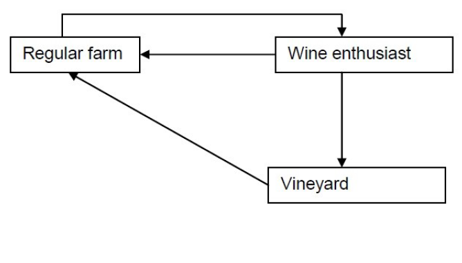
As we consider many agents (all farms in Małopolska) and the data available is limited (e.g. we have survey data but only from the vineyard owners. Additionally, the limited number of surveys enabled us to find only some of the differences between small and large vineyards but not to isolate other homogeneous groups). We therefore decided to use a rather simple model that focuses on spatial relationships and not on the decision process. We considered large and small farms (vineyards). We did not explicitly model profit- and utility-maximisation processes, although one may interpret large vineyards as more profit-driven and small vineyards as more utility-driven. Therefore, we used the state transition (stochastic component) approach, representing the decision process as a transition between the following three states (for example, Goldenberg et al. 2007 and Thiriot & Kant 2008 also use more than two agent states): regular farms, wine enthusiasts and vineyard owners. Using three agent states allowed us to decompose innovation diffusion into two processes; the proliferation of wine enthusiasm (having a more social component) and the establishment of a vineyard (having a more individual component). These two processes may be governed by different parameters.
The presence of vineyards in the neighbouring communities may have positively influenced the spread of wine enthusiasm (discussions, visits, wine tasting) but negatively influence the decision to establish a vineyard (increased competition in a local market). We also factored in a meso-level social influence, Kiesling et al. (2012), as the immediate social environment (the same community or neighbouring ones) influences the transition probabilities. This influence may also be micro-funded by bilateral contacts, as in word-of-mouth approach, see e.g. Arndt (1967), Mahajan et al. (1991), and Kowalska-Styczeń & Sznajd-Weron (2016). The meso-level approach does not require modelling of the social network structure or bilateral contacts.
Matthews et al. (2007) reviewed the agent based land use models and classified existing models with respect to their purpose: policy analysis and planning, participatory modelling, testing hypotheses of land-use and settlement patterns, testing social and economic science concepts, and modelling landscape function. Filatova et al. (2013) also surveyed the existing literature of spatial agent-based models applied to socio-ecological systems. Lobianco & Esposti (2010) proposed a Regional Multi-Agent Simulator (RegMAS) model for land use modelling and used an optimisation approach. The model requires information about all different potential activities, financial margins, technological constraints etc. Models using a similar approach and of similar complexity are AgriPoliS (Happe et al. 2006) or Mathematical Programming-based Multi Agent Systems (Schreinemachers & Berger 2011). These models can be utilised for policy analysis and land-use planning. The innovation process has also been investigated in the context of environmental and agricultural application areas, see e.g. Schwarz & Ernst (2009).
Based on the conducted survey (particularly the different motivations underlying the decision to establish a vineyard: profit, enotouristic, prestige and hobby) and the literature analysis presented above (covering profit, utility, social component in the form of networking, and regulatory framework) we postulated that:
- there is no single predominant factor that influences wine region development (sets of factors matter);
- behavioural factors of a social, personal and psychological nature play a significant role in the development of those wine regions with less favourable climate conditions, as is the case in the Małopolska region.
We verified these two postulates by developing and calibrating an agent-based model of the process. However, we first describe the results of an econometric analysis of the available data, since we used these models as a reference for assessing the predictive power of the agent-based one.
Econometric Analysis
In this section, we provide the description of the available data and the main results of the econometric analysis of the dynamics of the relevant wine region development.
Data
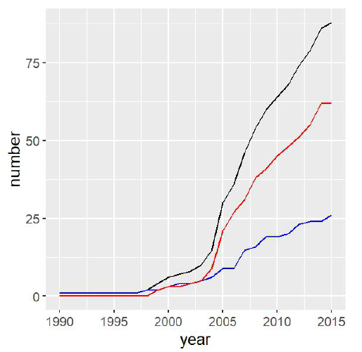
We have used the information on existing vineyards in the Małopolska region, which are available for download at http://www.winogrodnicy.pl. The data have been manually collected over some time, though each vineyard owner is also free to register his/her vineyard at the web page. These data contain, among other things, information on the vineyard's owner, location, area and the year in which it was established. We accessed the data in June 2016, and so the last year under consideration was 2015, with 88 existing vineyards (Figure 1). We have also used regional data on community area, number of inhabitants, number of farms (divided into large farms over 1 ha. and small farms below 1 ha.) as well as the number of tourist attractions in a particular community. The data come from common agricultural census (2002 and 2010). The data were interpolated and extrapolated (by assigning the time period limit values) to cover the period 1990 until 2015. As the data are relatively stable over time, such a procedure had minimal impact on the results. The source of the data is the Polish Statistical Office. Furthermore, geographical data on average altitude above sea level for each community and information as to whether a community lies on the border of the Małopolska region, were all utilised.
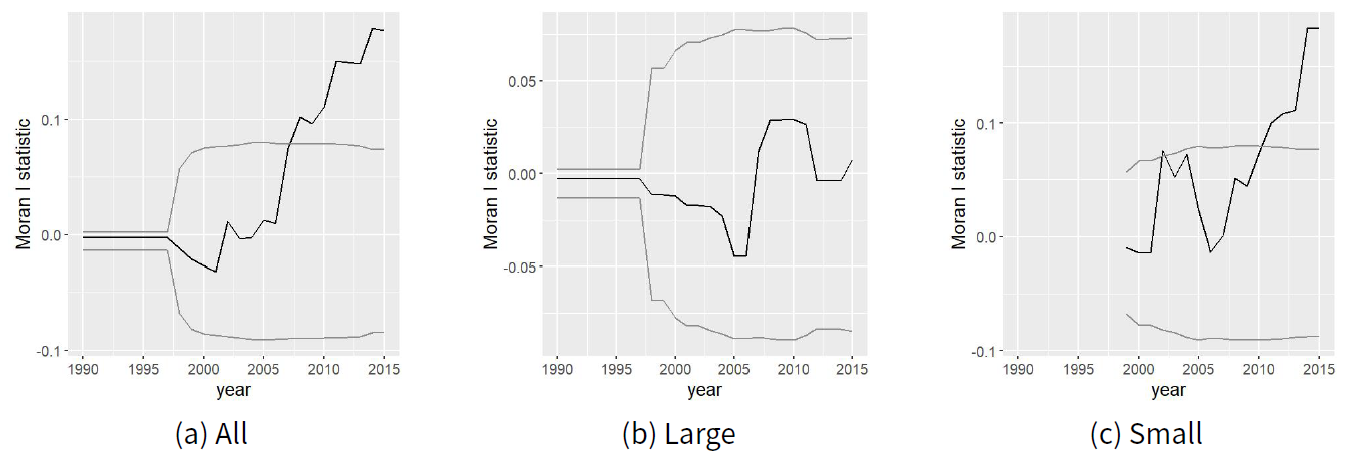
We have analysed development of the total (large and small) number of vineyards in the period 1990-2015, in addition to their geographical concentration. This latter feature was measured by Moran's \(I\) test, whose formula is given by Equation 1, we conventionally assumed that \(w_{ii} =0\).
| $$I=\frac n{\sum_{ij}w_{ij}}\frac{\sum_{ij}w_{ij}(x_i-\overline{x})(x_j- \overline{x})}{\sum_i(x_i-\overline{x})^2}$$ | (1) |
The Moran \(I\) statistic was originally developed by Moran (1948). Let us consider \(n\) different regions arranged in 2-dimensional space. Let us also define the neighbourhood structure represented by \(n\times n\) matrix whose \(i,j\) element accepts the value 1 if both regions: \(i\) and \(j\) are spatial neighbours. In our paper, we denote two different communities as neighbours if they have a common border. The symbol \(x_i\) represents the value of a variable \(x\) under consideration in a region \(i\). In particular, \(x_i\) represents the number of vineyards in \(i\) community. Moran \(I\) measures the spatial correlation of variable \(x_i\), giving an indication of whether the regions with relatively high (low) values of variable \(x\) are clustered or are randomly distributed in a space. In general, the Moran \(I\) statistic is bounded by \(-1\) and \(1\). The value \(-1\) indicates perfect dispersion and the value \(1\) indicates perfect clustering (all vineyards in the same community).
The detailed map with arrangement of the vineyards as of January 2018 is presented in Figure 2.

Figure 3 shows the calculated real Moran \(I\), together with a 95% confidence interval around the expected value (assuming no spatial concentration), for: total, large, and small vineyards for the period 1990-2015. The (c) panel of the Figure 3 shows the increasing spatial concentration of the small vineyards over time, whereas large vineyards – panel (b) – remain evenly distributed in the Małopolska district. The jump observed in confidence interval lines for large vineyards in 1998 results from the fact that until 1997 only one large vineyard existed and the second one was established in 1998. Similarly, the first two small vineyards were established in 1999.
Econometric model
Let us consider the following dynamic model of vineyard development:
| $$y_t = \rho W y_{t-1} + X\beta + \epsilon_t$$ | (2) |
By subsequent substitution of \(y_{t-i}\) in the Formula 2, followed by grouping of the relevant variables, introducing variable \(\epsilon\) and finally dropping the time subscripts, we obtain the spatial lag model, or a mixed regressive, spatial autoregressive model equation, in the form presented in Anselin (2001):
| $$y = \rho W y + X\beta + \epsilon $$ | (3) |
Regression results are presented in Table 3, where \(\rho\) = 0.016741 with p-value: 0.44871. Parameter \(\rho\) provides information on the strength of spatial auto-regression relations, the influence of the vineyards number on the vineyards numbers in the neighbouring communities. We considered the following independent variables \(X\) in the regression analysis: area, number of farms, number of inhabitants, number of tourist attractions in a given community. Moreover, we consider two binary variables: heigth_bin, which takes the value 1 if the average altitude above sea level exceeds 500 in a particular community (insufficient climate conditions for vine growing) and 0 otherwise, and border_community, which takes the value 1 if a given community lies at the border of Malopolska district and 0 otherwise. As the latter is insignificant, we did not take this effect into account (missing neighbouring communities that are not in the Malopolska district) in our model. We can observe that the number of farms significantly positively influences the number of vineyards observed in the particular community. The height_bin has significantly negative effect on the number of vineyards observed. The vineyards observed in the neighbouring communities seemed to slightly positively influence the number of vineyards in the particular community (the effect is however, insignificant).
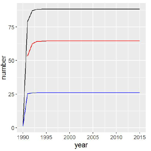
Based on the estimated parameters, we iteratively calculated the number of vineyards in each community according to equation to Equation 2. The estimated results are shown in Figure 4. A solid line indicates the total estimated number of vineyards, a blue line the number of large vineyards and a red line number of small vineyards.
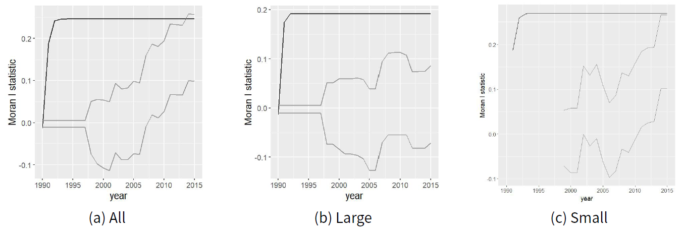
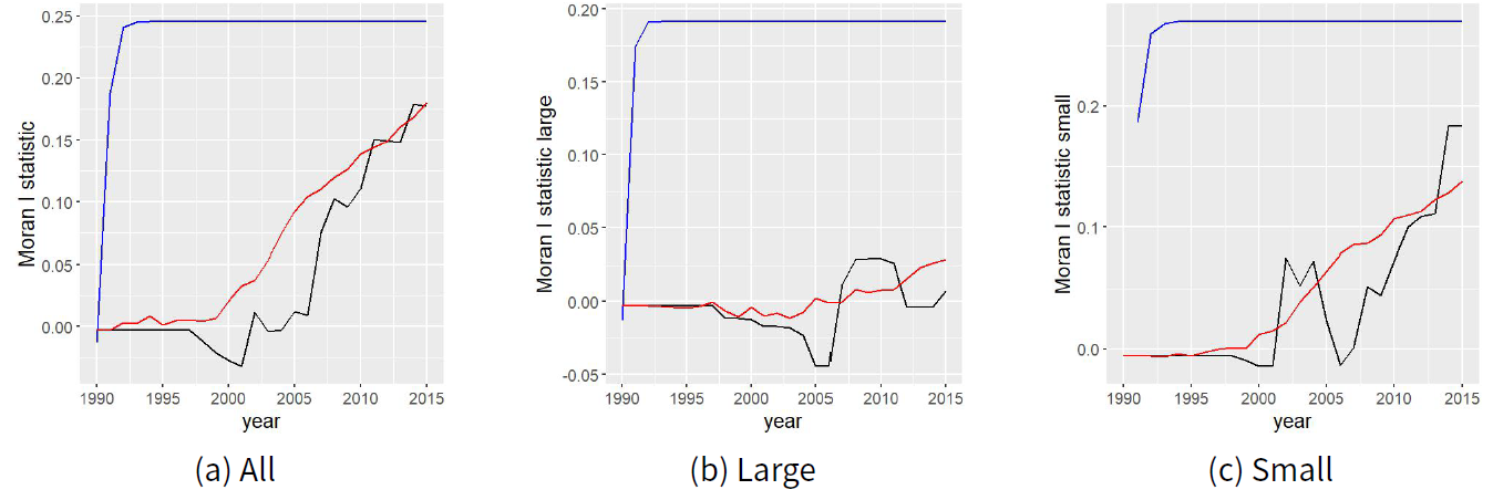
In addition, the Moran I statistic values have been calculated and are shown in Figure 5. Black lines show Moran I statistic values for theoretical values (estimated using the spatial auto-regression model) of vineyards, whereas grey lines show lower and upper 95% confidence intervals around truly observed values. In general, we can observe that SAR regression correctly (estimated values lie within 95% confidence intervals) estimates the current (2015) quantity and spatial dependence (with the exception of spatial dependence for large vineyards), even though it fails to adequately capture the dynamics of the process (it underestimates \(\rho\) parameter values).
| Variable | Estimate | Std. Error |
| (Intercept) | 0.30100 | 0.21200 |
| area | -0.00004 | 0.00004 |
| farms | 0.00020** | 0.00010 |
| people | -0.00000 | 0.00001 |
| tourism | -0.00040 | 0.00300 |
| border_community | -0.08400 | 0.08800 |
| heigth_bin | -0.50300** | 0.19800 |
| Observations | 182 | |
| Log Likelihood | -274.904 | |
| \(\sigma^{2}\) | 1.159 | |
| Akaike Inf. Crit. | 567.808 | |
| Wald Test | 0.716 (df = 1) | |
| LR Test | 0.574 (df = 1) |
We also conducted the regression analysis separately for large and small vineyards. In addition, a more advanced model – the simple panel space auto-regression model – was applied. This model takes into account the entire data history and is a natural extension of the model (3). Namely, we have estimated the parameters of the following panel model (4), see. Millo et al. (2012):
| $$y = \rho \left(I_T \otimes W \right) y + X\beta + \epsilon $$ | (4) |
The time dynamics are not considered in explicit ways in either of the models (3) and (4). Therefore, we also estimated the STAR (space time autoregressive model) where spatial and time dependence is considered simultaneously. These models have the general form:
| $$z_t = \sum_{k=1}^{p} \sum_{l=0}^{\lambda_k} \phi_{kl}W^{(l)} z_{t-k} + \epsilon $$ | (5) |
Agent-Based Modelling of Vineyard Development
In this section, we present the design of the proposed agent-based model, the results of its calibration and its sensitivity analysis.
Agent-based model
We considered the following agents in our model: (i) small and large farms, (ii) small and large vineyards. We also considered 182 communities of the Małopolska region. Each community is characterised by the climate factor \(c_c\). Additionally, there is a critical climate factor \(c_c^{critical}\) such that the vineyards can be established in a particular community only if \( c_c \ge c_c^{critical}\). As the altitude above sea level is the main factor that distinguishes weather conditions in different communities of the Malopolska region, we empirically assumed that the growing of wine grapes is only possible for those communities with an average altitude less than 500m above sea level. We first modelled the enthusiasm dynamics, whereby we treated enthusiasts as farm owners interested in wine but not necessarily in wine production itself. The probability that a wine-making enthusiast appears on a farm is defined by the equation:
| $$P_E = b_E + \lambda_{E\rightarrow E}f(N_E^S+N_E^L)+ \lambda_{V^S\rightarrow E}f(N_V^S) +\lambda_{V^L\rightarrow E}f(N_V^L)$$ | (6) |
| $$P_V^S = b_V^S + b_{2004\rightarrow V}^S + \lambda_{E\rightarrow V}^Sf(N_E^S+N_E^L)+ \lambda_{V^S\rightarrow V}^Sf(N_V^S) +\lambda_{V^L\rightarrow V}^Sf(N_V^L)$$ | (7) |
| $$P_V^L = b_V^L + b_{2004\rightarrow V}^L + \lambda_{E\rightarrow V}^Lf(N_E^S+N_E^L) + \lambda_{V^S\rightarrow V}^Lf(N_V^S) + \lambda_{V^L\rightarrow V}^Lf(N_V^L)$$ | (8) |
The owner of the large farm may decide for various reasons (e.g., his/her own free choice or if only a subsection of the farm area is suitable for vine growing) to establish only a small vineyard. As we only possessed data on the total area of the farm, we used a simplified approach. Namely, we assigned large farms to small ones (with a probability described by a parameter \(p_{L\rightarrow V^S}\)) to model the transformation of the large farm to a small vineyard. In each round, an existing vineyard can also be shut down with the probability \(P_V^{EXP}\).
The model is implemented in Java, using the MASON 19 framework. The code is available at the following address: https://www.comses.net/codebases/5891/releases/1.1.0/. We consider three main classes of agents, namely: communities, large and small farms. Each farm can only belong to one given community. Each farm can be in one of the following states at each step: regular farm, wine enthusiast and vineyard. The flows between different agent states is shown in Figure 7.
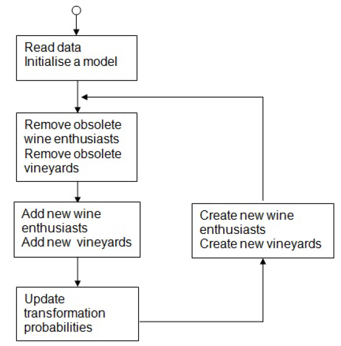
At each step, firstly we randomly decided whether a vineyard has ceased to exist (transforms to a regular farm) or a wine enthusiast has lost interest in wine (also transforms to a regular farm). Then, additionally created vineyards and enthusiasts from the previous step are added to the existing pools of vineyards and wine enthusiasts in each community separately. Having updated the transformation probabilities for each community, we randomly decided whether a regular farm could transform into a wine enthusiast (firstly, under the provision that community climate conditions permit this. Secondly under the provision that the required minimum number of wine enthusiasts in a community or pre-existing vineyard is satisfied), and whether a wine enthusiast can transform into a vineyard in the current step. The new vineyards and wine enthusiasts are added to the existing pools at the beginning of the subsequent step. The general flow of the simulation in presented in Figure 8.
Results
For each of the 10 000 parameter sets, we simulated the development of potential vineyards 64 times. Each single parameter set was selected, using Sobol numbers sequence (Christophe & Petr 2015), from the entire parameter space, which is defined as the Cartesian product of permissible parameter values for each of the parameters, as defined in Table 4. The parameter space was constructed using the results of the econometric analysis. Generally, we used the order of magnitude of the estimated parameter \(\rho\) and inferred the signs of parameters \(\lambda_{V^L\rightarrow V}^L\) and \(\lambda_{V^S\rightarrow V}^L\).
This led to 640 000 development paths covering the period 1990 to 2015. Each step represents a year. Firstly, we determined the parameter sets that enable the reconstruction of the real development path of vineyards in the Małopolska region. We selected parameter sets so that the simulated large and small vineyards numbers and respective Moran \(I\) statistics are close to the real observed values. Bert et al. (2014) distinguished between conceptual and empirical validation. The first was based on iterative communication with stake holders and domain experts and the second on an iterative model calibration process. We used literature overview and a survey results for conceptual validation and applied the method of simulated moments (MSM), see Gourieroux & Monfort (1996) and Kamiński & Koloch (2017) for empirical validation. In particular, and using the original notation of Gourieroux & Monfort (1996), we are looking for such a parameter vector \(\theta\) that minimises:
| $${\left[\sum_{t=1}^{T} Z_t\left(K(y_t,z_t) -\frac{1}{S} \sum_{i=1}^{S} \overline{k}(z_t,u_i^s,\theta)\right)\right]}^t \Omega {\left[\sum_{t=1}^{T} Z_t\left(K(y_t,z_t) -\frac{1}{S} \sum_{i=1}^{S} \overline{k}(z_t,u_i^s,\theta)\right)\right]} $$ | (9) |
| symbol | variable | lower value | upper value |
| a | \(P_V^{EXP}\) | 0 | 0.05 |
| b | \(P_E^{EXP}\) | 0 | 0.2 |
| c | \(b^L_V\) | 0 | 0.001 |
| d | \(\lambda_{E\rightarrow V}^L\) | 0 | 0.001 |
| e | \(\lambda_{V^L\rightarrow V}^L\) | -0.001 | 0 |
| f | \(\lambda_{V^S\rightarrow V}^L\) | 0 | 0.001 |
| g | \(b^S_V\) | 0 | 0.001 |
| h | \(\lambda_{E\rightarrow V}^S\) | 0 | 0.001 |
| i | \(\lambda_{V^L\rightarrow V}^S\) | 0 | 0.001 |
| j | \(\lambda_{V^S\rightarrow V}^S\) | 0 | 0.001 |
| k | \(N_E^{critical}\) | 0 | 10 |
| l | \(\lambda_{V^L\rightarrow E}\) | 0 | 0.001 |
| m | \(\lambda_{V^S\rightarrow E}\) | 0 | 0.001 |
| n | \(\lambda_{E\rightarrow E}\) | 0 | 0.001 |
| o | \(b_E\) | 0 | 0.001 |
| p | \(p_{L\rightarrow V^S}\) | 0.2 | 0.8 |
| q | \(b_{2004\rightarrow V}^S\) | 0 | 0.004 |
| r | \(b_{2004\rightarrow V}^L\) | 0 | 0.004 |
| parameter | value |
| \(P_V^{EXP}\) | 0.03734 |
| \(P_E^{EXP}\) | 0.159542 |
| \(b^L_V\) | 0.00069 |
| \(\lambda_{E\rightarrow V}^L\) | 0.00026 |
| \(\lambda_{V^L\rightarrow V}^L\) | -0.00091 |
| \(\lambda_{V^S\rightarrow V}^L\) | 0.00058 |
| \(b^S_V\) | 0.00038 |
| \(\lambda_{E\rightarrow V}^S\) | 0.00004 |
| \(\lambda_{V^L\rightarrow V}^S\) | 0.00078 |
| \(\lambda_{V^S\rightarrow V}^S\) | 0.00015 |
| \(N_E^{critical}\) | 2 |
| \(\lambda_{V^L\rightarrow E}\) | 0.00073 |
| \(\lambda_{V^S\rightarrow E}\) | 0.00056 |
| \(\lambda_{E\rightarrow E}\) | 0.00068 |
| \(b_E\) | 0.00046 |
| \(p_{L\rightarrow V^S}\) | 0.72112 |
| \(b_{2004\rightarrow V}^S\) | 0.00382 |
| \(b_{2004\rightarrow V}^L\) | 0.00265 |
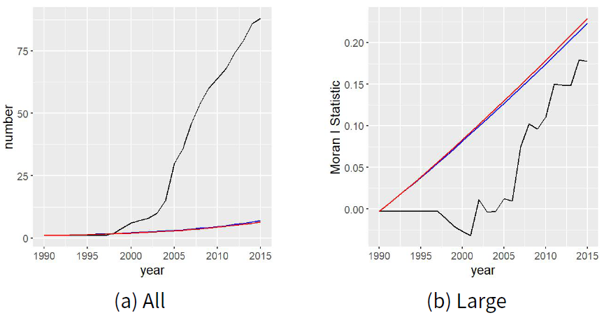
To sum up, we present a comparison of the true observed dynamics of vineyard development with both econometric modelling results and simulation results for the selected parameter set (average path over 64 replications of simulation). The dynamics of vineyard quantity is shown in Figure 9. The black line shows real observed values, the blue line shows the regressions results and the red line shows the simulation result. Similarly, the dynamics of vineyard concentration (measured by Moran \(I\) statistics) is presented in Figure 10. We can observe significantly closer fit in case of simulation results.

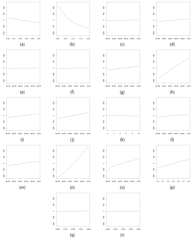
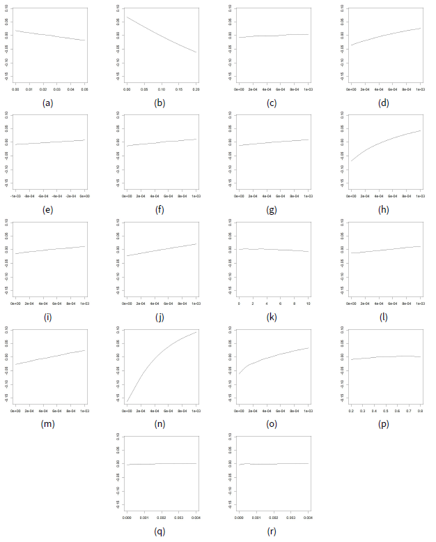
Secondly, we analysed which parameters played a significant role in the development of the vineyards in the Małopolska district. For this purpose, two generalised additive metamodels were estimated (Wood 2017). The purpose of the procedure was to evaluate how sensitive are the simulation results (number of vineyards and concentration as measured by Moran \(I\) statistic value in 2015) with respect to different parameter values. Application of generalized additive models admits the linear additive representation, thus we can evaluate what is the influence of each of the parameters considered on the result separately. Moreover, the applied procedure allows for nonlinear influence. In the first model, the independent variable is the total number of vineyards in 2015, while the second model uses the Moran \(I\) statistic value in 2015 for all vineyards (independent of farm size) instead, see Equation 10:
| $$y_i=\alpha_0 +\sum_{i=1}^{N_p} s(\theta_i) + \epsilon_i, $$ | (10) |
Equation 6 describes the diffusion of enthusiasm and Equations 7 and 8 formation of a vineyard. We can observe that the estimated values of the parameters used in these equations are of similar magnitude, see Table 5. This suggests that both social and individual aspects played a similar role in the dynamics of the vineyard formation process. We can also observe that an existing large vineyard attracts new small vineyards as well as existing small vineyards attracting new large vineyards. This can potentially be explained by micro-climates that are advantageous for viticulture, alongside potential benefits from cooperation. The critical number of enthusiasts necessary to establish an initial vineyard in a particular community is relatively low (equal to 2) suggesting that vineyard creation is of an individual character once someone is an enthusiast. The values related to additional external influences in 2004 are around 10 times larger than observed values of parameters. This suggest a substantial impact from intensive training and promotional campaigns as well as additional funds for the farmers (in 2004 Poland joined EU).
There is a group of the most significant parameters, when interpreting the results of the sensitivity analysis carried out using generalized additive models. These parameters \(P_E^{EXP}\), \(\lambda_{E\rightarrow V}^S\), \(\lambda_{V^L\rightarrow V}^S\), \(\lambda_{V^S\rightarrow E}\), \(\lambda_{E\rightarrow E}\), \(b_E\), and \(p_{L\rightarrow V^S}\) only for number but not for concentration fall into three groups. The first group of parameters: \(b_E\), \(\lambda_{E\rightarrow E}\),and \(P_E^{EXP}\) govern the wine enthusiast number by specifying the probability of spontaneous appearance of enthusiasm, social influence of wine enthusiasts (attracting next new wine enthusiasts), and the tendency to extinguish enthusiasm. The second group of parameters: \(\lambda_{E\rightarrow V}^S\) and \(\lambda_{V^L\rightarrow V}^S\) govern the transformation process of wine enthusiasts to small vineyards and the influence of the existing large vineyard on the new small vineyards. Additionally parameter \(p_{L\rightarrow V^S}\) defines what percentage of large farms can only transform to small vineyards (only part of the farm is used for growing vines).
Concluding Remarks and Further Research
The processes of viticulture and wine production in the Małopolska region have been actively developing for the last 30 years. In addition to structural changes in the market (e.g., advances in vine cultivation, shifts in consumer preferences toward wine), behavioural and social factors have also played a significant role in this process.
In this paper, we have proposed an agent-based model that includes a behavioural component (wine enthusiasm), in order to simulate subsequent development of the local wine sector. The drawback of having a relatively short history for the relevant data is countered by its relevance to a current situation. This has enabled us to collect high quality empirical data for the entire period, which were used to validate the proposed agent-based model quantitatively and qualitatively. In particular, the analysis of the available evidence revealed strong clustering effects namely, a relatively large number of vineyards originate at a relatively similar time and place.
The proposed agent-based model puts more emphasis on spatial relations and less on the decision process. We implemented heterogeneous agents (small and large farms) and defined three potential states for the agents; regular farm, wine enthusiast and vineyard, and then we modelled the transition process. These probabilities depend on the set of parameters and spatial relations. We estimated the model parameters using the Method of Simulated Moments. Our key findings are as follows:
- The agent-based model has a significantly superior predictive power compared to standard econometric models.
- The values of the estimated parameters of the agent-based model support the hypotheses we have formulated, in particular; there is no single predominant factor that influences wine region development (an array of social, economic and micro-climate factors matter) and behavioural factors of a social character play a significant role. The estimated parameters in equations in Equations: 6, 7, and 8 are of similar magnitude, whereas 6 represents social (behavioural) phenomena, and 7, and 8 represent individual (economic) phenomena.
- The sensitivity analysis of the agent-based model allowed us to understand what key factors have driven viticulture development in the Małopolska region. In particular, the spontaneous appearance and social diffusion of wine enthusiasm and the process of establishing small vineyards by enthusiasts, influenced by the presence of a large vineyard in the same or neighbouring community.
- The model allowed us to capture the emergent two-step vineyard development mechanism, involving community building and vineyard creation phases. This mechanism has proven crucial to ensuring its observed predictive power.
The model and analysis can potentially be extended in two ways. Firstly, one could give a more explicit consideration to institutional restrictions (wine production is subject to numerous regulations, according to greater complexity and volume of output) and the role of winemaker associations. Secondly, the model could be applied to analyse the dynamics of other wine regions.
Acknowledgements
We would like to thank the wine producers of Małopolska region for the discussions and participation in the survey. We also benefited from the dicussions with the participants of AAWE (American Association of Wine Economists) Conference in Bordeaux 2016 at the early stage of our research. We also thank two anonymous reviewers for their comments. This research was supported by a grant awarded by the National Science Centre of Poland under the project title “Behavioural and microstructural aspects of the financial and alternative investments markets,” Decision no. 2015/17/B/HS4/02708.Appendix: Generalized additive model results
The estimated splines for generalized additive models (GAM) are presented in this Appendix. The meaning of the labels used (consecutive letters of the alphabet) for the individual graphs are explained in Table 4. Figure 11 shows the spline for a GAM model with the total number of vineyards as the dependent variable, whereas Figure 12 shows the same but with the Moran I value as the dependent variable.
References
ANSELIN, L. (2001). Spatial econometrics. In Baltagi, B. H. (Ed), A companion to theoretical econometrics. Chichester: Wiley-Blackwell, pp. 310-330.
ARNDT, J. (1967). Role of product-related conversations in the diffusion of a new product. Journal of marketing Research, 4(3), 291-295.
ASHENFELTER, O. & Storchmann, K. (2010). Measuring the economic effect of global warming on viticulture using auction, retail, and wholesale prices. Review of Industrial Organization, 37(1), 51-64. [doi:10.1007/s11151-010-9256-6]
ASHENFELTER, O. & Storchmann, K. (2010). Using hedonic models of solar radiation and weather to assess the economic effect of climate change: The case of Mosel valley vineyards. Review of Economics and Statistics, 92(2), 333–349.
ASHENFELTER, O. & Storchmann, K. (2016). The economics of wine, weather, and climate change. Review of Environmental Economics and Policy, 10(1), 25–46. [doi:10.1093/reep/rev018]
BARDAJI, I. & Iraizoz, B. (2015). Uneven responses to climate and market influencing the geography of high-quality wine production in Europe. Regional environmental change, 15(1), 79–92.
BASS, F. M. (1969). A new product growth for model consumer durables. Management science, 15(5), 215–227. [doi:10.1287/mnsc.15.5.215]
BELICH, J. (2009). Replenishing the earth: The settler revolution and the rise of the Angloworld. Oxford: Oxford University Press.
BENTZEN, J., & Smith, V. (2009). Wine production in Denmark Do the characteristics of the vineyards affect the chances for awards? Working Papers, University of Aarhus (No. 09-21).
BERGER, T. (2001). Agent-based spatial models applied to agriculture: a simulation tool for technology diffusion, resource use changes and policy analysis. Agricultural economics, 25(2-3), 245–260.
BERGER, T., Schreinemachers, P. & Woelcke, J. (2006). Multi-agent simulation for the targeting of development policies in less-favored areas. Agricultural Systems, 88(1), 28–43. [doi:10.1016/j.agsy.2005.06.002]
BERT, F. E., Rovere, S. L., Macal, C. M., North, M. J. & Podestá, G. P. (2014). Lessons from a comprehensive validation of an agent based-model: The experience of the Pampas model of Argentinean agricultural systems. Ecological modelling, 273, 284–298.
BOUZDINE-CHAMEEVA, T. & Galam, S. (2011). Word-of-mouth versus experts and reputation in the individual dynamics of wine purchasing. Advances in Complex Systems, 14(6), 871–885. [doi:10.1142/S0219525911003475]
BRADY, M., Sahrbacher, C., Kellermann, K. & Happe, K. (2012). An agent-based approach to modeling impacts of agricultural policy on land use, biodiversity and ecosystem services. Landscape Ecology, 27(9), 1363–1381.
CASSI, L., Morrison, A. & Ter Wal, A. L. (2012). The evolution of trade and scientific collaboration networks in the global wine sector: A longitudinal study using network analysis. Economic geography, 88(3), 311–334. [doi:10.1111/j.1944-8287.2012.01154.x]
CHEVET, J.-M., Lecocq, S. & Visser, M. (2011). Climate, grapevine phenology, wine production, and prices: Pauillac (1800–2009). The American Economic Review, 101(3), 142–146.
CHEYSSON, F. (2016). Modelling Space Time AutoRegressive Moving Average (STARMA) Processes. R package version 1.3: https://cran.r-project.org/web/packages/starma/index.html.
CHRISTOPHE, D. & Petr, S. (2015). Randtoolbox: Generating and Testing Random Numbers. R package version 1.17.
CONWAY, J. (1970). The game of life. Scientific American, 223(4), 4.
CORBY, J. H. K. (2010). For members and markets: Neoliberalism and cooperativism in Mendoza’s wine industry. Journal of Latin American Geography, 9(2), 27–47.
CZUPRYNA, M., & OLEKSY, P. (2014). Development potential of commodity exchanges in CEE region: Case study of the Polish wine market. In M. Ninnaj & M. Záhumenská (Eds.), Proceedings of the 16th International Scientific Conference Finance and Risk 2014, 1. Bratislava: Ekonóm, pp. 54-63.
DALMORO, M. (2013). The formation of country wineries networks for internationalization: An analysis of two new world wines regions. Journal of wine research, 24(2), 96–111.
DE Salvo, M., Capitello, R. & Begalli, D. (2014). The estimation of climate change impacts on the adoption of sustainable production processes in viticulture: A multidisciplinary approach. Competitiveness of Agro-Food and Environmental Economy, 10.
DELAY, E., Chevallier, M., Rouvellac, É., & Zottele, F. (2015). Effects of the Wine Cooperative System on Socio-economic Factors and Landscapes in Mountain Areas. Journal of Alpine Research| Revue de Géographie Alpine, 103-1.
DOLOREUX, D. & Lord-Tarte, E. (2012). Context and differentiation: Development of the wine industry in three Canadian regions. The Social Science Journal, 49(4), 519–527. [doi:10.1016/j.soscij.2012.04.002]
FARMER, J. D. & Foley, D. (2009). The economy needs agent-based modelling. Nature, 460(7256), 685–686.
FILATOVA, T., Verburg, P. H., Parker, D. C. & Stannard, C. A. (2013). Spatial agent-based models for socio-ecological systems: Challenges and prospects. Environmental modelling & software, 45(81), 1–7. [doi:10.1016/j.envsoft.2013.03.017]
GADE, D. W. (2004). Tradition, territory, and terroir in French viniculture: Cassis, France, and appellation contrôlée. Annals of the Association of American Geographers, 94(4), 848–867.
GARCIA, R. & Atkin, T. (2007). Coopetition for the diffusion of resistant innovations: A case study in the global wine industry using an agent-based model. In 25th International Conference of the System Dynamics Society, Boston, MA.
GERGAUD, O. & Ginsburgh, V. (2008). Natural endowments, production technologies and the quality of wines in Bordeaux. Does terroir matter? The Economic Journal, 118(529).
GIULIANI, E. (2013). Clusters, networks and firms’ product success: an empirical study. Management Decision, 51(6), 1135–1160. [doi:10.1108/MD-01-2012-0010]
GIULIANI, E. & Bell, M. (2005). The micro-determinants of meso-level learning and innovation: evidence from a Chilean wine cluster. Research policy, 34(1), 47–68.
GOLDENBERG, J., Libai, B., Moldovan, S. & Muller, E. (2007). The NPV of bad news. International Journal of Research in Marketing, 24(3), 186–200. [doi:10.1016/j.ijresmar.2007.02.003]
GOURIEROUX, M., Gourieroux, C., Monfort, A., & Monfort, D. A. (1996). Simulation-Based Econometric Methods. Oxford: Oxford University Press.
GROENEVELD, J., Müller, B., Buchmann, C. M., Dressler, G., Guo, C., Hase, N., Hoffmann, F., John, F., Klassert, C., Lauf, T. et al. (2017). Theoretical foundations of human decision-making in agent-based land use models - A review. Environmental modelling & software, 87(1), 39–48. [doi:10.1016/j.envsoft.2016.10.008]
HAPPE, K., Kellermann, K. & Balmann, A. (2006). Agent-based analysis of agricultural policies: an illustration of the agricultural policy simulator Agripolis, its adaptation and behavior. Ecology and Society, 11(1).
JANSSEN, M. A. & Ostrom, E. (2006). Empirically based, agent-based models. Ecology and society, 11(2). [doi:10.5751/ES-01861-110237]
KAMIŃSKI, B. & Koloch, G. (2017). Output analysis for terminating simulations with partial observability. Simulation Modelling Practice and Theory, 71, 102–113.
KIESLING, E., Günther, M., Stummer, C. & Wakolbinger, L. M. (2012). Agent-based simulation of innovation diffusion: A review. Central European Journal of Operations Research, 20(2), 183–230. [doi:10.1007/s10100-011-0210-y]
KOLASA, A. (2017). Life cycle income and consumption patterns in Poland. Central European Journal of Economic Modelling and Econometrics, 9, 137–172.
KOWALSKA-STYCZEŃ, A. & Sznajd-Weron, K. (2016). From consumer decision to market share–unanimity of majority? Journal of Artificial Societies and Social Simulation, 19(4), 10: https://www.jasss.org/19/4/10.html. [doi:10.18564/jasss.3156]
KREBS, F. (2017). An empirically grounded model of green electricity adoption in Germany: Calibration, validation and insights into patterns of diffusion. Journal of Artificial Societies and Social Simulation, 20(2), 10: https://www.jasss.org/20/2/10.html. [doi:10.18564/jasss.3429]
LI, H., de Zubielqui, G. C., & O’Connor, A. (2015). Entrepreneurial networking capacity of cluster firms: a social network perspective on how shared resources enhance firm performance. Small Business Economics, 45(3), 523-541. [doi:10.1007/s11187-015-9659-8]
LOBIANCO, A. & Esposti, R. (2010). The regional multi-agent simulator (regmas): An open-source spatially explicit model to assess the impact of agricultural policies. Computers and Electronics in Agriculture, 72(1), 14–26.
MACAL, C. M. & North, M. J. (2010). Tutorial on agent-based modelling and simulation. Journal of Simulation, 4(3), 151–162. [doi:10.1057/jos.2010.3]
MAHAJAN, V., Muller, E., & Bass, F. M. (1991). New product diffusion models in marketing: A review and directions for research. In N. Nakicenovic & A. Grübler (Eds.), Diffusion of technologies and social behavior. Berlin, Heidelberg: Springer, pp. 125-177.
MATTHEWS, R. B., Gilbert, N. G., Roach, A., Polhill, J. G. & Gotts, N. M. (2007). Agent-based land-use models: A review of applications. Landscape Ecology, 22(10), 1447–1459. [doi:10.1007/s10980-007-9135-1]
MCINTYRE, J., Mitchell, R., Boyle, B. & Ryan, S. (2013). We used to get and give a lot of help: Networking, co-operation and knowledge flow in the hunter valley wine cluster. Australian Economic History Review, 53(3), 247–267.
MILLO, G., Piras, G.(2012) SPLM: Spatial panel data models in R. Journal of Statistical Software, 47(1), 1-38. [doi:10.18637/jss.v047.i01]
MORAN, P. A. (1948). The interpretation of statistical maps. Journal of the Royal Statistical Society. Series B (Methodological), 10(2), 243–251.
OVERTON, J. & Banks, G. (2015). Conspicuous production: Wine, capital and status. Capital & Class, 39(3), 473–491. [doi:10.1177/0309816815607022]
ROSS, R. B. & Westgren, R. E. (2009). An agent-based model of entrepreneurial behavior in agri-food markets. Canadian Journal of Agricultural Economics/Revue canadienne d’agroeconomie, 57(4), 459–480.
RYTKÖNEN, P. (2013). Sweden - An emerging wine country - A case of innovation in the context of the" new rurality". Spanish Journal of Rural Development, 4(4). [doi:10.5261/2013.GEN4.08]
SCHELLING, T. C. (1971). Dynamic models of segregation. Journal of Mathematical Sociology, 1(2), 143–186.
SCHMITT, F. (2015). Die wettbewerbssituation von winzergenossenscha en: am beispiel der bergsträsser winzer eg. Zeitschri für das gesamte Genossenscha swesen, 65(2), 121–134.
SCHREINEMACHERS, P. & Berger, T. (2011). An agent-based simulation model of human–environment interactions in agricultural systems. Environmental Modelling & Software, 26(7), 845–859.
SCHULTZ, H. R. (2016). Global climate change, sustainability, and some challenges for grape and wine production. Journal of Wine Economics, 11(1), 181–200. [doi:10.1017/jwe.2015.31]
SCHWARZ, N. & Ernst, A. (2009). Agent-based modeling of the diffusion of environmental innovations - An empirical approach. Technological Forecasting and Social Change, 76(4), 497–511.
SCOTT Morton, F. M. & Podolny, J. M. (2002). Love or money? The effects of owner motivation in the California wine industry. The Journal of Industrial Economics, 50(4), 431–456. [doi:10.1111/1467-6451.00185]
SHAW, T. B. (2017). Climate change and the evolution of the Ontario cool climate wine regions in Canada. Journal of Wine Research, 28(1), 13–45.
STACHANCZYK, A. & Tutaj, J. (2016). Agriculture in Lesser Poland Voivodship in 2015. The Statistical Office in Cracow.
SWAMINATHAN, A. (2001). Resource partitioning and the evolution of specialist organizations: The role of location and identity in the US wine industry. Academy of Management Journal, 44(6), 1169–1185.
SWAMINATHAN, A. & Delacroix, J. (1991). Differentiation within an organizational population: Additional evidence from the wine industry. Academy of Management Journal, 34(3), 679–692.
THIRIOT, S. & Kant, J.-D. (2008). Using associative networks to represent adopters’ beliefs in a multiagent model of innovation diffusion. Advances in Complex Systems, 11(02), 261–272.
TISSOT, C., Rouan, M., Neethling, E., Quenol, H., & Brosset, D. (2014). Modeling of vine agronomic practices in the context of climate change. In BIO Web of Conferences (Vol. 3, p. 01015). EDP Sciences. [doi:10.1051/bioconf/20140301015]
TÓTH, J. & Végvári, Z. (2016). Future of winegrape growing regions in Europe. Australian Journal of Grape and Wine Research, 22(1), 64–72.
VAN Leeuwen, C. & Darriet, P. (2016). The impact of climate change on viticulture and wine quality. Journal of Wine Economics, 11(1), 150–167. [doi:10.1017/jwe.2015.21]
WOOD, S. N. (2017). Generalized additive models: an introduction with R. CRC Press.