
Introduction
Agent-based models (ABMs) use a bottom-up approach to discover complex, aggregate-level properties. These properties emerge from individual agent behaviors and interactions within their environment. Thus, once individual behavioral rules of Bitcoin trading are formulated, an ABM can generate an emerging aggregate phenomenon, such as market price, from the possibly non-linear interactions of those rules. Unfortunately, discovering these rules can be challenging and potentially require deep insight and domain knowledge.
We utilize inverse reinforcement learning (IRL) as a method for obtaining individual rules for an ABM directly from data. Conventional statistical analysis of trading behaviors or market behaviors mainly evaluates the impact of independent actions on the target events. However, we exploit Markov decision processes (MDPs) to model the long-term process of trading Bitcoin, and then estimate a generalizable trading rule for each agent assuming an action has a long-term consequence, and each agent tries to maximize their long-term rewards.
With the combination of IRL & ABM, initially proposed by Lee et al. (2017), we first generate synthetic but realistic Bitcoin trading rules and, then, find daily prices resulting from the interactions. Through an experiment, we show that the method provides rich but concise market behavioral rules for agents while predicting aggregate-level market price. The contribution of this paper is to demonstrate that the combination of individually learned rules and macro-level simulations can provide a new option for market prediction and policy experiments.
In Section 2 we review the background of cryptocurrency, IRL, and related research. In Section 3, we present the details of the proposed method. Section 4 presents an experiment and results using the proposed method on nine 3-month periods of the Bitcoin market. In Section 5 we discuss the challenges of the method, and we conclude the paper by highlighting areas of future research in Section 6.
Background and Related Work
Cryptocurrency and blockchain
Blockchain first came into existence in 2009 as a result of the seminal paper, "Bitcoin: A Peer-to-Peer Electronic Cash System" published under the pseudonym "Satoshi Nakamoto" (Nakamoto 2008). The proposition of the paper was simple: to create a distributed public ledger upon which everybody could participate and interact to maintain a record of transactions, removing the necessity of any third party intermediary. Essentially, the paper proposed a way of transacting currency without the need for a bank or central body to govern or dictate the flow of assets in a secure and distributed way.
The Bitcoin blockchain is secured thanks to cryptography, and as a result, it is nearly impossible to steal or take an individual’s Bitcoins. Bitcoin is able to secure itself using a network of what are called "miners" who search for what are called "blocks" of Bitcoin using a large array of computers competitively validating the integrity of transactions and in turn getting rewarded with newly minted Bitcoin. All of Bitcoin’s transaction history is available on the public blockchain, including every transaction ever made since its genesis block and will continue to exist as long as the network remains operational and at least one copy of it exists. A Bitcoin transaction consists of input addresses, input amounts, output addresses, and output amounts. The transactions form blocks, and then the verified blocks are linked to a continuously growing list of the chain.
The most noticeable characteristic of Bitcoin at the moment is its price fluctuations. The price skyrocketed from $690/BTC to $19,340/BTC in one year, while experiencing large amounts of volatility throughout the period. However, nothing is clear about what causes this high volatility since it is almost completely anonymous and traded without borders. As Bitcoin continues to generate more interest around the world as a result of its price phenomenon, it will become more important to make sense of its chaotic price movements.
Research on cryptocurrency market
One of the major approaches regarding cryptocurrency price predictions involves user-sentiment monitoring through comment analysis of online cryptocurrency communities. The comment analysis study ultimately concluded that more qualitative selection criteria are needed to build a prediction model (Kim et al. 2016). In another vein, Kristoufek (2015) utilized Wavlet Coherence Analysis to determine that while Bitcoin contains standard financial asset characteristics, there exists speculative properties that determine its price. Also, new time-series analysis frameworks have been proposed using cryptocurrency data. Amjad & Shah (2017) framed the prediction as a ternary-state classification problem, and Jang & Lee (2017) utilized Bayesian neural networks.
ABM has also been used in cryptocurrency research to model complex systems that consist of heterogeneous, autonomous agents who interact with each other and the environment. Cocco & Marchesi (2016) presented an agent-based artificial market model of the Bitcoin mining process and the Bitcoin transactions. The main result of the authors’ model is that it effectively reproduces the unit-root property of the price series, the fat tail phenomenon, the volatility clustering of the price returns, the generation of Bitcoins, the hashing capability, the power consumption, and the hardware and electricity expenses incurred by miners. The authors were able to demonstrate that an artificial financial market model can reproduce the stylized facts of the Bitcoin market.
Most of the machine learning-based methods, including the aforementioned studies, have focused on identifying relationships between Bitcoin price and price-related factors without considering the most unambiguous actors of the system: Bitcoin users and traders. We believe that starting from the fundamental actors of the system can reveal more realistic emergent features and provide a more expandable model than previous methods that are restricted to only macro phenomena. At the same time, unlike most ABM models, our approach generates agent behaviors directly from transaction data, which are publicly available in the cryptocurrency market. Our contribution is that we propose a new groundwork for market simulation while there currently exists no outstanding research that presents a prediction benchmark in this young, highly volatile market.
Inverse reinforcement learning
Inverse reinforcement learning (IRL) (Russell 1998) is a problem within the reinforcement learning framework based on Markov decision processes (MDPs), which is a common probabilistic model with sequential decisions and rewards. Formally, an MDP is represented as a five-tuple (\(S\), \(A\), \(P_{\cdotp}(\cdotp,\cdotp)\), \(R(\cdotp,\cdotp)\), \(\gamma\)) where \(S\) is the set of discrete states, \(A\) is the set of discrete actions, \(P_{a}(s, s')\) is the probability of moving from state \(s\) to \(s'\) after taking action \(a\), \(R(s,a)\) is the scalar reward for taking action \(a\) in \(s\), and \(\gamma\) is the reward discount factor. An IRL problem assumes that the reward \(R\) is not known and tries to find it that explains observed trajectories of \((s,a)\) pairs and determine the associated optimal policy.
Specifically, a policy \(\pi : S \times A \rightarrow [0,1]\) is defined as a set of probabilities of choosing action \(a \in A\) at state \(s \in S\), and then we can compute the value of the cumulative reward \(v=\sum_{t=1}^{T} \gamma^t r_t\), where \(t\) denotes the time for each step along the trajectory. For each state \(s \in S\), the expectation of the cumulative reward under the policy \(\pi\) can be computed as follows:
| $$V^{\pi}(s) = E\Big[\sum_{t=1}^\infty \gamma^tr_t | s_0 = s,\pi \Big]$$ |
Several IRL algorithms have been proposed so far including: Ng & Russell (2000) algorithm using linear programming, Abbeel & Ng (2004) using quadratic programming, and Ramachandran & Amir (2007) formulating the IRL problem in a Bayesian framework. Other examples include Ziebart et al. (2008) proposing to solve the problem utilizing the Maximum Entropy principle, Dvijotham & Todorov (2010) proposing an IRL algorithm called OptV within the framework of linearly solvable MDPs, and Qiao & Beling (2011) and Levine et al. (2011) embracing non-linearity in rewards with Gaussian Process.
Among the IRL algorithms, we utilize the OptV algorithm because of its speed and efficiency. The speed is critical for our method since we model hundreds of IRL agents to generate aggregated behaviors in an ABM simulated market. In the OptV formulation, the optimal policy \(\pi^*(s)\) is parameterized by the desirability function \(z(s) = exp(-v(s))\) where \(v(s)\) is the optimal value function. Then the inference is made by maximum likelihood with the negative log-likelihood
| $$\begin{align*} L[z(\cdot)] = -\sum_n log z(s'_n) + \sum_n log\sum_{s'}p(s'|s_n)z(s'), \end{align*}$$ |
| $$\begin{align*} L[v(\cdot)] = \sum_{n} v(s'_n) + \sum_n log\sum_{s'}p(s'|s_n)exp(-v(s')), \end{align*}$$ |
Proposed Method
Our method begins with Bitcoin blockchain data for individual users’ transactions and ends with price estimation generated by an ABM. The method is summarized graphically in Figure 1 below.
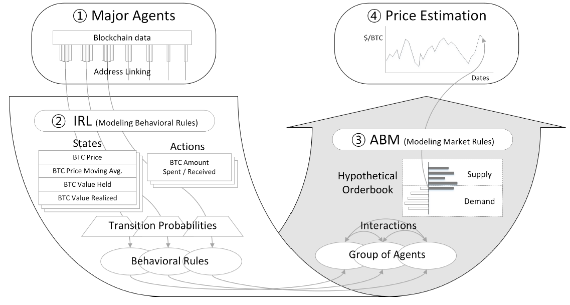
We try to recover the behaviors of each agent from its sequential transactions using an IRL algorithm. We then build an ABM that represents a hypothetical Bitcoin market. Since the market has well-defined interactions, and the supply and demand of the market can be inferred directly from the behavioral rules recovered from the IRL, the ABM is expected to play out over time to predict the future equilibrium prices, at least for a short period of time.
Specifically, the method consists of four steps (numbered 1-4 in Figure 1).
- Identify major agents by address linking
- Model IRL for major agents’ behavioral rules
- Construct ABM for Bitcoin supply/demand
- Predict equilibrium prices for future dates
Identify major agents by address linking
As of Aug. 2017, there are 388 million addresses on the Bitcoin Blockchain. Since typical users have multiple Bitcoin addresses and the transactions are anonymous, it is necessary to group addresses that are controlled by a single entity. This process is called address linking, which itself is an ongoing topic in cryptocurrency research. On this front, we use a method implemented by Kalodner et al. (2017). The heuristics used in this implementation include (1) input addresses used in the same transaction are controlled by the same entity (except for CoinJoin transactions), and (2) change addresses are not reused.
There are 145 million entities (clusters of addresses) identified by the method stated above. Since our model recognizes each entity as an agent, it is simply impossible to run an IRL algorithm for all entities due to its large size. We analyzed the market transaction volume, which reveals that a very small number of agents take up a dominating portion of the whole market. For example, only 18,174 agents make up 65% of the whole market transaction amounts during Jan. 2017 - Jul. 2017. When counting only agents who had more than 30 transactions during the period, only 2,286 agents make up 65% of the counted transaction volume. The shade in the plot below shows agents taking up 90% of market transactions to get a sense of the number of major agents.

Model IRL for major agents’ behavioral rules
An IRL algorithm solves for reward function (\(R\)) with MDP\R which consists of states, actions, and transition probabilities. With \(R\) recovered, we can solve the completed MDP and find an optimal behavioral policy with value iteration. We assume that each agent has its own MDP\R since trading volume is considerably different from agent to agent. Daily transactions of each agent are fed into an IRL algorithm as an observed trajectory of \((s,a)\) pairs. The results of our IRL approach are the (presumably) optimal actions for each state in a given MDP.
A state is defined by four variables: BTC price (\(BP\)), difference between BTC price and moving average of the price (\(PM\)), BTC value possessed (\(VP\)), and BTC value realized (\(VR\)). All values are measured as a daily value based on Coordinated Universal Time (UTC). An agent action (\(A\)) is the net amount of BTC spent on a day. A negative value of action means an agent has net receiving amount on that day. Those variables should be discretized to define discrete states for IRL. In our formulation, the reward discount factor (\(\gamma\)) of the IRL represents a preference for immediate rewards considering market uncertainty and internal rate of return (IRR) of Bitcoin users. The \(\gamma\) is set to 0.9 throughout the method.
Transition probabilities is projected by assuming that daily BTC price change (\(D\)) follows a normal distribution. Any combination of changes in state variables can be calculated by the probability distribution of the price difference since all of the four state variables can be expressed by the daily BTC price change as follows.
| $$\begin{align*}BP_t &= BP_{t-1} + D_t\\ PM_t &= \frac{m-1}{m}\times(PM_{t-1} + D_t)\\ VP_t &= \bigg(\frac{VP_{t-1}}{BP_{t-1}}-A_{t-1}\bigg)\times BP_t\\ VR_t &= VR_{t-1} + A_{t-1}\times BP_{t-1},\end{align*}$$ |
Construct ABM for Bitcoin supply and demand
In order to represent market interactions, we construct a hypothetical order book. Assuming that at a given price level, each agent has its own level of receiving/spending amount that maximizes its long-term goal. The order book provides an efficient way to find the equilibrium price among the participants. Figure 3 below shows the aggregated receiving orders and spending orders of all agents.
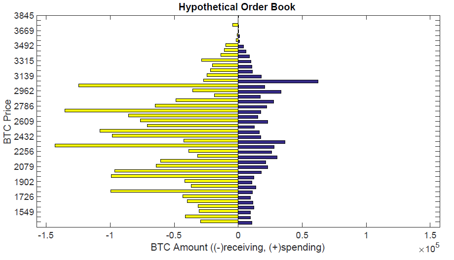
Specifically, it is assumed that agents whose action probability recovered by IRL is greater than .5 are the ones that participate in the market (if two actions have the equal probability, the average of the two actions was used). All participants are assumed to send either a buy order or a sell order with a specific amount. Then, hypothetical transactions are executed at the current price level. When receiving orders or spending orders are left after the executions, the price goes up or down, respectively. If there are only a small number of market participants left, it is assumed that an equilibrium price for the day has been reached. The following figure illustrates how an equilibrium price is found on a given day.
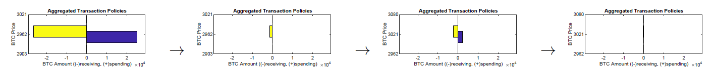
The following algorithm delineates the procedure on a given day.
- First, we set all agents in the simulated market to active, and if there are more than a pre-determined number of agents active in our simulated market we update the BTC moving average, value possessed, and value realized according to the base price price while determining a current state and associated action. We then set the action for the agent.
- Second, based on an agents action as a spender or receiver we determine market equilibrium by matching spenders with receivers until active agents fall below a certain threshold and we reach market equilibrium.
- Lastly, if there is a disequilibrium of spenders and receivers, we adjust the equilibrium price accordingly.

Predict equilibrium prices for future dates
Once an equilibrium price has been found on a given day, the price can play as the next day’s base price on which agents determine their states and associated policies. Thus, the simulation is able to play out for any period of days. Thus, the series of equilibrium prices generated in the simulation is considered prediction prices. While the prediction period is unbounded, the simulation may part ways from the real market trends after several rounds because the cumulative BTC value possessed and BTC value realized by each agent can be different from the real entity even though the predicted price is similar to the real market price.
Experiment and Results
In order to test diverse market conditions, we performed 9 experiments with the proposed method on training data containing different 3-month periods of real Bitcoin transactions ranging from Sep. 2016 to Jul. 2017. Each experiment consists of 100 simulations starting with the same conditions of the last day of training periods. The purpose of the simulation is to obtain percentages of correct directional prediction. A set of 100 simulations gives consistent results when testing multiple trials. The experiments generate equilibrium prices for 12 days, and these prices are compared with the real market prices within the same period.
Dataset
Bitcoin blockchain data was aggregated by summing transaction amounts to generate daily net spent amount by each agent. Training datasets were created for nine 3-month periods starting from September 2016. We used the blockchain data of July 2017 and before to exclude the effect of the hard fork that took place in August 2017. We selected major users that take up 30% of the total market transaction volume. Users who had less than 30 transactions were excluded for training. Both state and action spaces are uniformly discretized for MDP\R by dividing the state space into 50,000 states, 50 for BTC price, 10 for 10-day moving average gap, 10 for BTC value possessed (\(VP\)), and 10 for BTC value realized (\(VR\)). The last price of the training period is set in the middle of the BTC price range to prevent any bias in either direction. The BTC price range is
| $$\begin{align*}\text{from}&: \text{-max(maximum BTC price - last training price, last training price - minimum BTC price)}\\ \text{to}&: \text{max(maximum BTC price - last training price, last training price - minimum BTC price)}\end{align*}$$ |
| $$\begin{align*}\text{from}&: -\frac{\text{|minimum net spending| + |maximum net spending|}}{2}\\ \text{to}&: \frac{\text{|minimum net spending| + |maximum net spending|}}{2}.\end{align*}$$ |
| Training major | Major agents (count) | Last price ($/BTC) | BTC price range ($/BTC) |
| 2016.09 - 2016.11 | 235 | 742.0 | 571 - 912 |
| 2016.10 - 2016.12 | 293 | 968.2 | 609 - 1327 |
| 2016.11 - 2017.01 | 321 | 967.7 | 687 - 1247 |
| 2016.12 - 2017.02 | 346 | 1190.9 | 750 - 1631 |
| 2017.01 - 2017.03 | 295 | 1079.7 | 775 - 1383 |
| 2017.02 - 2017.04 | 253 | 1348.0 | 935 - 1760 |
| 2017.03 - 2017.05 | 260 | 2330.2 | 935 - 3724 |
| 2017.04 - 2017.05 | 272 | 2500.0 | 1089 - 3910 |
| 2017.05 - 2017.07 | 219 | 2873.8 | 1402 - 4345 |
Simulation and validation
Even though we have the exact same behavioral rules for our agents, the market price is determined by how supply and demand are paired. If the market always matches the biggest supply and the biggest demand, the result should be deterministic. However, for a more realistic simulation, we try random matching where the probability of execution is in proportion to the volume. We performed 100 simulations for each of nine periods. The simulation ignored actions of less than 10 BTC, which is usually less than 0.01% of total daily transaction volume. The procedure for finding equilibrium price stops when there are less than 30 active agents left to prevent wavering prices by the last few agents on a day. There are inevitable parameters to model the market with the significantly small number of agents compared to the real market.
Figure 5 below show the 12-day prediction result of the simulations. Because the predicted prices tend to precede the real market prices, the real prices of 10 more days are displayed for a comparative purpose. Since there is no comparable method that utilizes individual data in addition to time-series data, univariate ARIMA model predictions are presented as a baseline, which is most frequently used for time series only data. The price data are clearly non-stationary, and thus we take a first difference of the data for the ARIMA model. The first differencing is compatible with the previous assumption for the transition probability projection. AR and MA orders are chosen with the smallest AIC for each experiment.
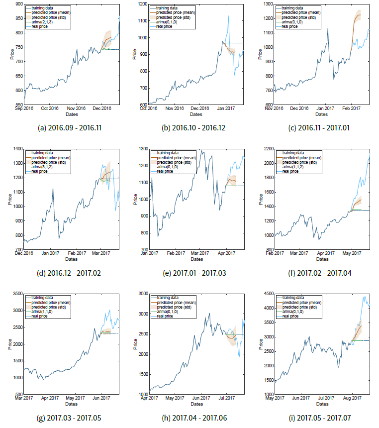
Table 2 shows the percentages of correct predicted direction (up/down) compared to the price of the last training day. The first half of the predictive period tends to be less correct since it does not capture blips of the market prices. However, the prediction rate of the following half-period is almost 80% with the maximum of 85.9% on the 12th day. The prediction rates start to drop after 12 days suggesting that the simulation develops its own direction rather than reflecting the market trend.
The percentage does not represent the accuracy of the prediction. Sometimes, the disparity between the real price and predicted price can be big even though the predicted direction is correct. The predicted prices generated from the simulation model tend to follow the future course of price direction, not necessarily reflecting immediate fluctuation.
| Training Period | Prediction Period | |||||||||||
| day1 | day2 | day3 | day4 | day5 | day6 | day7 | day8 | day9 | day10 | day11 | day12 | |
| 2016.09-2016.11 | 99% | 77% | 93% | 77% | 95% | 97% | 96% | 95% | 96% | 94% | 97% | 98% |
| 2016.10-2016.12 | 0% | 0% | 0% | 0% | 0% | 100% | 100% | 100% | 100% | 100% | 99% | 99% |
| 2016.11-2017.01 | 100% | 100% | 100% | 100% | 100% | 100% | 100% | 100% | 100% | 100% | 100% | 100% |
| 2016.12-2017.02 | 13% | 41% | 48% | 55% | 80% | 78% | 74% | 29% | 72% | 28% | 35% | 72% |
| 2017.01-2017.03 | 100% | 96% | 100% | 100% | 100% | 97% | 92% | 88% | 93% | 91% | 90% | 82% |
| 2017.02-2017.04 | 0% | 47% | 100% | 100% | 100% | 100% | 100% | 100% | 100% | 100% | 100% | 100% |
| 2017.03-2017.05 | 8% | 66% | 78% | 52% | 54% | 63% | 71% | 74% | 70% | 66% | 69% | 60% |
| 2017.04-2017.06 | 71% | 9% | 17% | 16% | 13% | 17% | 16% | 20% | 21% | 75% | 70% | 65% |
| 2017.05-2017.07 | 68% | 16% | 8% | 91% | 92% | 97% | 95% | 93% | 93% | 92% | 94% | 97% |
| Average | 51% | 50.2% | 60.4% | 65.7% | 70.4% | 83.2% | 82.7% | 77.7% | 82.8% | 82.9% | 83.8% | 85.9% |
| ARIMA prediction rate | 33.3% | 55.6% | 55.6% | 44.4% | 44.4% | 33.3% | 44.4% | 55.6% | 44.4% | 44.4% | 44.4% | 33.3 |
Sensitivity analysis
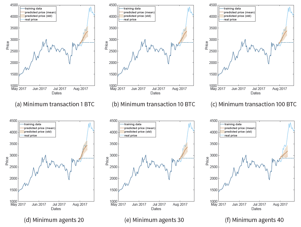
There are not many model parameters since the behavioral rules of agents are generated by IRL. Two arbitrarily chosen parameters in the previous section were (1) minimum transaction amount deciding active agent and (2) minimum number of agents deciding equilibrium price.
We now test these parameters to make sure that they do not affect the result. As shown in Figure 6 below, the minimum transaction amount has a negligible effect on the result. When the minimum number of agents in the market is set to 40 (around 18% of total market participants), the simulation seems to stop running before reaching the equilibrium. When the minimum number of agents is too small, however, the equilibrium price tends to be influenced by the last few remaining agents.
It is worth noting that there is an important parameter that is latent in the IRL state variables: moving average day (m). Since a moving average (MA) smooths out price over m days, it provides a linear trend of the price. We found that m was sensitive to the individual behaviors and thus the following results. When m is small, it does not to provide much additional information since MA acts like price itself. When m is large, it lags the price and does not represent timely decisions of individual users. Since we target 8-12 day, short and mid-term predictions, we decided 10 to be an appropriate value for m.
Discussion
Considering that the market price is the result of interactions of market participants, the reasoning behind our method is straightforward compared to other traditional methods that try to find price movement regularity or secondary correlation between the price and external information. Since our method first builds the market itself with individual participants, we can even trace back the causal chain from the market price to the individuals. Moreover, the use of IRL provides a systematic way to generalize market participants’ behaviors. Since a state-based market model has multitudinous combinations of state variables, it is necessary to project observed behaviors to unobserved states. IRL is an efficient tool for generating behavioral rules in unseen situations (generalization) or even in different model dynamics (transferability). The experimental results indicate that the proposed method could be an effective, new prediction method in the Bitcoin market.
However, several limitations remain. First, our simulations fall short of being able to model a large enough number of agents to simulate more exact real-world scenarios, as one requires too much computational power necessary to run these simulations. We could not perform sensitivity analysis with the number of agents for the same reason. For more accurate simulations, there should be either a faster IRL algorithm or a method to select influential agents. Currently, we only exclude agents with less than 30 transactions, since less than 30 transactions are hard to constitute sequential decisions that are necessary for the IRL method.
A second limitation is that cryptocurrency markets are continually active on a global scale, thus discretizing a day based on UTC is arbitrary. This arbitrariness may result in poor IRL models for some agents and, as a result, a less accurate ABM model. If we can identify each agent’s time zone, we will be able to assign individual time zones. Using a smaller time scale could be another way to circumvent this limitation. Another obstacle we face using this method is that testing multiple parameters in the ABM is not easy since almost all parameters are embedded in the IRL models. This could result in neglecting some important variables in the prediction model.
Conclusion and Future Work
In this paper, we proposed a method for generating synthetic Bitcoin transactions and predicting market prices. We were able to predict short-term Bitcoin price movements by utilizing the motivation-based approach to recover not only exhibited behavioral rules but also unobserved rules rooted in the agents’ motivations. Our results showed a greater than 80% directional predictive accuracy on average after a prediction period of six days. From day 6 to day 12 we encountered our strongest predictive accuracy, displaying our model’s fortitude in predicting short and mid-term price movements in the Bitcoin market.
Our result does not imply that the proposed method outperforms other prediction techniques. The baseline experiment is far from the best effort, and the directional prediction rate is not a fair metric since it cannot measure comparative accuracy and precision of the result. Thus, a follow-up study is necessary in order to show our model’s comparative performance. Since it is not fair to simply compare the results from different datasets and different time frames, the combination of algorithm and dataset should be considered, such as a comparison between IRL+ABM with individual data and other machine learning methods with macroeconomic data.
Once the supply and demand are constructed with ABM, it can be easily expanded to other market behaviors such as price spread, volatility, and trading volume. This expansion can be considered as potential future research, as well as comprehensive validations, since almost all market phenomena can be explained by supply and demand behaviors. Another idea would be understanding market cycles in bear vs. bull trends and how our agents behave during these scenarios. Comparing market movement before and after the Segwit hard fork would be an interesting topic as well.
On the methodology side, we believe that the combination method of IRL and ABM is applicable to much more diverse domains, possibly all areas where ABM is used. By recovering individual rules from data with IRL, this approach can systematically and even automatically build an ABM. In addition, imitation learning is not limited to IRL, and there are a number of techniques that can model behavioral rules from data. One promising future work is applying generative adversarial networks (GANs) in combination with ABM for constructing a predictive model.
References
ABBEEL, P., & Ng, A. Y. (2004, July). Apprenticeship learning via inverse reinforcement learning. In Proceedings of the Twenty-First international conference on Machine learning (p. 1). ACM. [doi:10.1145/1015330.1015430]
AMJAD, M., & Shah, D. (2017, February). Trading Bitcoin and Online Time Series Prediction. In NIPS 2016 Time Series Workshop (pp. 1-15).
COCCO, L. & Marchesi, M. (2016). Modeling and simulation of the economics of mining in the Bitcoin market. PLoS ONE, 11(10), e0164603. [doi:10.1371/journal.pone.0164603]
DVIJOTHAM, K. & Todorov, E. (2010). Inverse optimal control with linearly-solvable MDPS. In Proceedings of the 27th International Conference on Machine Learning (ICML-10), (pp. 335–342)
JANG, H., & Lee, J. (2018). An empirical study on modeling and prediction of Bitcoin prices with Bayesian neural networks based on blockchain information. IEEE Access, 6, 5427-5437. [doi:10.1109/ACCESS.2017.2779181]
KALODNER, H., Goldfeder, S., Chator, A., Möser, M. & Narayanan, A. (2017). BlockSci: Design and applications of a Blockchain analysis platform. arXiv preprint arXiv:1709.02489: https://arxiv.org/abs/1709.02489.
KIM, Y. B., Kim, J. G., Kim, W., Im, J. H., Kim, T. H., Kang, S. J., & Kim, C. H. (2016). Predicting fluctuations in cryptocurrency transactions based on user comments and replies. PLoS ONE, 11(8), e0161197. [doi:10.1371/journal.pone.0161197]
KRISTOUFEK, L. (2015). What are the main drivers of the Bitcoin price? Evidence from Wavelet coherence analysis.PLoS ONE, 10(4), e0123923.
LEE, K., Rucker, M., Scherer, W. T., Beling, P. A., Gerber, M. S., & Kang, H. (2017). Agent-based model construction using inverse reinforcement learning. In Simulation Conference (WSC), 2017 Winter (pp. 1264-1275). IEEE. [doi:10.1109/WSC.2017.8247872]
LEVINE, S., Popovic, Z. & Koltun, V. (2011). Nonlinear inverse reinforcement learning with Gaussian processes. In Advances in Neural Information Processing Systems, (pp. 19–27).
NAKAMOTO, S. (2008). Bitcoin: A peer-to-peer electronic cash system. Accessible at: https://bitcoin.org/bitcoin.pdf.
NG, A. Y., & Russell, S. J. (2000). Algorithms for inverse reinforcement learning. In Proceedings of the 17th International Conference on Machine Learning, (pp. 663-670).
QIAO, Q. & Beling, P. A. (2011). Inverse reinforcement learning with Gaussian process. In American Control Conference (ACC), 2011, (pp. 113–118). IEEE. [doi:10.1109/ACC.2011.5990948]
RAMACHANDRAN, D. & Amir, E. (2007). Bayesian inverse reinforcement learning. In Proceedings of the 20th International Joint Conference on Artificial Intelligence, (pp. 2586–2591)
RUSSELL, S. (1998, July). Learning agents for uncertain environments. In Proceedings of the eleventh annual conference on Computational learning theory (pp. 101-103). ACM. [doi:10.1145/279943.279964]
ZIEBART, B. D., Maas, A. L., Bagnell, J. A. & Dey, A. K. (2008). Maximum entropy inverse reinforcement learning. In Proceedings of The Twenty-third AAAI Conference on Artificial Intelligence, (pp. 1433–1438)