
Introduction
Prediction markets[1] can be described as markets that are “designed specifically for information aggregation and revelation” (Wolfers & Zitzewitz 2004, p. 108)[2]. They are a promising example of using the “wisdom of the crowds” (Surowiecki 2010). The basic idea is to give individuals the possibility to trade their expectations concerning the relevant variable on a virtual market (e.g., the expected number of sales of a product in the next year). Via their trades, the local information of individual actors is aggregated in form of the market price that is visible to all market participants. At the same time, the information of the individual traders is not disclosed to the participants. Prediction markets can be used to reveal and aggregate the diverse information even of large and (geographically) dispersed groups. These characteristics distinguish them from traditional forecasting methods like expert forecasting or statistical methods.
Prediction markets have been applied successfully both in research (Camerer et al. 2016; Dreber et al. 2015; Forsythe et al. 1992) and in practice (Atanasov et al. 2016; Chen & Plott 2002; Cowgill & Zitzewitz 2015). Hewlett Packard (HP) provides a good example for a successful application of prediction markets. HP has used them to project figures associated with the official sales forecast (Chen & Plott 2002). Among the predicted figures were the next month’s revenues for a specific product, the next month’s unit sales of another product and the next quarter’s unit sales. Between 20 and 30 participants traded on a prediction market based on a continuous double auction. The official sales forecast was unknown to the traders. As the prediction market owner, HP was interested in an accurate prediction and offered participants monetary incentives linked to the individual’s success on the market. Compared to the traditional sales forecast, the results of the prediction market were considered a substantial improvement. In six of eight cases, the prediction market outperformed the traditional sales forecast. Additionally, the prediction market correctly indicated the direction of the deviation for all eight cases[3].
A major design question for the set-up of a prediction market is the choice of the market mechanism (Spann & Skiera 2003, p. 1314), i.e. how individuals can trade on the market. It is linked to research about efficient information aggregation in prediction markets and can be seen as a foundational aspect of prediction markets (see Klingert 2017). Different market mechanisms have been applied to prediction markets to coordinate the trading interactions between individual actors. Our work focuses on two of the most common ones – the continuous double auction CDA (e.g. used in the Iowa Electronic Market by Forsythe et al. 1992, p. 1144) and an automated market maker, the logarithmic market scoring rule LMSR (Hanson 2003; e.g. used in the Gates Hillman Prediction Market by Othman & Sandholm 2010a, p. 368).
Present research documents the functioning of prediction markets (Atanasov et al. 2016), but the effects of different market mechanisms on a market’s performance are often sidestepped in this context[4]. The average performance of prediction markets has been “pretty good” (Wolfers & Zitzewitz 2004, p. 119), but some failures to adequately aggregate information have been reported (e.g., Hansen et al. 2004). The fundamentals of prediction markets are sufficiently understood, but the investigation of the forecasting performance is ongoing (Horn et al. 2014, p. 104). The market mechanism is one direction of this research. Field studies of prediction markets (e.g., Forsythe et al. 1992; Hansen et al. 2004; Othman & Sandholm 2010a) have been unable to fully assess the effect of the mechanism because varying it would substantially increase the effort. Furthermore, the market mechanism is often chosen without a thorough discussion or at least without documenting it. Some software providers do not even offer alternative prediction market mechanisms; Crowdworx focuses on the LMSR, for example (Ivanov 2008). Nevertheless, some differences are known. From a technical perspective, the LMSR offers constant liquidity and only requires one trader to execute a transaction while the CDA requires at least two. As a higher number of trades is typically associated with an increase in accuracy, the mechanism choice might be a crucial aspect concerning the performance of a prediction market (Antweiler 2013).
The possible role of the choice of an appropriate market mechanism stands in contrast to the current level of understanding of the effects that different mechanisms have on prediction market outcomes (Healy et al. 2010, p. 1995). While laboratory experiments have focused on a small selection of aspects such as the interplay with the information distribution among traders (Healy et al. 2010; Ledyard, Hanson, & Ishikida 2009), the effects of different environments in conjunction with a specific mechanism are particularly unclear (Healy et al. 2010, p. 1995). Three aspects deserve further attention. First, existing studies do not vary important aspects like the initial money endowment and the actors’ trading strategies (Rothschild & Sethi 2016). Second, some results contradict each other. According to Healy et al. (2010), the accuracy of the LMSR is much lower than the accuracy of the CDA in a simple environment with few traders. This differs from the outcome of an experiment mentioned in a talk by Ledyard[5] referenced in the same paper (Healy et al. 2010, p. 1995) and by Ledyard et al. (Ledyard et al. 2009). The available laboratory experiments (Healy et al. 2010; Ledyard et al. 2009) share the same problem as they rely on a relatively small number of traders (between three and six). An average prediction market has more traders than that[6]. Third, other experimental (Jian & Sami 2012) as well as simulation (Slamka, Skiera, & Spann 2013) studies compare market mechanisms without considering the widely used CDA.
This lack of knowledge concerning the performance effects of the most commonly used market mechanisms is problematic as faulty prediction market outcomes might lead to wrong decisions. Due to the increased popularity of prediction markets in the corporate context (Bray, Croxson, & Dutton 2008, p. 6), the relevance of differences between mechanisms has risen further. Corporate prediction markets might also face specific conditions that can affect the performance of the market mechanism (Cowgill & Zitzewitz 2015). For example, the number of traders might be limited in corporate internal markets. Consequently, the decision of traders with limited skill in stock market trading might have more weight than in large prediction markets (Rothschild & Sethi 2016). Therefore, random strategies might represent some traders better than other strategies (Cowgill & Zitzewitz 2015), for example, a strategy based on the expected value.
Against this backdrop, our paper provides a comparative analysis of the CDA and the LMSR concerning relevant prediction market output variables like number of trades, standard deviation of the price and accuracy level[7]. It contributes to understanding the mechanism-related effects and the dynamics of the collective information aggregation of the participants by introducing and analyzing an agent-based simulation model. It follows an iterative process to establish strong links with economic laboratory experiments (Klingert & Meyer 2012a) and it is based on a laboratory experiment, i.e. the simulation model is constructed and micro as well as macro validated using the experimental data of Hanson et al. (2006). We also aim at providing input for future laboratory experiments by identifying aspects that warrant further investigation. Our results underline the impact of the mechanism selection. Due to the higher number of trades and the lower standard deviation of the price, the LMSR seems to have a clear advantage at a first glance. However, considering the accuracy level as independent variable, shows that the effects are actually more complex and depend on the environment and actors.
The paper is structured as follows. First, a review of relevant literature is provided and the hypotheses for the simulation experiments are derived. Second, the simulation model is introduced. Third, the model is micro as well as macro validated. Fourth, simulation experiments are conducted, analyzed and tested for robustness. The paper concludes with a discussion of the results and a brief outlook.
Literature Review and Hypothesis Development
This paper provides a comparative analysis of the CDA and the LMSR. The CDA has traditionally been the standard prediction market mechanism (Chen & Pennock 2010). Like on many financial markets, two traders directly exchange stocks and monetary units as it is illustrated in Figure 1. Asks and bids are placed in an order book and can subsequently be accepted by other traders. If an ask or bid is accepted, stocks and monetary units are exchanged and it is deleted from the order book.

Contrary to the CDA, an automated market maker serves as the trading partner for each type of trade in the LMSR (see Figure 2). It offers to buy and sell at a certain price. Therefore, the actors can only accept the given prices or do nothing. The prices are calculated based on a logarithmic function (for details see Pennock & Sami 2007, pp. 663-664) enabling the LMSR to act like an “intermediary between people who prefer to trade at different times” (Hanson 2009, p. 61). A loss of the market maker is accepted in such prediction markets, and has to be covered by the market owner, but unlimited losses are not incurred (Hanson 2009, p. 62).
Ken Kittlitz, Chief Technology Officer at the software provider Consensus Point, points out important differences between the two market mechanisms:
"Having run markets both with and without Hanson‘s automated-market maker [LMSR], we say with confidence that it makes a huge difference to the success of the market. Because it maintains buy and sell orders at a wide range of prices, it provides a steady source of liquidity that would otherwise be lacking. This allows traders to interact with the system in an easy and intuitive manner rather than having to worry about placing booked orders at certain prices and waiting for other traders to match those orders." (cited in Hanson 2009, p. 62)
In this section, we will break several of his field observations down into testable hypotheses. To this end, first, we define criteria for the evaluation of the market mechanisms. Then, we draw upon prior research and the technical differences between the two mechanisms to derive our hypotheses.
Concerning related research it is important to mention the study by Brahma et al. (2012). They compare a recently suggested liquidity-sensitive variant of the LMSR (LS LMSR) with a Bayesian Market Maker. Their paper provides many useful insights in the LMSR – e.g., the amount of loss incurred in such markets – and can be seen as complementary to this study, because it does not address the CDA. Still, the methodological approaches slightly differ, as our paper is validated based on a laboratory experiment, wants to explore parameter values and combinations not explored in this experiment and finally to guide future laboratory experiments (Klingert & Meyer 2012a). Brahma et al. (2012) use laboratory studies as an additional way to evaluate their Bayesian Market Maker in comparison to the LMSR.
The prediction market mechanisms will be assessed based on three evaluation criteria. The first criterion is the quantity of trades, because the number of trades is important for the success of a market. An increase in the number of trades offers the opportunity to add more pieces of information to the market price. The second criterion is accuracy and is measured by the accuracy level. According to Hanson et al. (2006), it represents a key figure and mainly determines the quality of a prediction market. The accuracy level is more important than the number of trades because a higher number of trades does not necessarily lead to a high predictive quality, e.g., when traders act randomly. The accuracy level is defined as the variance between the price and the correct value (Hanson et al. 2006, p. 456). The third criterion is the standard deviation of the price (e.g., used by Jian & Sami 2012). It measures reliability and assumes that a good average accuracy might still not be sufficient in itself. Because extreme predictions might have severe consequences, it is important to be aware of them. A substantial reduction of price variation can even make a slight reduction of the average accuracy acceptable.
Data to assess the three criteria is collected after the prediction market closes. The accuracy level represents the most important measure of prediction market quality. Because the accuracy is expected to only partially depend on the mechanism, interaction effects with other variables are considered. Besides, the number of trades and the standard deviation of the price are explored. While we expect the insights regarding these two criteria to be less complex, their analysis further contributes to the model validation[8].
The first hypothesis addresses the number of trades. From a technical perspective it seems quite straightforward, that the LMSR has an advantage in achieving a higher number of trades. The CDA needs at least two traders to execute a trade whereas the LMSR provides constant liquidity and should be able to act like the second trader. Still one can consider situations, in which the LMSR has less trades compared to the CDA. The LMSR has a certain spread between the prices to sell and buy which can lead to no trades in the presence of traders willing to trade for prices within this spread. Contrary in CDA, the spread is defined by the orders in the order book and can be smaller. Still, the advantage of the LMSR concerning an increased number of trades has been observed in the field. Ken Kittlitz has noted that the “number of trades in a market using the market maker is at least an order of magnitude higher than in one not using it” (cited in Hanson 2009, p. 62). In contrast, prediction markets with the CDA may suffer from low liquidity which leads to manual interventions of market owners (Antweiler 2013; Chen & Plott 2002, p. 10). Therefore, the first hypothesis is formulated:
Hypothesis 1: The LMSR has a higher number of trades than the CDA.
The second criterion is accuracy. It is central to prediction markets as the accuracy level measures the quality of the prediction market result, but stating a hypothesis for or against one of the mechanisms is less intuitive. Because the LMSR was introduced after the CDA and specifically addresses some of its problems, it might be seen as favorable. The following aspect in particular could be seen as a distinct advantage of the LMSR. Trades are needed to incorporate the information of the agents and a higher number of trades is typically related to an increased accuracy. However, most properties of the mechanisms have two sides. Having a market maker (LMSR) might be beneficial, if no trades are expected with very few traders. In the absence of no trades and assuming an early end of the market, the trade volume might be too low to achieve an accurate value when using the LMSR. The market maker requires certain minimum volume to adjust the price. The CDA is able to change the price with the trade of a single stock. Empirical research does not give a clear direction in this regard because two parallel prediction markets to directly compare the CDA and the LMSR are hardly implemented. Currently, the LMSR is the standard market maker mechanism used at several companies including Inkling Markets, Microsoft and Yahoo (Chen & Pennock 2010). One may assume that the LMSR’s accuracy is a driver of its success. It might come as a surprise that the experimental literature paints a different picture. According to Healy et al. (2010), the accuracy of the LMSR is much lower than the accuracy of the CDA in a simple environment with few traders. Their results are not consistent with the outcomes of other experiments, e.g., an experiment mentioned in a talk of Ledyard et al. (2009) referenced in the same paper (Healy et al. 2010, p. 1995). Overall, the LMSR is supposed to be the slightly superior mechanism considering its positive reception due to the enhanced liquidity and the slight advantage for the LMSR in the experimental studies. This leads to our second hypothesis:
Hypothesis 2: The LMSR is more accurate than the CDA.
We augment this perspective on accuracy and add two sub-hypotheses to address potential interaction effects for three reasons. First, the technical differences regarding this research question do not give a clear direction regarding the effect of the market mechanism on accuracy. Second, literature does not suggest a clear direction too. Third, the accuracy level can be regarded as the most important criterion.
Hypothesis 2a addresses the presence of random strategies. We study this, because some participants in a prediction market might not be trained stock traders. The LMSR is supposed to be superior in this case for several reasons. The LMSR restricts the action space more than the CDA and, thus, traders have fewer options. The LMSR also requires less sophisticated strategies, because the size of the action space is stable and the acceptance of asks and bids is more certain. Healy et al. (2010, p. 1979) claim that confused traders could influence both, the CDA and the LMSR, and do not determine a clear advantage for one of the mechanisms. We follow the theoretical considerations with our hypothesis 2a:
Hypothesis 2a: The LMSR is more accurate in the presence of random strategies than the CDA.
Hypothesis 2b addresses “extreme information distributions”. Extreme information distributions reflect a correct value at the border of the possible states. If 0, 40 and 100 are the possible states, information distributions with the correct value 0 and 100 are considered as “extreme”. Extreme states can be very relevant in practical settings. The CDA is supposed to have an advantage over the LMSR, because it has a broader action space which enables traders to achieve large price movements with low trade liquidity. The LMSR requires the traders to bet against the liquidity of the market maker first which prevents them from immediately moving the price to an extreme value.
Hypothesis 2b: The CDA is more accurate for “extreme information distributions” than the LMSR.
The third criterion is the standard deviation of the final price. It can be an important measure for applications because it reflects the reliability of a prediction market. A high probability of a small deviation might be more acceptable than a low probability of a high deviation if the latter results in a disastrous decision. The LMSR can be expected to have a lower standard deviation because of the restricted action space for traders. Furthermore, the traders can only choose from three actions at any given time: they can accept to buy from the market maker, sell to the market maker or do nothing. Furthermore, the prices of the market maker direct the trading and the liquidity prevents fast price changes. Therefore, extreme trades do not immediately result in extreme deviations from the correct value. Still, the empirical literature is contradictory in this regard. Healy et al. (2010, p. 1988) report a higher variability in the distance between output and correct result for the LMSR. However, they are not reporting the exact standard deviation and their results are at odds with their theoretical considerations. Overall, we follow the theoretical considerations with our third hypothesis:
Hypothesis 3: The LMSR has a lower standard deviation of the final price than the CDA.
Simulation Model
The purpose of the agent-based simulation model is to analyze the effect of the two mechanisms on the number of trades, the accuracy of results and their reliability. A simulation model is applied to analyze the effects of interest, because prediction markets are markets from a technical point of view and, as such, a complex system (see Tseng et al. 2009). The collective process of information aggregation is rather difficult to predict because the price is as much influenced by traders as they might be influenced by the price themselves. Furthermore, changing the sequence of otherwise identical trades might yield different outcomes. We use an experiment-based simulation to analyze the influence of different factors including relationships that can hardly be controlled and detangled in reality like e.g., the heterogeneous strategies of actors which have been observed in real prediction markets (Rothschild & Sethi 2016).
Using a simulation model to complement existing economic laboratory experiments has at least two advantages (for a more detailed comparison of simulation and laboratory experiments see Klingert & Meyer 2012a). First, actor strategies can be controlled and, therefore, intentionally manipulated. Second, simulation experiments can be executed more efficiently which enables a much broader experimental design including up to 7 factors and 100 simulation runs for each factor combination. The simulation itself benefits from the strong link to laboratory experiments because outcomes of the default model are validated and strategies are chosen by classification based on experimental data. In this section, only an excerpt of the model description and model design considerations can be given due to space limitations. A more detailed documentation based on the ODD protocol (Grimm et al. 2010) can be found in Klingert (2013)[9].
We have chosen the well-documented and influential laboratory experiment of Hanson et al. (2006) as the starting point. The authors gave us access to their experimental data, which allowed us to micro and macro validate the model. Consequently, the default setting of our simulation model strongly resembles their experiment[10]. Twelve agents are initially presented with 200 monetary units and 2 stocks. Both stocks grant the right to receive a payoff of 0, 40 or 100 with equal probability at the end of the trading period. The agents know individually that one value can be excluded with certainty from the possible outcomes. If the true value is 40, half of the agents know it is not 0 and half of the agents know it is not 100, for example. Therefore, an agent, which can dismiss 0 as the true value, knows that the true value is either 40 or 100 and that the stock has an expected value of 70.
The simulation and the experiment differ only slightly in their procedure. One of the differences is that the simulation model is executed stepwise instead of the continuous flow of time in the experiment of Hanson et al. (2006). Every CDA-based step allows the agents to place a bid or ask limited to the natural numbers between [0, 100]. Alternatively, they can accept an order from the order book. If an offer is accepted, the trade is executed and money and stocks are exchanged. The agent order is determined randomly to align the simulation with the laboratory experiment[11]. After the simulation ends with completing step 60, it shows a comparable number of trades (0-41 trades instead of 8-37) to the laboratory experiment which lasts 5 minutes (Hanson et al. 2006, p. 451). Consistent with other market simulations (Gode & Sunder 1993, p. 122), the agents are limited to trade one stock per step and the unmatched offers are deleted after a trade to simplify the decision-making; the agents are allowed to place the same offer in the next step.
To compare market mechanisms, the simulation model goes beyond the laboratory experiment and is varied along the environment and the agents[12]. The market institution is defined by its rules, i.e. the market mechanism. The CDA and the LMSR are used in the simulation experiments. The implementation of the LMSR demands a concrete b-value which determines the maximum loss of the market maker[13]. To achieve a comparable result for the CDA and the LMSR, the b-value of the LMSR should be linked to the CDA setup. The maximum costs of the CDA equal the initial endowment of money and the value of the initial stocks per agent. Given a certain correct value in CDA, these costs are always constant, and therefore the maximum costs equal the minimum costs independent from the market outcome. In LMSR, the agents are endowed with 200 monetary units as well. Contrary to CDA, they are not holding any stocks at the beginning. This is unnecessary because each trade is executed with the market maker as a trading partner. Instead, the b-value is chosen in a way that the maximum loss of the market maker is comparable to the costs of a market based on a CDA[14]. This ensures a fair comparison of both mechanisms.
The environment is mainly defined by the information distribution. The standard task is to predict a state out of the three possible states 0, 40 and 100 (as in Hanson et al. 2006). In each of the states, 50% of the agents know that one of the wrong values is not the true state and the other 50% know that the other wrong value is not the true state. The information distributed among all agents can be considered as complete and certain as the exact value could be easily determined, if the information of all agents was publicly available. Each individual agent has incomplete, but partly certain information because one of the states can be excluded with a certainty of 100%. In addition, other information distributions are chosen to test the robustness of the results.
Finally, the agents trade based on simple rules. The “family” of zero intelligence[15] (ZI) traders is used because these strategies fulfill four criteria. First, the zero intelligence agents have been used in a large number of market simulations (Chen 2012), which also allows for relating our results to previous research. Second, the simplicity of the zero intelligence traders allows for focusing on the influence of the market mechanism in the model. Third, the zero intelligence agents have already been validated at the macro level by prior research that has recognized similar efficiency levels for markets with ZI traders and markets with human traders (Gode & Sunder 1993, p. 133). Therefore, zero intelligence agents seem to be appropriate to direct subsequent experiments. Fourth, strategies that can be validated at the micro level[16] are desirable. The zero intelligence strategies have not been micro validated statistically in the original papers (e.g., Gode & Sunder 1993)[17]. However, the simplicity of the zero intelligence strategies allows for statistical micro validation (see Appendix).
The verification (cf. Gilbert & Troitzsch 2005, p. 19) of the model relies on three basic procedures: The model is based on (semi-)formalized models, it was tested several times and the code was inspected by a step-by-step debugging.
The validity of our model is ensured in three ways with a particular focus on the strategies of the agents. First, the model setting is almost identical to the laboratory experiment of Hanson et al. (2006) as discussed in the previous section. Second, the experimental micro data from Hanson et al. (2006) informed the strategy selection[18]. Third, a macro validation is performed. Gode and Sunder (1993) already compared the results of ZI-agents with data from laboratory experiments at the macro level in their foundational publication. Adding to that comparison, a macro validation based on the experimental data from Hanson et al. (2006) will be discussed briefly.
The experimental micro data from the laboratory experiment of Hanson et al. (2006) provide the starting point for selecting the agents’ strategies. In this work, the micro validation does not aim at showing human traders behave exactly like ZI-traders. Instead, the ZI-strategies are only tested for a best fit at the micro level. While comparisons between the ZI-agents and macro data from laboratory experiments exist (e.g. in Gode & Sunder 1993), a micro validation has not been performed yet.
In general, strategies can be validated at the micro level with a variety of methods like classification, calibration or clustering. Classification starts with a pre-selection of certain agent strategies on a theoretical basis and assigns the actors to the strategies (see Kantardzic 2003, p. 2). Calibration goes beyond classification by adapting the strategies, e.g., by choosing certain parameter values, to better represent the actions of the actors (see Boero & Squazzoni 2005). Clustering does not start with classes, but tries to identify groups in the behavior of the actors instead and defines strategies with the best fit for these groups (see Kantardzic 2003, p. 2).
The purpose of the simulation determined our choice of classification as validation method. We aim neither at prediction nor at pure replication, but at explaining and going beyond the setup of the laboratory experiment. Furthermore, the mechanism rather than the agent behavior represents the research focus. Classification does not adapt strategies or develop new strategies and, thus, offers at least three main advantages over the other two validation methods. First, the attributes of classification potentially reduce the problem of overfitting (Kantardzic 2003, p. 74) present in calibration techniques[19]. Second, it allows for selecting from a pool of strategies that were applied and tested by prior research. Third, keeping the strategies simple from a theoretical perspective allows for focusing on the mechanisms. Overall, these advantages do not only ensure that the strategies are suitable for the experimental setup they are validated for, but also enable simulation experiments to go beyond the laboratory experiment.
Overall, as a result of our micro validation, homogenous and heterogeneous models are selected (see Appendix for details). Two homogenous models, i.e., models where all traders are following the same strategy, are suggested based on the micro validation. First, fundamental trading is represented by ZI.EV traders. The ZI.EV traders (derivation from ZIC, see Gode and Sunder 1993) and N-ZI (Duffy and Ünver 2006) are selling above and buying below the expected value (exact price is chosen randomly with a uniform distribution like in Gode and Sunder (1993). Second, a mix between fundamental and trend trading is implemented via N-ZI traders (Duffy and Ünver 2006). These traders weight the expected value and the last price to select when to buy and to sell.
The list is extended by a learning model. These zero intelligence plus traders (ZIP) (ZIP, Cliff & Bruten 1997) adapt a profit margin based on the success of the last trades and only have a small price span in which they trade. This model has not been micro validated due to the complexity which results from the learning model’s memory and its ability to adapt to its environment. The ZIP agents are used, because they are an instance of the zero intelligence family as well as a learning strategy. For micro validation, zero intelligence unconstraint traders (ZIU) are used as a benchmark model. ZIU traders (ZIU, Gode & Sunder 1993) randomly decide to buy or sell and at what price. This is the trading strategy from the original paper by Gode and Sunder (1993).
Finally, heterogeneous models containing agents with different strategies are added to the list in Table 1. While both the default and the alternative model assume one strategy for all agents, heterogeneous models combine two pure strategies. Furthermore, heterogeneous models consider information distribution and contain at least two agents for each strategy[20]. Mix 1 considers the equal division of the actors and is restricted by a balanced information distribution to outweigh the ZI.EV strategy. It comprises the two strategies derived from the validation without the ZIU strategy. Therefore, the heterogeneous model Mix 1 can be seen as a “lower boundary” of random traders. The heterogeneous model Mix 2 contains the two strategies derived from the validation as well as the ZIU strategy given that the ZIU strategy could not be rejected for 12 actors in the combinatorial case. Therefore, it represents the idea of an “upper border” of random traders.
| No. | Model name | Strategy used | Strategy distr. (12 agents) |
| 1 | Default | ZI.EV | 12 ZI.EV |
| 2 | Alternative | N-ZI | 12 N-ZI |
| 3 | Mix 1 | ZI.EV, N-ZI | 8 ZI.EV, 4 N-ZI |
| 4 | Mix 2 | ZI.EV, N-ZI, ZIU | 4 ZI.EV, 4 N-ZI, 4 ZIU |
| 5 | Learning model | ZIP | 12 ZIP |
The model is also macro validated (see Klingert 2013), even though market outcomes with zero intelligence agents have already been compared with macro data in the past (Gode & Sunder 1993). Comparing the stylized model results from different strategy combinations with the empirical results of Hanson et al. (2006) leads to similar patterns or stylized facts at the macro level (see also Grimm et al. 2005; Heine, Meyer, & Strangfeld 2005). For example, a similar average accuracy for ZI.EV, N-ZI traders and the Mix 1 model can be observed[21]. Mix 2 with random traders and the learning model ZIP yields a lower average accuracy. However, it is superior in rebuilding the distribution of the accuracy level and can be seen as an upper boundary of randomness. As the learning model, ZIP represents a different group of strategies. Therefore, all strategy combinations (besides the model where all traders are following the fully random ZIU strategy) are included in the model.
Experimental Design, Results and Robustness Tests
In this section, the experimental design and results as well as tests for robustness are described. Using an experimental design for multi-agent models has several advantages (see Lorscheid, Heine, & Meyer 2012 for more detailed explanations and further literature). First, it provides a very economical and effective way to communicate the way we analyzed the behavior of our model and the results of these experiments. Looking at the factors one can see which model parameter are varied during our simulations experiments and with which values. Table 2 shows the factors (see second column “factors”) that are varied in a 3k-experimental design, i.e. an experimental design with 3 factor levels per ratio-scaled variable (see the columns “low”, “default” and “high”). Second, it avoids the problem of sensitivity analyses, which vary only one parameter at a time, and allows for the systematic detection of interaction effects. The 3k- is chosen over a 2k-experimental design because it allows for choosing the low and high values linearly around the default value and, thus, systemizes the analysis of results. Furthermore, it allows for the identification of possible non-linear effects (Law 2014; Lorscheid et al. 2012).
| Scale | Factors | Low | Default | High |
| Nominal | Mechanism | CDA, LMSR | ||
| Strategy | ZI.EV, N-ZI, Mix 1, Mix 2, ZIP | |||
| Information distribution | CV 0[22], CV 40, CV 100 | |||
| Ratio | Steps | 30 | 60 | 90 |
| Number of agents | 6 | 12 | 18 | |
| Initial stocks | 1 | 2 | 3 | |
| Initial money | 100 | 200 | 300 |
As the model is predominantly validated based on the experiment of Hanson et al. (2006), the default factor levels are selected accordingly. The simulation ends after 60 steps to represent the 5 minutes of the experiment. Like in the experiment, 12 agents receive an initial endowment of 2 stocks and 200 monetary units. The CDA represents the default mechanism both in the simulation and in the experiment. The default strategy is the ZI.EV strategy as it best represents the actors in the micro validation when comparing pure strategies. The information distribution is aligned with Hanson et al. (2006) as well. In assigning the same probability to the possible values 0, 40 and 100, 50 % (50 %) of the agents know that the true value is not 0 (100).
The analysis in the following section is carried out from different perspectives. After introducing the simulation results by means of an exemplary simulation, the results are documented along the three evaluation criteria (cf. Kleijnen 2015; Lorscheid et al. 2012). First, each hypothesis is tested comparing the averages of 100 runs[23] that are based on the default setting. Second, further tests are performed including the comparison of the averages over all factor combinations and for each of the factor combinations in the experimental design. Third, an overview of the effect sizes of main and 2-way-interaction effects is given. The presentation of the ANOVA results focus on effect sizes rather than on statistical significance, as for most factors the latter is much less important in simulation experiments (Troitzsch 2014). This is driven by very small p-values for the majority of factors that result from the experimental design, which involves 100 simulation runs per factor combination (Secchi & Seri 2016). Partial η2 is chosen as the effect size measure[24] to balance the influence of the factors and the size of the error. Therewith, this measure documents the effect of a certain treatment. If a treatment has a higher effect size compared to other treatments, its influence on the dependent variable can be considered as more important. Finally, the results are tested for robustness from two further perspectives: environments assuming extreme factor levels and assuming different information distributions.
Exemplary simulation runs
Figure 3 shows one exemplary simulation run for each mechanism. It depicts the prices for both mechanisms for all 60 steps within the default setup.
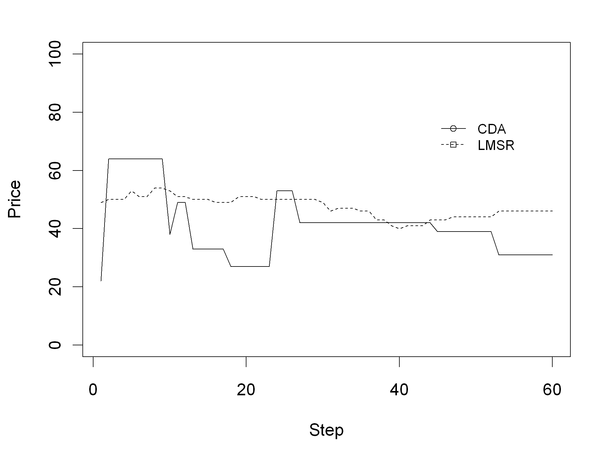
Figure 3 also indicates that clear differences exist between the CDA and the LMSR regarding the price development. While the price changes are small under the LMSR (maximum difference of 3 monetary units between steps), the price changes under the CDA reach up to 42 monetary units. Furthermore, the number of price changes is higher for the LMSR (33) than for the CDA (10). Even though they are exemplary, the two simulation runs already give first indications concerning H1 and H3.
To obtain a clearer sense of the reliability of these first observations, Figure 4 summarizes 200 rather than 2 runs. There is some indication of a lower standard deviation in LMSR. The boxes are clearly smaller in LMSR than in CDA. However, the figure only reflects the results of one parameter combination. The results might not be robust in different settings of the simulation model. Therefore, they are tested with different factor combinations subsequently.

Number of trades
Results displayed in Table 3 offer strong support for hypothesis 1. The first column gives the averages of 100 runs per mechanism in the default setting. The LMSR has a clear advantage and achieves an average of more than three times the trades compared to the CDA. This result in the default setting is highly statistically significant. The second column shows the averages of 121,500 runs per mechanism over all possible combinations. Again, the advantage of the LMSR is obvious. The CDA achieves more trades than in the default setting on average, but the LMSR still results in nearly twice the number of trades. The third column compares the averages of 100 runs per mechanism in each of the 1,215 factorial combinations. If the CDA has more trades than the LMSR for a certain setting, it is counted as a winning setting for the CDA. The case is counted against the hypothesis for equal averages. The LMSR is superior to the CDA once more. In 1,108 factorial combinations (88.07%) the LMSR has more trades than the CDA.
| Default setting | All settings | ||
| Mean trades | Mean trades | Win. settings | |
| CDA | 10.70 | 16.76 | 107 |
| LMSR | 34.95*** | 32.62*** | 1108*** |
Interestingly, the LMSR does not perform better in every setting. The majority of the cases against the hypothesis, which signalize an advantage of the CDA, are driven by the ZIP-strategy (93 of 107 factorial combinations are ZIP settings). Agents applying the ZIP strategy learn a price range. This range might be too small to move the given prices of the LMSR, but it can be sufficient to exchange stocks at a constant price over a longer time period[25]. Thus, the CDA has an advantage in these cases. A reason for the higher number of trades in LMSR in most of the other cases could be that the LMSR provides steady liquidity and, therefore, an execution of a trade is always possible. Assuming there is only one ask and one bid, the CDA results in a maximum of one trade while the maximum in the LMSR is two.
Overall, the mechanism induced effects on the number of trades are strong and the LMSR is superior in achieving a high number of trades.
To understand the importance of the influence of the market mechanism compared to other factors varied in the experiment, an analysis of variance (ANOVA) is conducted over all settings. The main effect “market mechanism” emerges as the third largest effect (.526) in an ANOVA including all main and interaction effects. Only the main effects “agent strategies” (.752) and “number of agents” (.689) have a higher effect size. This shows that changing the market mechanism is a decision that considerably affects the number of trades. The agent strategies and the number of agents result in an even higher effect size due to the increased number of trades in the presence of certain traders, for example, random traders. However, the higher number of trades triggered by random traders might not necessarily improve accuracy. Finally, the R2 is relatively high at .917 and outlines that the influence of random effects is rather low and that it is easy to influence the number of trades by intentionally adapting the identified factors, for example, by choosing the LMSR instead of the CDA.
Accuracy level
In this subsection, the effects on the accuracy level (hypothesis 2 incl. sub-hypothesis) are analyzed. Hypothesis 2 has to be declined, because the expected advantage of the LMSR is not consistent (see Table 4). Like in Table 3, the first column shows the averages of 100 runs per mechanism in the default setting. The default setting replicated from the laboratory experiment results in an advantage for the LMSR with a mean accuracy level of 110.13 vs. 224.17 for the CDA and, thus, supports the hypothesis. The second column gives the averages of 121,500 runs per mechanism over all possible combinations and suggests a different outcome. The mean over all settings documents a slight advantage for the CDA. The high number of simulation runs makes this result statistically significant too, but the difference of less than 3% can be considered as small. The third column compares the averages of 100 runs per mechanism in each of the 1,215 factorial combinations. This comparison further underlines the lack of a clear direction because both mechanisms appear superior in about the same number of settings. An exact binomial test shows that the difference is not statistically significant assuming each of the mechanisms to be superior with a probability of 50%. The results indicate the need for a more detailed analysis.
| Fixed values | Default setting | All settings | ||
| Mean trades | Mean trades | Win. settings | ||
| Default | CDA | 224.17 | 1,326.82*** | 630 |
| (none) | LMSR | 110.13*** | 1,361.29 | 585 |
To guide this analysis we again conducted an ANOVA, which helped us to identify important interaction effects (Lorscheid et al. 2012). Among the most important interaction effects denoted in Table 5 is the “market mechanism”. Therefore, the interaction effects of the mechanism on the accuracy level have to be analyzed too in order to gain a comprehensive understanding. Interestingly, the main effect is relatively small and the influence of the market mechanism is only observed in relation with other effects. The interaction effect with the information distribution is much higher, for example. Other effects result from an interaction with the initial endowment of money and the simulation step. However, the information distribution is the most important effect and more than ten times larger than the highest effect size including the “market mechanism”. The main effect “agent strategy” represents the second most important effect after the information distribution[26]. While the N-ZI traders are achieving the best results with an average accuracy level of 1187.65 over all settings, the prediction market with the Mix 2 model is significantly worse with an average accuracy level of 1680.94. ZI.EV traders (average accuracy level of 1209.28) and the Mix 1 model (1212.54) are nearby the result of the N-ZI traders. ZIP traders are ranging in between (1429.85). This also documents the relevance of a non-arbitrary selection of strategies, for example, by comparing them with experimental data.
| Effect sizes Accuracy level | Simulation step | Information distribution | Market mechanism | Number of agents | Initial stocks | Agent strategies | Initial money |
| Simulation step | .003 | .003 | .003 | .000 | .000 | .009 | .000 |
| Information distribution | .552 | .020 | .002 | .004 | .015 | .013 | |
| Market mechanism | .001 | .002 | .001 | .033 | .008 | ||
| Number of agents | .000 | .000 | .003 | .000 | |||
| Initial stocks | .000 | .000 | .000 | ||||
| Agent strategies | .068 | .002 | |||||
| Initial money | .005 |
With the independent variable “accuracy level“, the R2 is lower than the R2 regarding the number of trades indicating a higher impact of randomness on the accuracy level. Therefore, influencing accuracy seems to be less straightforward than influencing the number of trades. The information distribution is not only an important but also a less complex decisive factor. One could argue that the information distribution of Hanson et al. (2006) is extreme and that other information distributions might impact the result less. Nevertheless, the main effect caused by the information distribution can be seen as dominating the other effects. Therefore, the hypothesis will be further tested for other information distributions in the robustness subsection.
The same three comparisons are made again to analyze the sub-hypotheses to analyze some of the interaction effects in more detail. The mean accuracy level in the default value is compared between the two mechanisms. Both, the mean accuracy level over all settings and the mean accuracy level for each setting of the full factorial design is assessed (see Table 6). One of the values is fixed in Table 6 to cover the sub-hypothesis and the analysis therewith differs from the analysis of the default model. For example, the fixed value “Strategy: Mix 2” means that the Mix 2 strategy combination is considered instead of the ZI.EV traders to analyze hypothesis 2a.
| Fixed values | Default setting | All settings | ||
| Mean trades | Mean trades | Win. settings | ||
| Strategy: | CDA | 639.95 | 1,920.93 | 32 |
| Mix2 | LMSR | 113.90*** | 1,440.95*** | 211*** |
| Knowl.: | CDA | 1,321.75*** | 1,732.83*** | 290*** |
| CV0 | LMSR | 1,792.71 | 1,941.43 | 115 |
| Knowl.: | CDA | 1,691.58** | 1,880.51*** | 267*** |
| CV100 | LMSR | 1,849.50 | 2023.47 | 138 |
Hypothesis 2a is supported and states that the LMSR is superior in the presence of fully random traders (ZIU). Table 6 shows that the mean accuracy level both in the default and over all settings is significantly better for the LMSR assuming a strategy distribution Mix 2 (with ZI.EV, N-ZI and ZIU traders). This result holds for 86.83% of the settings. The stability of the LMSR could explain the improved accuracy level because ZIU traders potentially lead to bigger changes in the CDA. The LMSR does not prevent wrong trades, but lowers the maximum influence of each trade on the price.
Hypothesis 2b is also supported and claims that the CDA is superior for extreme information distributions, i.e. information distributions at the border of the possible states. As documented in Table 6, the CDA is superior to the LMSR for a correct value of 0 and 100 respectively[27]. Over all settings, the CDA achieves a better result in more than 65% of the cases. The importance of the initial liquidity in the LMSR can be seen as a reason for this. The money is always owned by the traders in the CDA while both the market maker and the traders own money in the LMSR. For example, the average amount of money held by the traders is always equal to the initial endowment of 200 with a correct value of 100 after 60 steps in the default model based on the CDA. This money is not distributed equally between the traders; however, most traders are still able to participate in trading. The traders hold on average 256.19 monetary units (information: correct value is not 40) and 143.81 respectively (information: correct value is not 0) after 60 steps. Therefore, both groups have on average more than 100 monetary units per trader and, therefore, are theoretically able to push the price up to 100. The LMSR yields different outcomes. The market maker is holding part of the money while the traders hold additional stocks. Therefore, the average amount of money is reduced to 143.42 (information: correct value is not 40) and 80.25 respectively[28] (information: correct value is not 0). Having an average of 80.25 monetary units already detains the average trader in the second group from increasing the price to 100. Taking into account, that the minimum final endowment of 16 monetary units in the LMSR mostly prevents the agent from trading, shows that the CDA has an advantage with extreme information distributions of keeping the money in the market. With an initial endowment of 300, the disadvantage of LMSR is reduced. The CDA only slightly profits from more liquidity (CV0: 1318.79 and CV100: 1683.06), but the average accuracy level with the LMSR is clearly improved (CV0: 1617.84 and CV 1737.65) compared to the lower initial endowment as presented in Table 6. The better accuracy can be explained by an increased average money endowment at the end of the trading. While the traders in the CDA have an average amount of 300 monetary units, it is again lower in LMSR (196.19). However, even the traders who can exclude the value 0 still have an average endowment of 157.25, which is sufficient to push the price up to 100. Therefore, the disadvantage of LMSR compared to CDA with extreme information distributions is decreasing with more money, but still available.
Standard deviation of the price
The effects of the market mechanism on the standard deviation of the price (hypothesis 3) are analyzed next. There is strong support for hypothesis 3. The first column of Table 7 reports the standard deviation of 100 runs per mechanism in the default setting. It documents that the standard deviation of the price in the default setting is lower in the LMSR. The second column shows the standard deviation of 121,500 runs per mechanism over all possible combinations and presents data favoring the LMSR. The third column compares the averages of 100 runs per mechanism in each of the 1,215 factorial combinations. The hypothesis holds for 1,131 out of 1,215 (93.09%) cases, which is the highest value of the three comparisons. All cases showing an advantage for the CDA belong to the 243 ZIP cases. Therefore, the learning capabilities of the ZIP traders seem to lower the standard deviation within the CDA. However, 65.43% of the ZIP cases still have a lower standard deviation with the LMSR and, thus, the LMSR is superior with ZIP traders too. This is caused by the LMSR’s ability to reduce the size of the price changes (maximum only 5 instead of 47) by determining the price based on all past trades instead of only the last one.
| Default setting | All settings | ||
| Std. dev. price | Std. dev. price | Winning settings | |
| CDA | 13.79 | 16.12 | 84 |
| LMSR | 2.17 | 6.74 | 1,131*** |
Robustness tests
Two further robustness tests seem appropriate to support our results[29]. First, we execute a robustness test with different information distributions, i.e. less extreme distributions than in the original laboratory experiment. The main effect caused by the information distribution was the biggest effect in the prior analysis. Therefore, a robustness test is required to investigate the reliability of the presented simulation results. Second, extreme factor levels are considered. The factor levels have been selected linearly and, consequently, extreme factor levels at the border of the possibilities have not been tested. Because the results could differ in this context, a robustness test is performed.
Four alternative information distributions are chosen for the first robustness test. The first scenario reflects a higher diversity of information among the traders and is adapted from an information distribution used by Smith (1962). Each agent has a unique expected value. The expected values of the six agents are as follows: agent 1: 25, agent 2: 35, agent 3: 20, agent 4: 40, agent 5: 15, agent 6: 45. The correct value is assumed to be 30. The second information distribution mirrors the first one with an expected value of 70. The third (fourth) is adapted from Oprea et al. (2007) and provides 50% of the agents with an expected value of 20 (80) and the other 50% of the agents with an expected value of 40 (60). The correct value is assumed to be 30 (70).
The second robustness test targets extreme factor levels as an alternative to the linearly chosen ratio-scaled factor levels. Here, very low factors levels are selected, for example, concerning the number of traders (2 instead of 6 agents) and the trading duration (5 instead of 30 steps).
As Table 8 shows, the robustness tests provide further support for the findings presented in previous subsections: Hypothesis 1 and 3 are supported again as both robustness tests are pointing into the same direction. The results regarding hypothesis 2 are ambiguous. With alternative information distributions, the LMSR leads to an improved accuracy, while with extreme factor level values the result is contrary. Consistently with the results over all settings, the extreme information distributions decrease accuracy with LMSR. Therefore, the results are again not robust as in the results of the main analysis. The results regarding the interaction effect with the Mix 2 strategy combination cannot be tested with two agents, as it is impossible to ascribe the three different strategies of the Mix 2 model in the proportion needed. However, it finds further support as well with different information distributions because the direction is consistent with the prior tests.
| Hypothesis | Default | All settings | Winning settings | Alt. Knowl. | Extr. values |
| LMSR: Number of trades | + | + | + | + | + |
| LMSR: Accuracy | + | - | o | + | - |
| LMSR: Mix 2 strategy | + | + | + | + | NA |
| CDA: CV 0 / CV 100 | + | + | + | NA | NA |
| LMSR: Std. dev. | + | + | + | + | + |
Discussion and Conclusion
This paper analyzes the effect of two important market mechanisms on several outcome variables of a prediction market. These are the number of trades, the accuracy level and the standard deviation.
We find clear support for the first and third hypothesis that the LMSR results in a higher number of trades and higher reliability. These results are relevant because trades contain the information of the actors on a prediction market and the reliability is important for the use of prediction market results. Before the simulation analysis, it has been unclear whether the LMSR achieves more trades from the offerings of a market maker or if the CDA is advantageous. The simulation shows that the LMSR leads to a higher number of trades. This observation stems from the fact that the existence of a market maker typically increases the number of trades. E.g., two offers can result in a maximum of one trade in the CDA, while they allow for two trades in the LMSR. Consequently, the LMSR only shows fewer trades under exceptional circumstances. It could happen if the extent of the price movements permitted by the LMSR was too big to cover all possible offers, for example. This might be the case for ZIP learning agents that negotiate a very small price corridor. However, these cases do not outweigh the effect of the market maker. The fact that the third hypothesis is supported, helped to resolve the tension between the observations of Healy et al. (2010, p. 1988) and contradicting theoretical considerations. The lower volatility observed in the simulation is caused by the fact that all past trades inform the price calculation in the LMSR. The price changes in the LMSR are less volatile and, therefore, less probable due to noise trading. The maximum price change in the LMSR standard setting is 5 compared to 47 in the CDA. Consequently, the LMSR is able to address problems, which are highly relevant in the corporate context. It lowers the liquidity problem and increases the reliability of a prediction market.
Interestingly, the accuracy level, the most important evaluation criterion, is influenced in a much less straightforward way. Existing laboratory experiments have also been unclear in this regard (e.g., Healy et al. 2010; Ledyard et al. 2009). In line with empirical evidence, the simulation does not give a clear direction regarding the main effect at a first glance. However, a more detailed analysis considering interaction effects with several factors shows that these are actually more important than the main effect of the choice of the market mechanism. In addition, these interaction effects move the accuracy level in different directions. An important one concerns the strategy of the agent. While adding random traders to a prediction market can generally decrease the accuracy, it decreases less when using the LMSR. The information distribution poses another important interaction effect. The LMSR’s advantages for the default distribution and a correct value in the middle of the possible values are linked to problems with the extreme values. Liquidity issues of traders represent one reason preventing traders from further participation. Consequently, if extreme information distributions are not expected, the LMSR is superior in most of the cases.
Overall, the mechanism choice clearly matters when drawing on the “wisdom of the crowds” (Surowiecki 2010) in a prediction market and tradeoffs have to be considered when setting up such a market. There is not “the best market mechanism” for all analyzed settings, but each mechanism has shown specific advantages in a selection of different settings. Based on our simulations, the LMSR seems to be advantageous in many cases and limiting the traders’ options in the LMSR appears to enhance the results. The advantage of the CDA’s flexibility remains for the presence of higher sophisticated traders and extreme information distributions when the prediction market owner has the option to select the CDA to offer more freedom to the traders risking “no trades”. In most cases, especially in the presence of traders not trained in market trading which is often the case in corporate prediction markets, this full flexibility might turn out to be a disadvantage compared to the steady liquidity and cumulative price building process of the LMSR. Excluding prediction markets with well-trained traders, e.g., in the financial industry, the LMSR appears to be an appropriate choice for most corporate prediction markets.
Our results do extend prior research in several ways. Our simulation builds on the laboratory experiment of Hanson et al. (2006), but we analyze different mechanisms instead of manipulation. Existing laboratory experiments (Healy et al. 2010; Ledyard et al. 2009) consider only a relatively small selection of factors. They focus on the information distribution and the mechanism, for example. This work assesses a broader number of factors and tests the results for robustness. Furthermore, it is not restricted to a small number of agents (3 agents) and can control their strategies. Existing findings regarding the main effect of the market mechanism are partly contradictory (Healy et al. 2010; Ledyard et al. 2009). Our analysis shows that the main effect of the market mechanism is rather low compared to the interaction effects which might explain the different results of prior studies. Slamka et al. (2013) have analyzed different market maker mechanisms by simulation. They conclude that the LMSR is more accurate but less robust than other market maker mechanisms. This paper compares it with the CDA, and shows that the CDA is even less robust and in some settings more accurate than the LMSR. So, the LMSR balances the advantages of the CDA and other market maker mechanisms, for example, as the one of the Hollywood Stock Exchange covered in Slamka et al. (2013), and could be seen as compromise between them.
However, open questions remain which might guide further laboratory experiments. Especially, the influence of interaction effects on the quality of prediction market results could be further investigated due to its high relevance. Existing experimental research is contradictory (Healy et al. 2010; Ledyard et al. 2009). The simulation comes to the result that the main effect of the market mechanism does not have a consistent effect on the outcome of prediction markets. Instead, the interaction effects are more important. This leads to two possible directions in subsequent laboratory research. First, the simulation has shown that random traders in CDA can be a major influence which makes appropriate training for participants especially valuable. However, a simulation cannot analyze the exact influence of an appropriate training on the behavior of the actors. For example, training the different strategies might lead to participants selecting the most promising strategy. However, they might also try to adapt the strategies with potentially negative effects. It would be interesting to investigate this possible effect in future laboratory experiments and incorporate findings in the presented simulation model. Second, extreme information distributions could be tested with the LMSR. In this case, more than one outcome is possible (Klingert & Meyer 2012a, p. 86). If the actors would constantly follow their trading strategy like the agents in the simulation, the results might support the findings of the simulation. Then prediction market owners should be cautious to use LMSR when extreme outcomes are expected or the available information often changes significantly, for example, at the beginning of a financial crisis. If the actors would adapt their strategy to conjointly move the price upwards, the results might differ and the disadvantage of LMSR would be lower than observed in this study.
The LMSR offers advantages over the CDA for practical applications within corporations similar to the ones described for HP (Chen & Plott 2002). E.g., HP actually involved five subjects from HP Labs (Chen & Plott 2002, p. 10) to overcome the liquidity issue of small corporate internal markets before the invention of the LMSR. An automated LMSR would not have required such a time-consuming commitment. We outlined that participants without training in market trading might pose an issue. That is why HP considered individual instruction sessions lasting between 15 and 20 minutes (Chen & Plott 2002, p. 10). Apart from that, new participants might act randomly until they have learned and got accustomed to the market. Our simulation showed that the LMSR is less affected by isolated random traders. While the CDA has shown more flexibility regarding extreme outcomes, it seems a minor issue in the case of HP because prediction markets can be well designed and calibrated with the last actual value for the short-term forecast of months and quarters. Only very few exceptions like the first period of a major financial crisis exist that would see the CDA at an advantage.
Beside prediction markets, this work also contributes to simulation research in general by providing a concrete example for using experimental data to validate simulation models on the micro level. Validation is a major problem of simulation and simulation models are often at most partially validated (Heath, Hill, & Ciarallo 2009). When it comes to statistical validation, a complete validation is even more rare (Heath et al. 2009). In both, field experiments and laboratory experiments we cannot investigate the minds of the participants. However, the known information in laboratory experiments which is given by the experimenter allows to better draw conclusions about strategies which best fit to the observed actions. Using this advantage of a combination with laboratory experiments, the described simulation model is statistically validated on the micro level and tested on the macro level. Therewith, it also differs to prior prediction market simulations (e.g.,Othman 2008; Othman & Sandholm 2010b; Slamka et al. 2013).
Finally, several limitations of our research have to be considered. The validity of simulation presents a limitation. Therefore, it would be worthwhile to further validate the simulation results with subsequent laboratory and field experiments. The strong link of our simulation to the experiment of Hanson et al. (2006) makes additional variations beyond the robustness tests desirable. Examples include the introduction of manipulating agents as a major concern in prediction market research (Hanson et al. 2006) as well as analyzing prediction markets with only a short duration represented by only few simulation steps. Another area for further research arises from the fact that the mechanisms are compared under the assumption of constant agent strategies. Choosing the best mechanism should also be based on how easy it is to comprehend because a lack of understanding by human traders might decrease the quality of the strategies. Market design research highlights simplicity as a major lesson learned which is also recognized by Roth (2008, p. 306). The LMSR has less degrees of freedom in how to trade because only the market maker is allowed to place offers, and is, thus, less complex than the CDA. Simplifying the options and strategies could lead to a simplified strategy choice. This effect might ultimately result in better strategies, which should be explored further in subsequent laboratory and simulation experiments.
Acknowledgements
We would like to thank Robin Hanson, Ryan Oprea and David Porter for giving us access to the data of their experiment. We thank the three reviewers of a previous version of this paper and the two reviewers of this version for their helpful comments. Besides, we are grateful to the participants of the 26th European Conference on Modeling and Simulation (ECMS 2012) as well as to the participants of workshops in Groningen and Koblenz for their valuable feedback.Appendix: Micro validation of the simulation model
The micro validation takes place in two phases. The first one comprises the following three steps. (1) A strategy family is selected considering the purpose of the model (family of zero-intelligence traders). (2) The strategies of the strategy family are grouped along theoretical criteria (fully random, rely on private information, rely on market information). (3.1) Simple strategies representing one of the groups are selected (random, private or market information). (3.2) The 48 actors of the experiment are classified. (4.1) The second phase consists of two further steps, the classification of actors and the selection of strategy combinations. In this phase, combinatorial strategies are considered too (combining private and market information). (4.2) After the 48 actors of the experiment are classified, (5) certain strategy combinations are selected.
(1) The micro validation starts with a pre-selection of strategies. We already discussed how the family of zero-intelligence (ZI)[30] strategies was pre-selected. The following four scenarios describe the different types of ZI-agents. Zero intelligence unconstraint traders (ZIU, Gode & Sunder 1993) randomly decide to buy or sell and at what price. Zero intelligence constraint traders (ZIC, Gode & Sunder 1993) are restricted in their trading by their constraint to not sell (or buy) below (or above) a certain value. Zero intelligence plus traders (ZIP, Cliff & Bruten 1997) adapt a profit margin based on the success of the last trades. Lastly, near zero intelligence traders (N-ZI, Duffy & Ünver 2006) trade based on the expected value and the last market price. All four types of zero intelligence agents have a random component in common, i.e., they select the exact price within an interval based on a uniform distribution. However, the strategies deviate from each other and make a selection necessary to keep the simulation complexity manageable.
(2) In the second step, the strategies of the strategy family are grouped along theoretical criteria. The selection process begins with grouping all theoretically possible ZI-strategies. We grouped based on the definition of a strategy. A strategy maps a state of the simulation to an action performed by the agent (Wooldridge 2002, p. 31-42), which might be extended by a random component for non-deterministic strategies[31].
The state of the simulation forms a fundamental part of a strategy and is subsequently used to identify different groups. The state of the simulation is defined by the state of the agent(s) as well as the state of the market. In this work, the agents can only access their own state and the state of the market, resulting in four strategy groups: Strategies might not use the state of the simulation; strategies might use the state of the agent (own information); strategies might use the state of the market (market price); combinatorial strategies might use both (own information and the market price).
The initial classification of the actors is based on non-combinatorial strategies as shown in Figure 5. Combinatorial strategies are added next (see Figure 6).
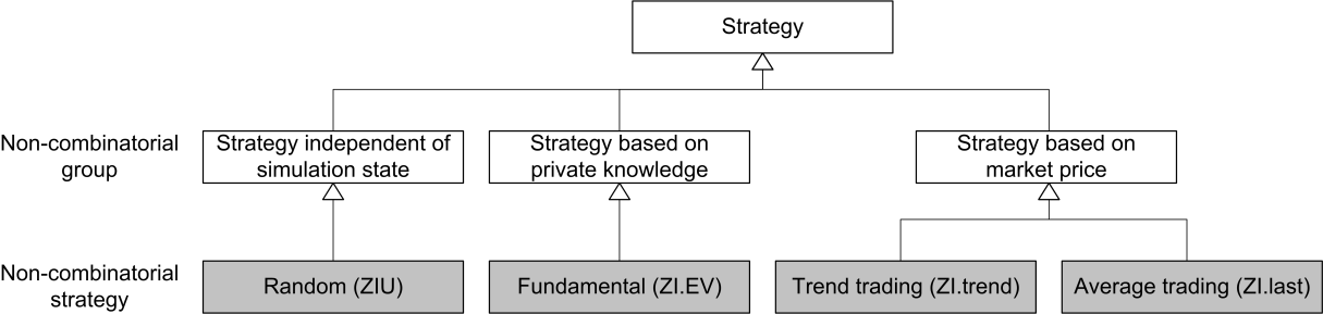
(3.1) Next, strategies are initially chosen out of the set of possible strategies in each of the three strategy groups which are non-combinatorial. They are kept as simple as possible to follow the idea of ZI-agents.
Strategies that are independent of the state of the simulation can be described as random. The literature has introduced zero intelligence unconstraint traders (Gode & Sunder 1993, p. 123), which sell and buy at any possible value determined by a uniform distribution. This strategy defines the validation baseline because it includes every action and is therefore minimally restrictive. In addition, random trading might pose a valid strategy for laboratory experiments and might even be meaningful in some cases (Fama 1965, p. 59). However, random trading seems to be the most basic strategy of the ZI strategy family. It is also supposed to be less successful in most environments compared to other zero intelligence strategies.
Strategies using the state of the agent are categorized as fundamental trading in the literature (e.g., Alfarano, Lux, & Wagner 2005, p. 21; Farmer & Joshi 2002, p. 150). In our simulation, a simple strategy is an adaptation of ZIC traders, i.e. zero intelligence expected value traders (ZI.EV) selling above and buying below the expected value[32]. The adaptation of ZIC is necessary because the true ZIC traders can only either buy or sell (Gode & Sunder 1993, p. 122). The expected value is calculated as the sum of all possible payoffs per states weighted with the probability known to the actors[33].
Validation hypothesis 1: The actions of trader xn | n ∈{1;…; 48} are best represented by ZI.EV strategy.
Strategies using the state of the market can be further broken down into (a) strategies trying to extrapolate past states and (b) strategies basing predictions on previous prices. (a) The former is described as trend trading (e.g., Farmer & Joshi 2002, p. 150) or herd trading (e.g., Alfarano et al. 2005, p. 22). The simplest strategy is a zero intelligence trend (ZI.trend) strategy buying below and selling above the trend price. It arrives at the trend price by extrapolating the last two prices and results in a predicted trend value that is the last price plus the difference between the last two prices[34].
Validation hypothesis 2: The actions of trader xn | n ∈{1;…; 48} are best represented by ZI.trend strategy.
(b) Finally, a strategy based on the market price is derived. An example can be found in literature like trading based on the last price(s). Duffy and Ünver (2006) develop a strategy that contains such a component (beside a fundamental trading component). The simplest strategy would be a zero intelligence last value (ZI.last) strategy which buys below and sells above the last price. This strategy is also consistent with random walk theory (Fama 1965, p. 56), according to which the best prediction of the next price is the last price. Therefore, an actor might consider trading on the last price as a strategy[35].
Validation hypothesis 3: The actions of trader xn | n ∈{1;…; 48} are best represented by ZI.last strategy.
(3.2) Next, the actors are assigned to the predefined classes in three steps. First, every action of each agent can be classified as compliant with a certain strategy or not compliant[36]. For instance, if a trader is selling for a price of 20 monetary units and the actor’s expected value is 30, the action is not compliant with the ZI.EV strategy. However, it might be compliant with other strategies. Unlike other empirical data, laboratory data allow for this classification, because the information of the actors is controlled by the experimenter. Second, the actor is classified into the strategy with which most of the actor’s actions conform. Third, the classification is tested against the null hypothesis. If the null hypothesis can be rejected, it remains in this class. Otherwise, it is re-classified into the class linked to the validation null hypothesis.
The validation null hypothesis of the classification is the ZIU strategy and leads to completely random actions by agents. The ZIU agents can sell and buy within a range from 0 to 100. Such an agent has an average compliance rate of about 49.5% with each rule[37]. On this basis, the validation hypotheses are tested against the validation null hypothesis.
Validation null hypothesis: The actions of trader xn | n ∈{1;…; 48} are best represented by ZIU strategy.
The 48 actors in the experiment of Hanson et al. (2006) are assigned to the 4 pure strategies documented in Table 9[38]. With 31-32 traders the majority is classified as ZI.EV traders; only 2-3 actors belong to ZI.trend or ZI.last. The validation baseline is not rejected against any of the validation hypotheses in 14 cases. Low correlation coefficients for the strategy compliance underline the diversity of the non-combinatorial strategies[39]. Furthermore, it has to be noted that the traders classified to the ZIU strategy are not necessarily trading randomly. In the case of a significance level of <.2, only 3 traders would not have been classified into to the classes ZI.EV, ZI.trend or ZI.last. These results lead to using the ZI.EV strategy as the default model for the agents in our simulation. In addition, ZIU will serve as a benchmark model. The other two strategies are not used, but subsequently combined with the ZI.EV strategy for the combinatorial strategies.
| Strategy group | Representative strategies | Valid. class | Number of actors assigned |
| Random | ZIU (random) | Null (Sig. <.05) | 14 |
| State of the agent | ZI.EV (expected value) | Class 1 | 31-32 |
| State of the market | ZI.trend (trend value) | Class 2 | 1-2 |
| ZI.last (last price) | Class 3 | 1 |
(4.1) Combinatorial strategies are derived next. ZI.EV serves as a starting point and is then combined with ZI.trend by calculating the average of the expected value and the trend value. Additionally, ZI.EV is also combined with ZI.last by calculating the average of the expected value and the last value. The combination of ZI.EV and ZI.trend is called ZI.EV.trend. The combinatorial strategy based on ZI.EV and ZI.last describes an instance of a trader type invented by Duffy and Ünver (2006) and is called near zero intelligence (N-ZI) traders. Combinatorial strategies as well as ZI.EV and ZIU are considered in the second validation as shown in Figure 6.
Validation hypothesis 4: The actions of trader xn | n ∈{1;…; 48} are best represented by ZI.EV.trend strategy.
Validation hypothesis 5: The actions of trader xn | n ∈ {1;…; 48} are best represented by N-ZI strategy.
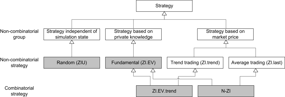
(4.2) The 48 actors are then assigned to the 2 revised classes as well as the 2 standard classes (ZIU and ZI.EV) as documented in Table 10. Approximately the same number of traders is classified into ZI.EV and N-ZI respectively. No actor can uniquely be classified into ZI.EV.trend and there are only two less ZIU traders for the combinatorial than for the non-combinatorial strategies. The high correlation coefficients[40] expose the reduced diversity of the strategies. It is caused by the component shared by all strategies in Table 10 – the expected value. These results lead to including the N-ZI strategy to the set of strategies used in our simulation.
| Strategy group | Representative strategies | Valid. class | Result |
| Random | ZIU (fully random) | Null (Sig. <.05) | 12 |
| Fundamental | ZI.EV (expected value) | Class 1 | 13-21 |
| Fundamental + trend | ZI.EV.trend (0.5*exp. v.+0.5*t. v.) | Class 4 | 0-7 |
| Fundamental + average | N-ZI (0.5*exp.v.+0.5*last price) | Class 5 | 12-22 |
Overall, resulting from our micro validation homogenous and heterogeneous models are selected. First, two homogenous models, i.e., models where all traders are following the same strategy, are suggested (ZI.EV, N-ZI) following the micro validation. Finally, heterogeneous models containing agents with different strategies are added. Mix 1 considers the equal division of the actors and is restricted by a balanced information distribution to outweigh the ZI.EV strategy. It comprises the two strategies derived from the validation without the ZIU strategy. Therefore, the heterogeneous model Mix 1 can be seen as a “lower boundary” of random traders. The heterogeneous model Mix 2 contains the two strategies derived from the validation and the ZIU strategy given that the ZIU strategy could not be rejected for 12 actors in the combinatorial case. Therefore, it represents the idea of an “upper border” of random traders.
Notes
- The terms “information markets”, “decision markets”, “electronic markets”, “virtual markets”, “political stock markets”, “election stock markets”, “artificial markets” and “idea futures” can found in the literature as well (Tziralis & Tatsiopoulos 2007, pp. 76-77).
- This work is a revised and substantially extended version of (Klingert & Meyer 2012b) presented at ECMS 2012 in Koblenz and elaborates on the PhD thesis of one of the authors (Klingert 2013). It provides additionally to the ECMS contribution an extensive description of the micro validation and investigates further hypotheses. Beyond, further feedback is considered, among others of the participants at ECMS 2012.
- The reason why companies set up such markets is that concerning the information they want to generate typically no usable market exists. This is also often the case for prediction markets used in other contexts. Still, often the ability of markets to aggregate dispersed information described by Hayek can sometimes be used by looking at already existing (future) markets (for examples see Surowiecki 2010). E.g., the expected outcome of elections and possible changes in this respect might also be reflected in the stock market of a country. A practical challenge of prediction markets is possible susceptibility to manipulation (Hansen, Schmidt, & Strobel 2004; Hanson, Oprea, & Porter 2006).
- A notable exception in this respect is the work by Brahma et al. (2012).
- The talk by Ledyard is not published, but as empirical insight regarding the difference of CDA and LMSR is rare, we cite here the paper in which his talk is mentioned.
- Even the number for the average prediction market in a corporate context is higher despite the fact that it generally involves fewer traders than other prediction markets.
- The variance of the price from the correct value is used as a measure for the accuracy level (Hanson et al. 2006, p. 456). Another related criterion is the time a mechanism needs to incorporate new information. This is not in the focus of this paper. Concerning this and related issues the paper by Brahma et al. (2012) can be seen as a very useful complementary contribution comparing an refined version of the LMSR and their Bayesian Market Maker. See also the next endnote for the other metrics used in their paper.
- Brahma et al. (2012) use different metrics due to the different simulation targets and the resulting research questions, which are partially overlapping. Both papers measure the accuracy of the prediction market and therefore employ very similar measures (we follow Hanson et al. 2006 and measure accuracy as the variance between the price and the correct value, Brahma et al. 2012 use the RMSD which is the root mean square deviation). Both papers also address the reliability of the market towards the end of trading. We use the standard deviation of the last prices, while Brahma et al. (2012) look at RMSDeq. This difference is again driven by the different foci of research. We want to assess the risk of making wrong decisions based on “extreme” predictions. Brahma et al. (2012) uses the RMSDeq to address a specific shortcoming of the LMSR, i.e. that it tends to fluctuate even after reaching the true value. This property of the LMSR is not in the focus of our research, as the CDA is known to be much more volatile than the LMSR. We measure the number of trades, as this gives an indication for the liquidity in the market and its related ability to aggregate information. Brahma et al. (2012) measure the bid-ask-spread. This gives also an indication for the liquidity in the market, as a higher spread also implies a lower liquidity. At the same time the authors consider this as a measure for the convergence of the respective market maker’s beliefs. Given our differing research focus, adding these metrics would not add enough value compared to the cost of increasing the complexity of this paper. For a discussion of their results related to the ones of our paper see (Section 5).
- The program code and explanations concerning it will be provided by the authors upon request.
- The knowledge distribution chosen by Hanson et al. (2006) is partially certain and might appear rather specific. Nevertheless, there are circumstances where similar information distributions could exist in reality. Let us think about an IT-consulting company predicting its revenue figures with a corporate prediction market. Maybe a division of this company is mainly dependent on two projects: A Blueprint project with a volume of 40 Mio. Euros and a dependent realization project with a volume of 60 Mio. Euros. The possible outcomes in this case would be 0 Euros, if no project will be executed, 40 Mio. Euros if the first one is executed and 100 Mio. Euros if both projects are executed. In this case, an employee might have certain knowledge about an approved Blueprint project which will be executed for sure without knowing more details about the second project.
- It is assumed that the actors in the laboratory experiment have comparable reaction times.
- This is an important difference to other studies also referring to experiments. For example, the focus of Hommes (2011) is to combine experiments and simulation to show that their models can be fitted to their experimental data and helps to explain some observed stylized facts. Still, there are also other studies which try to go beyond the original settings (see Bravo, Squazzoni, & Boero 2012). A crucial issue when doing so is to consider whether the behavioral strategies derived from the original laboratory setting still hold for the new settings derived.
- The parameter \(b\) bounds the loss of the market maker, but also influences how adaptive the market maker is and the liquidity in the market. Such a market maker who is very adaptive results in large bid-ask spreads. This reduces the liquidity in the market (Brahma et al. 2012). Hence, a tradeoff exists limiting possible losses and sufficient liquidity. For mathematical details, see Brahma et al. (2012) and Pennock and Sami (2007).
- Beside the initial endowment of money, the CDA may have additional costs due to the initial endowment of stocks, if the correct value is 40 or 100. Then each stock pays the trader 40 or 100 monetary units. In LMSR, the traders do not receive an initial endowment of stocks and do not get this additional payoff. However, they receive an additional payoff by the loss of the market maker. The b-value regulates this loss. When choosing a level for b a tradeoff exists between not allowing too much possible loss (which should be in our setting comparable to the costs of the CDA) and a liquid market with low fluctuations around the equilibrium (Brahma et al. 2012). Therefore, when setting the parameter b, we have experimented with b and fixed it at a sufficiently high level. Consistent with these sensitivity analyses, we fixed the value for b as 17.31 in our experiments as a control variable.
- As zero intelligence traders are bounded by simple rules, they should not be considered as completely random. The only exception is the strategy ZIU.
- The micro level refers to the actions of the agents in the simulation and the actors in the laboratory experiment, for example.
- To the knowledge of the authors, they have not been statistically validated in subsequent papers either. This is not very surprising because zero intelligence agents were originally not designed to represent human behavior. They have been designed to show that even very simple strategies at the micro level can result in patterns typically observed at markets at the macro level.
- Brahma et al. (2012, pp. 230-231) also investigate the effects of different trading strategies in their comparative analysis. They distinguish also between several types of technical and fundamental traders, but do not provide an empirical validation of the trading strategies. Hommes (2011) provides an interesting example of empirically validated behavior in asset markets, making a claim for the heterogeneous expectation hypothesis. In some of the settings, he also includes fundamental traders, but overall he suggests a behavioral model that is able to switch between different forecasting heuristics. It should be mentioned that in his settings agents only forecast prices and do not buy stocks and that his study has a different scope.
- The problem of overfitting simulation models to historical data has already been discussed in the literature (Law 2014).
- Each strategy should be represented by an even number because the agents can have two different knowledge components, i.e. one agent has an expected value above and one below the true value. An even number of agents ensures an appropriate separation between knowledge and strategy to analyze the interaction effect. Two more restrictions have to be taken into account. Only a natural number of agents is possible and the distribution should be valid for 6 agents because the experimental design starts with 12 agents and tries to test a linear relationship of 6, 12 and 18 agents in a 3k-design of experiment.
- Average accuracy level: Empirical (1185), ZI.EV (1079), N-ZI (1030), Mix 1 (1084), Mix 2 (1772), ZIP (1420), ZIU (2558).
- For example, CV 0 means, that 50 % (50 %) of the agents know, that the correct value is not 40 (100).
- Simulating the default setting 10,000 times, the variance increasingly stabilizes (see Lorscheid et al. 2012,p. 51-52). Due to computing time restrictions and a clear decrease of instability after the first runs, 100 runs per factor combination are performed. The high significance levels of our statistical analyses indicate that the simulation model behavior is sufficiently stable.
- \(Partial\, \eta^2= \frac{SS_{treatment}}{(SS_{treatment}+ SS_{error})}\) (Pierce, Block, & Aguinis 2004).
- The average amount of trades based on the ZIP strategy in the default setting is 26.86 (CDA) and 38.08 (LMSR) respectively. Over all settings the difference is even smaller with an average of 29.67 (CDA) and 30.14 (LMSR).
- Brahma et al. (2012, p. 231) also investigated the effects of trading strategies and their results supported their relevance too. The overall trend in their simulation experiments is that with more fundamental traders the accuracy gets better (which makes sense as the noise in the market is reduced).
- The maximum deviation of the median is only 2.18 monetary units.
- Each strategy should be represented by an even number because the agents can have two different knowledge components, i.e. one agent has an expected value above and one below the true value. An even number of agents ensures an appropriate separation between knowledge and strategy to analyze the interaction effect. Two more restrictions have to be taken into account. Only a natural number of agents is possible and the distribution should be valid for 6 agents because the experimental design starts with 12 agents and tries to test a linear relationship of 6, 12 and 18 agents in a 3k-design of experiment.
- Beyond, we checked several other settings not described here. For example, the simulation is relatively stable concerning its main results with a higher number of agents not simulated in our experiments (e.g., 50 or 100 number of agents) comparing CDA and LMSR in the standard setting.
- The term ZI agents stems from the fact that the rules constraining an agent’s budget were not set by the agent but by the market in the original paper (Gode & Sunder 1993). The agent behaves randomly within this constraint.
- Strategy: State of the simulation [x Random] → Action (Wooldridge 2002, p. 31-42)
- This strategy follows the spirit of ZI-agents. For example, the component of N-ZI traders (Duffy & Ünver 2006) which represents fundamental trading is similar to the ZI.EV traders.
- \(\text{Expected value} = \sum^{\text{Number of states}}_{s=1}\text{payoff}_s*\text{probability}_s\).
- Trend value = pricet + (pricet - pricet-1).
- Last value = pricet.
- Note: Accepting an ask for a price of x is considered as buying at a price of x. Accepting a bid for a price of x is considered as selling at a price of x.
- Note: Accepting an ask for a price of x is considered as buying at a price of x. Accepting a bid for a price of x is considered as selling at a price of x.
- The agents in the four experiments with replication treatment arenot analyzed separately in order toreduce the complexity of the validation. Separating the experiments, the ZI.EV strategy is still the dominant strategy with at least 7 actors in the ZI.EV class in each of the 4 experiments.
- Comparing the percentage of compliant actions for two strategies, Pearson’s correlation coefficient is 0.13 (ZI.EV vs. ZI.trend), 0.25 (ZI.EV vs. ZI.last) and -0.19 (ZI.trend vs. ZI.last) (none of the correlations reaches a p-level of .05).
- Comparing the percentage of compliant actions for two strategies yields a Pearson’s correlation coefficient of 0.92*** (ZI.EV vs. ZI.EV.trend), 0.90*** (ZI.EV vs. N-ZI) and 0.88*** respectively (ZI.EV.trend vs. N-ZI) (for all correlations: *** p < .001).
References
ALFARANO, S., Lux, T., & Wagner, F. (2005). Estimation of Agent-Based Models: The Case of an Asymmetric Herding Model. Computational Economics, 26(1), 19-49. [doi:10.1007/s10614-005-6415-1 ]
ANTWEILER, W. (2013). Liquidity Provision and Cross Arbitrage in Continuous Double-Auction Prediction Markets. Journal of Prediction Markets, 7(3), 61-86.
ATANASOV, P., Rescober, P., Stone, E., Swift, S. A., Servan-Schreiber, E., Tetlock, P., Ungar, L., & Mellers, B. (2016). Distilling the Wisdom of Crowds: Prediction Markets Vs. Prediction Polls. Management Science, 63(3), 691-706. [doi:10.1287/mnsc.2015.2374 ]
BOERO, R., & Squazzoni, F. (2005). Does Empirical Embeddedness Matter? Methodological Issues on Agent-Based Models for Analytical Social Science. Journal of Artificial Societies and Social Simulation, 8(4), 6: https://www.jasss.org/8/4/6.html.
BRAHMA, A., Chakraborty, M., Das, S., Lavoie, A., & Magdon-Ismail, M. (2012). A Bayesian Market Maker. Paper presented at the Proceedings of the 13th ACM Conference on Electronic Commerce. [doi:10.1145/2229012.2229031 ]
BRAVO, G., Squazzoni, F., & Boero, R. (2012). Trust and Partner Selection in Social Networks: An Experimentally Grounded Model. Social Networks, 34(4), 481-492. [doi:10.1016/j.socnet.2012.03.00 ]
BRAY, D., Croxson, K., & Dutton, W. (2008). Information Markets: Feasibility and Performance. Oxford Internet Institute DPSN Working Paper Series No. 10. Working paper. Oxford Internet Institute. [doi:10.2139/ssrn.1302896 ]
CAMERER, C. F., Dreber, A., Forsell, E., Ho, T.-H., Huber, J., Johannesson, M., Kirchler, M., Almenberg, J., Altmejd, A., & Chan, T. (2016). Evaluating Replicability of Laboratory Experiments in Economics. Science, 351(6280), 1433-1436.
CHEN, K.-Y., & Plott, C. (2002). Information Aggregation Mechanisms: Concept, Design and Implementation for a Sales Forecasting Problem. Working paper. Social Science Working Paper 1131. California Institute of Technology, Pasadena. [doi:10.1920/wp.cem.2002.0202 ]
CHEN, S. H. (2012). Varieties of Agents in Agent-Based Computational Economics: A Historical and an Interdisciplinary Perspective. Journal of Economic Dynamics & Control, 36(1), 1-25.
CHEN, Y., & Pennock, D. M. (2010). Designing Markets for Prediction. AI Magazine, 31(4), 42-52. [doi:10.1609/aimag.v31i4.2313 ]
CLIFF, D., & Bruten, J. (1997). More Than Zero Intelligence Needed for Continuous Double-Auction Trading HP Technical Report. Bristol: HP Laboratories.
COWGILL, B., & Zitzewitz, E. (2015). Corporate Prediction Markets: Evidence from Google, Ford, and Firm X. The Review of Economic Studies, 82(4), 1309-1341. [doi:10.1093/restud/rdv014 ]
DREBER, A., Pfeiffer, T., Almenberg, J., Isaksson, S., Wilson, B., Chen, Y., Nosek, B. A., & Johannesson, M. (2015). Using Prediction Markets to Estimate the Reproducibility of Scientific Research. Proceedings of the National Academy of Sciences, 112(50), 15343-15347.
DUFFY, J., & Ünver, M. U. (2006). Asset Price Bubbles and Crashes with near-Zero-Intelligence Traders. Economic Theory, 27(3), 537-563. [doi:10.1007/s00199-004-0570-9 ]
FAMA, E. F. (1965). Random Walks in Stock Market Prices. Financial Analysts Journal, 21(5), 55-59.
FARMER, J. D., & Joshi, S. (2002). The Price Dynamics of Common Trading Strategies. Journal of Economic Behavior & Organization, 49(2), 149-171. [doi:10.1016/S0167-2681(02)00065-3 ]
FORSYTHE, R., Forrest, N., George, R. N., & Jack, W. (1992). Anatomy of an Experimental Political Stock Market. American Economic Review, 82(5), 1142-1161.
GILBERT, N., & Troitzsch, K. G. (2005). Simulation for the Social Scientist (2nd ed.). Maidenhead: Open University Press.
GODE, D. K., & Sunder, S. (1993). Allocative Efficiency of Markets with Zero-Intelligence Traders: Market as a Partial Substitute for Individual Rationality. Journal of Political Economy, 101(1), 119-137.
GRIMM, V., Berger, U., Deangelis, D. L., Polhill, J. G., Giske, J., & Railsback, S. F. (2010). The Odd Protocol for Describing Individual-Based and Agent-Based Models: A First Update. Ecological Modelling, 221(23), 2760-2768. [doi:10.1016/j.ecolmodel.2010.08.019 ]
GRIMM, V., Revilla, E., Berger, U., Jeltsch, F., Mooij, W. M., Railsback, S. F., Thulke, H. H., Weiner, J., Wiegand, T., & Deangelis, D. L. (2005). Pattern-Oriented Modeling of Agent-Based Complex Systems: Lessons from Ecology. Science, 310(5750), 987-991.
HANSEN, J., Schmidt, C., & Strobel, M. (2004). Manipulation in Political Stock Markets: Preconditions and Evidence. Applied Economics Letters, 11(7), 459-463. [doi:10.1080/1350485042000191700 ]
HANSON, R. (2003). Combinatorial Information Market Design. Information Systems Frontiers, 5(1), 107-119.
HANSON, R. (2009). On Market Maker Functions. Journal of Prediction Markets, 3(1), 61-63.
HANSON, R., Oprea, R., & Porter, D. (2006). Information Aggregation and Manipulation in an Experimental Market. Journal of Economic Behavior & Organization, 60(4), 449-459.
HEALY, P. J., Linardi, S., Lowery, J. R., & Ledyard, J. O. (2010). Prediction Markets: Alternative Mechanisms for Complex Environments with Few Traders. Management Science, 56(11), 1977-1996. [doi:10.1287/mnsc.1100.1226 ]
HEATH, B., Hill, R., & Ciarallo, F. (2009). A Survey of Agent-Based Modeling Practices (January 1998 to July 2008). Journal of Artificial Societies and Social Simulation, 12(4), 9: https://www.jasss.org/12/4/9.html.
HEINE, B.-O., Meyer, M., & Strangfeld, O. (2005). Stylised Facts and the Contribution of Simulation to the Economic Analysis of Budgeting. Journal of Artificial Societies and Social Simulation, 8(4), 4: https://www.jasss.org/8/4/4.html.
HOMMES, C. (2011). The Heterogeneous Expectations Hypothesis: Some Evidence from the Lab. Journal of Economic Dynamics and Control, 35(1), 1-24.
HORN, C. F., Ivens, B. S., Ohneberg, M., & Brem, A. (2014). Prediction Markets: A Literature Review 2014. The Journal of Prediction Markets, 8(2), 89-126.
IVANOV, A. (2008). Electronic Prediction Markets. Analyx Reference Information. Poznan.
JIAN, L., & Sami, R. (2012). Aggregation and Manipulation in Prediction Markets: Effects of Trading Mechanism and Information Distribution. Management Science, 58(1), 123-140. [doi:10.1287/mnsc.1110.1404 ]
KANTARDZIC, M. (2003). Data Mining: Concepts, Models, Methods and Algorithms. Hoboken: Wiley.
KLEIJNEN, J. P. C. (2015). Design and Analysis of Simulation Experiments (Vol. Second Edition). Switzerland: Springer International Publishing.
KLINGERT, F. M. A., & Meyer, M. (2012a). Effectively Combining Experimental Economics and Multi-Agent Simulation: Suggestions for a Procedural Integration with an Example from Prediction Markets Research. Computational & Mathematical Organization Theory, 18(1), 63-90.
KLINGERT, F. M. A., & Meyer, M. (2012b). 'Comparing prediction market mechanisms using an experiment-based multi-agent simulation.' In Klaus G. Troitzsch, Michael Möhring, und Ulf Lotzmann (eds.), Proceedings of the European Conference on Modelling and Simulation, 654-661, Koblenz. [doi:10.7148/2012-0654-0661 ]
KLINGERT, F. M. A. (2013). Corporate prediction markets: a multi-agent simulation based on laboratory experiments. Dissertation TU Hamburg-Harburg.
KLINGERT, F. M. A. (2017). The Structure of Prediction Market Research: Important Publications and Research Clusters. The Journal of Prediction Markets, 11(1), 51-65.
LAW, A. M. (2014). Simulation Modeling and Analysis (Vol. 5th International Edition). New York, New York: McGraw-Hill, Inc.
LEDYARD, J., Hanson, R., & Ishikida, T. (2009). An Experimental Test of Combinatorial Information Markets. Journal of Economic Behavior & Organization, 69(2), 182-189. [doi:10.1016/j.jebo.2008.04.010 ]
LORSCHEID, I., Heine, B.-O., & Meyer, M. (2012). Opening the ‘Black Box’of Simulations: Increased Transparency and Effective Communication through the Systematic Design of Experiments. Computational and Mathematical Organization Theory, 18(1), 22-62.
OPREA, R., Porter, D., Hibbert, C., Hanson, R., & Tila, D. (2007). Can Manipulators Mislead Market Observers? Working Paper. Working Paper. University of California. Santa Cruz.
OTHMAN, A. (2008). Zero-Intelligence Agents in Prediction Markets. Paper presented at the 7th international joint conference on Autonomous agents and multiagent systems, Estoril: http://portal.acm.org/citation.cfm?id=1402346#.
OTHMAN, A., & Sandholm, T. (2010a). Automated Market-Making in the Large: The Gates Hillman Prediction Market. Paper presented at the Conference on Electronic Commerce, Cambridge, MA. [doi:10.1145/1807342.1807401 ]
OTHMAN, A., & Sandholm, T. (2010b). When Do Markets with Simple Agents Fail? Paper presented at the International Conference on Autonomous Agents and Multiagent Systems, Toronto.
PENNOCK, D. M., & Sami, R. (2007). Computational Aspects of Prediction Markets. In N. Nisan, T. Roughgarden, E. Tardos & V. V. Vazirani (Eds.), Algorithmic Game Theory (pp. 651-674). [doi:10.1017/CBO9780511800481.028 ]
PIERCE, C. A., Block, R. A., & Aguinis, H. (2004). Cautionary Note on Reporting Eta-Squared Values from Multifactor Anova Designs. Educational and psychological measurement, 64(6), 916-924.
ROTH, A. E. (2008). What Have We Learned from Market Design? The Economic Journal, 118(527), 285-310. [doi:10.1111/j.1468-0297.2007.02121.x ]
ROTHSCHILD, D. M., & Sethi, R. (2016). Trading Strategies and Market Microstructure: Evidence from a Prediction Market. Journal of Prediction Markets, 10(1), 1-29.
SECCHI, D., & Seri, R. (2016). Controlling for False Negatives in Agent-Based Models: A Review of Power Analysis in Organizational Research. Computational and Mathematical Organization Theory, 22(1), 1-28.
SLAMKA, C., Skiera, B., & Spann, M. (2013). Prediction Market Performance and Market Liquidity: A Comparison of Automated Market Makers. IEEE Transactions on Engineering Management, 60(1), 169-185.
SMITH, V. L. (1962). An Experimental Study of Competitive Market Behavior. The Journal of Political Economy, 70(2), 111-137. [doi:10.1086/258609 ]
SPANN, M., & Skiera, B. (2003). Internet-Based Virtual Stock Markets for Business Forecasting. Management Science, 49(10), 1310-1326.
SUROWIECKI, J. (2010). The Wisdom of Crowds: Why the Many Are Smarter Than the Few. London: Abacus.
TROITZSCH, K. G. (2014). Simulation Experiments and Significance Tests. In S. Leitner & F. Wall (Eds.), Artificial Economics and Self Organization (pp. 17-28). Switzerland Springer.
TSENG, J. J., Li, S. P., Chen, S. H., & Wang, S. C. (2009). Emergence of Scale-Free Networks in Markets. Advances in Complex Systems, 12(1), 87-97. [doi:10.1142/S021952590900209X ]
TZIRALIS, G., & Tatsiopoulos, I. (2007). Prediction Markets: An Extended Literature Review. Journal of Prediction Markets, 1(1), 75-91.
WOLFERS, J., & Zitzewitz, E. (2004). Prediction Markets. Journal of Economic Perspectives, 18(2), 107-126. [doi:10.1257/0895330041371321 ]
WOOLDRIDGE, M. (2002). An Introduction to Multiagent Systems. Chichester: Wiley.