
| Erratum: The names, von Neumann and Moore, (neighborhoods) were interchanged in the first version of this article, published on 31 January 2018. Although this error did not affect the findings of the article, this version has been corrected. [Added on the author's request on 02 February 2018; the author and the editor thank Mr Thomas Feliciani, Groningen University, for spotting the error and informing us promptly] |
Introduction
Background on modeling inequalities and classes and the use of dynamics on lattices
The question of inequalities and classes has received a lot of attention from social scientists and modelers. Early influential precursors were Wilfried Pareto with the wealth distribution curve (1986) and Thomas Schelling with the study of segregation (1971, 2006).
The framework of multi–agents iterated games is often used. In the tribute game, one agent requests tribute, and the other agent either pays the tribute or has to fight. The chances to win the fight depends upon the relative strength of the agents, a quantity which is increased for the agent who wins the fight and receives the tribute; it is decreased for the other agent. Axelrod (1997b); Bonabeau et al. (1995) have shown that when iterated, the tribute game results in the dominance of some agents over others.
In the bargaining game introduced by Nash Jr (1950), agents have to share a pie. They independently fix the fraction of the pie that they demand. If the sum of their demands is less than the size of the pie, their demands are satisfied. Otherwise, they get nothing. When the game is iterated among a society of agents, Axtell et al. (2001), Bowles & Naidu (2006) and Weisbuch (2018) have shown that different outcomes can be obtained. Societies can be either egalitarian or structured in classes. In their paper entitled “Emergence of Classes in a Multi–Agent Bargaining Model", Axtell et al. (2001) highlight the role of a priori neutral tags in favouring the emergence of classes. Poza et al. (2011) and Santos et al. (2012) proposed extensions of their model to respectively lattice interactions and small world networks.
Another approach to the dynamics of Nash bargaining game was proposed by Skyrms (2014) who calls the game “Divide The Cake". Skyrms (2014) uses replicator dynamics based up biological evolution metaphor: Agent learning is replaced by a selection process according to which the most successful agents replicate faster.
Weisbuch (2018) revisited Axtell et al. (2001) using more elaborate memorisation and decision models. His version to be further called BOMA (for Boltzmann Moving Average) has shown that the outcome of the iterated bargaining game is strongly constrained by the initial conditions: he then interpreted this result as demonstrating the persistence of inequity rather than the emergence of classes.
The purpose of the present paper is to study the dynamics of Weisbuch (2018) version of the iterated bargaining game on a lattice. Many game theoretic models display new properties when played on a lattice. The best known example is the imitation game called in its binary version the voters model. Agents on a lattice take the majority opinion among their neighbours’ opinions. Rather than the uniform yes or no opinion obtained when agents follow the majority of all other agents, dynamics on lattice results in the segregation of opinions in uniform domains in the lattice as discussed in the review of Castellano et al. (2009). Epstein (2006) has shown that when agents play the prisoner’s dilemma game on a lattice domains of cooperation can emerge which is never the case in the absence of a social network. Following the above two references, we might expect domain formation and possibly new dynamical properties or new conditions for the emergence of significant behaviours by running simulations on a lattice.
We start with a very brief exposition of the papers of Axtell et al. (2001) and Poza et al. (2011). We then introduce the BOMA model of Weisbuch (2018) and give the main results obtained in a fully connected network, i.e. when any agent can play with any other agent. Section 2 describes the application of the BOMA model to the lattice topology. Various spatio–temporal patterns are observed depending upon parameters and initial conditions. These dynamical regimes are interpreted in terms of social norms, such as equity or inequity. We further report the transitions among dynamical regimes according to changes in parameters. The influence of arbitrary tags introduced by Axtell et al. (2001) is discussed in Section 3. Section 4 summarises possible interpretations in social and political sciences. Appendix A provides further details about dynamics in the transition neighborhood. Appendix B provides programming details.
The original model of Axtell, Epstein and Young
Let us briefly recall the original hypotheses and the main results of Axtell, Epstein and Young (Axtell et al. 2001).
- Framework: pairs of agents play a bargaining game introduced by Nash Jr (1950) and Young (1993). During sessions of the game, each agent can, independently of his opponent, request one among three demands: L(ow) demand 30 perc. of a pie, M(edium) 50 perc. and H(igh) 70 perc. As a result, the two agents get at the end of the session what they demanded when the sum of both demands is less or equal to 100 perc.; otherwise they don’t get anything. The corresponding payoff matrix is written in Table 1. At each step, a random pair of agents is selected to play the bargaining game. The iterated game is played for a large number of sessions, much larger that the total number of agents which can then learn from their experience how to improve their performance.
- Learning and memory: Agents keep records of the previous demands of their opponents, e.g. for 10 previous moves.
- Choosing the next move: at each iteration step, pairs of agent are randomly selected to play the bargaining game. They most often choose the move that optimises their expected payoff using the memory of previous encounters as a surrogate for the actual probability distribution of their opponent’s next moves. With a small probability \(\epsilon\), e.g. 0.1, they choose randomly among L, M, H.
The main results obtained by Axtell et al. (2001) from numerical simulations are:
- They observe different transient configurations which they interpret as “norms", e.g. the equity norm is observed when all agents play M.
- Their most fascinating result is obtained when agents are divided into two populations with arbitrary tags, e.g. one red and one blue. When agents take into account tags for playing and memorising games (in other words when agents play separately two games, one intra–game against agents with the same tag and another inter–game against agents with a different tag), one observes configurations in the inter– game such that one population always play H while the other population plays L; they interpret such inequity norm as the emergence of classes, the H playing population being the upper class.
Equivalent results are obtained when agents are connected via a social network as observed by Poza et al. (2011) on a square lattice and Santos et al. (2012) on a small world network as opposed to the full connection structure used by Axtell et al. (2001).
| L | M | H | |
| L | 0.3 | 0.3 | 0.3 |
| M | 0.5 | 0.5 | 0 |
| H | 0.7 | 0 | 0 |
The Moving Average–Boltzmann choice cognitive model
Weisbuch (2018) starts from the same bargaining game as Axtell et al. (2001) with a payoff matrix written in Table 1, but uses different coding of past experience (moving average of past profits) and choice function (Boltzman function), hence the acronym BOMA for the model.
The model is derived from standard models of reinforcement learning in cognitive science, see for instance Weisbuch et al. (2000).
Rather than memorising a full sequence of previous games as in Axtell et al. (2001), agents learn and code their memories as three “preference coefficients" \(J_j\) for each possible move \(j\), based on a moving average of the profits they made in the past when playing \(j\). \(J_1\) is the preference coefficient for playing \(H\), \(J_2\) for \(M\) and \(J_3\) for \(L\). Following time interval \(\tau\) after a transaction \(J_j\) are updated according to:
| $$J_{j}(t+\tau) = (1-\gamma) \cdot J_{j}(t) + \; \pi_{j}(t), \qquad \forall j,$$ | (1) |
These preference coefficients are then used to choose the next move in the bargaining game. Agents face an exploitation/exploration dilemma: they can decide to exploit the information they earlier gathered by choosing the move with the highest preference coefficient or they can check possible evolutions of profits by randomly trying other moves. Rather than using a constant rate of random exploration \(\epsilon\) as in Axtell et al. (2001), the probability of choosing demand \(j\) is based on the Boltzmann choice, also called logit function (Anderson et al. 1992):
| $$P_{j} = \frac{\exp (\beta J_{j})}{\sum_{j}{\exp (\beta J_{j})}} , \qquad \forall j,$$ | (2) |
Comparing our model with the one proposed by Axtell et al. (2001):
- The moving average is an efficient coding of past experiences through connection coefficients \(\bf{J}\) as proposed in cognitive science by Rumelhart et al. (1987), Hopfield (1982) and Ackley et al. (1985). It corresponds to a gradual rather than abrupt decrease of previous memories, it is based on agent’s own experience in terms of profit rather than the observation of her opponents’ moves and it uses less memory. The coding of agent’s memory by a vector rather than the use of a sequence of 3 x memory size matrix used by Axtell et al. (2001) allows to conveniently relate the observed dynamics to initial conditions which would be quite difficult with the matrix coding.
- Boltzman choice has a random character as the constant probability noise introduced in Axtell et al. (2001), but furthermore the choice depends upon the differences in experienced profits; we might expect agents to be less hesitant when their previous experience resulted in very different preference coefficients.
Main results of the Moving Average–Boltzmann choice model for the well mixed case
These are the main results of the Moving Average–Boltzmann choice model for the well mixed case:
- A single reduced parameter \(\beta/\gamma\) governs the dynamics[1].
- A disordered state is observed such as agents do not have fixed preferences when \(\beta/\gamma \le 4\).
- When \(\beta/\gamma \ge 4\) the dynamics evolve towards well characterized attractors such that agents have strong preferences: a “fair" attractor such that all agents play M, a “timid" attractor such that all play L and an “unfair" or “inequity" attractor such that some play H while others play L. Which attractor is reached depends upon the unique reduced parameter \(\beta/\gamma\) and upon initial conditions characterised by the initial distribution of preference coefficients.
- When tags are introduced, agents might play M when opposed to agents with the same tag, while they play H against agents with a different tag, who play themselves systematically L, a condition called “discriminatory norm" by Axtell et al. (2001). However, the occurrence of this asymmetric attractor depends upon initial conditions which should already be biased towards such an asymmetry. Weisbuch (2018) then interpreted this effect as a “persistence of discrimination" rather than “emergence of classes" as Axtell et al. (2001) did.
The Moving Average–Boltzmann Model on Lattice
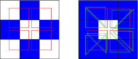
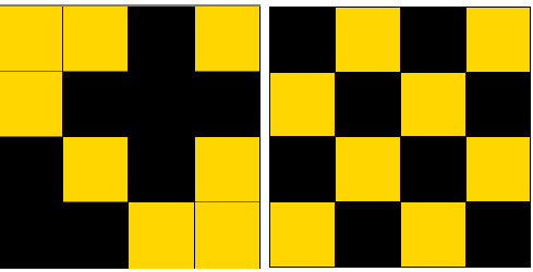
Each agent occupies a cell in a square lattice, one agent per cell. We used either von Neumann neighborhood, each agent interacting with 4 neighbors to be further called vN4 (Figure 5, left) or Moore neighborhood, each agent interacting with 8 neighbors to be further called M8 (Figure 5, right). The lattice boundaries are connected, top to bottom and left to right (periodic boundary conditions).
The initial conditions concern the \(\bf J\) coefficients which are randomly set according to uniform distributions. An initial condition noted \(hml\) means that \(J_1\) was randomly chosen between 0 and \(h\), \(J_2\) between 0 and \(m\) and \(J_3\) between 0 and \(l\). We used for instance initial conditions 444 and 414.
At each iteration step, a pair of neighboring agents is randomly chosen to play the bargaining game; they chose a move H, M or L according to the logit rule (Equation 2) and update their \(\bf J\) coefficients according to their profit (Equation 1). A new random pair is then selected to play the game and so on ... until some kind of stability is achieved. Since the choice process is probabilistic, stability here refers to the invariance of the distributions of \(J_j\) after large iteration times. Typical iteration times to check stability are 180 000 games per agent. A human agent playing one game per day during 80 years would only play 29 200 games.
Simulations on lattices display common properties with those observed in the well mixed topology.
- Different dynamics regimes are observed depending upon parameters values: disordered regimes at lower \(\beta/\gamma\) values and several ordered regimes at higher \(\beta/\gamma\) values. Regimes are separated by transitions.
- Agents have strong opinions about their choices for higher \(\beta/\gamma\) values: \(\bf J\)’s most often have only one non zero component which saturates at
where \(<\pi_i>\) is the average[1] payoff obtained by the agent.$$J_i = \frac{<\pi_i>}{\gamma}$$ (3)
The new feature displayed by lattice dynamics is the spatial arrangement of choices in patterns in the ordered phases.
The results are presented on figures 1, 2, 4, 9 etc. as snapshots of the lattice after long iteration times representing agents \(\bf J\) coefficients according to an rgb color code such that the r coefficient codes for \(J_1\), the g coefficient codes for \(J_3\)and the b coefficient codes for \(J_2\). For instance, a red cell indicate that the agent plays H, a blue cell M and a green cell L. Let us here recall two important conventions for the presentation of results:
- The initial conditions often determine the outcome of the dynamics: we use the hml notation where the figures are upper limits of the uniform distributions of preference coefficients.
- Rather than varying the two model parameters \(\beta\) and \(\gamma\), we only vary \(\beta\) with a fixed value of \(\gamma=0.1\) because the formal analysis of the mean field approximation in Weisbuch (2018) demonstrates the existence of a single reduced parameter \(\beta/\gamma\) which allows to rescale all results when \(\gamma \neq 0.1\). More precisely, the fraction of agents playing H, M or L and the positions of the transitions depend upon \(\beta/\gamma\) , while the magnitude of the preference coefficients \(J\) are inversely proportional to \(\gamma\)and the relaxation time towards equilibrium is proportional to \(\beta\). We checked the validity of this prediction during simulations; its limits are discussed in the appendix.
Patterns (see Figure 1)
Disordered regime
Let us start with the disordered regime observed at low \(\beta/\gamma\) values.
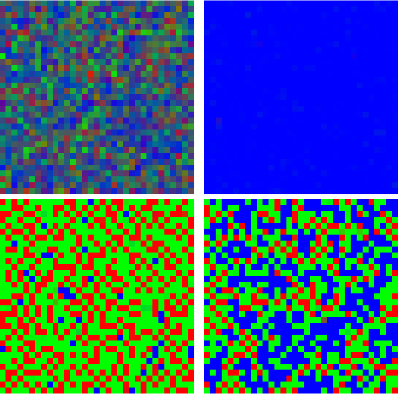
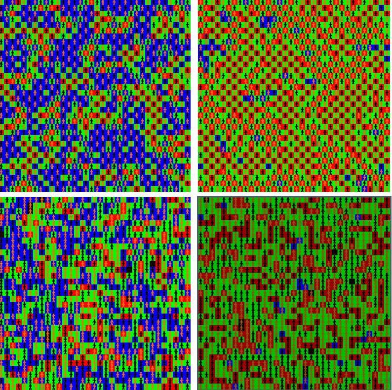
In the disordered phase, \(\beta\), the steepness parameter of the choice function, is low and agents randomly choose a move H, M or L, even for very long periods, say 1 million iteration steps. (see Figure 1 upper left). The pattern of colors keeps fluctuating with colors which are mixtures of red, blue, green reflecting the fact that none of the possible moves H, M or L is preferred by the agents.
Patterns in the ordered regimes
For higher \(\beta/\gamma\) values most cells display pure colors red, blue or green. The agents have strong opinions and always play the same move, H, M or L. As in the well known Schelling (1971, 2006) model of segregation, network interactions increase the initial differences in agent preferences.
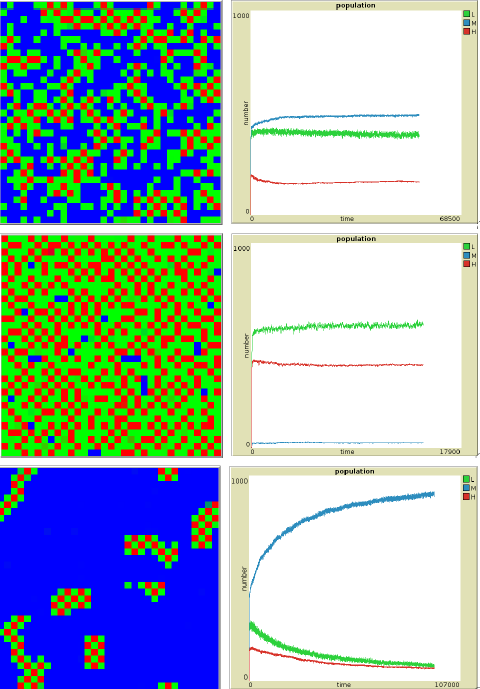
The system self–organises at large iteration times and the lattice gets divided into spatial domains. One attractor type is displayed into one domain. For instance, in the “fair" domain type, all agents always play M (see Figure 1 upper right). Other domains display “unfair configurations" such as agents playing H interact with agents playing L. Both types of domains can coexist on the lattice and remain fixed. Their respective importance depends upon initial conditions: if they favour M moves by spreading \(J_2\) distribution with respect to \(J_1\) and \(J_3\) distributions, as for initial distribution 141, the fair pattern M colored blue occupies most of the lattice (Figure 2 upper plots). Initial distributions such as 414 favour unfair patterns (Figure 2 lower plots).
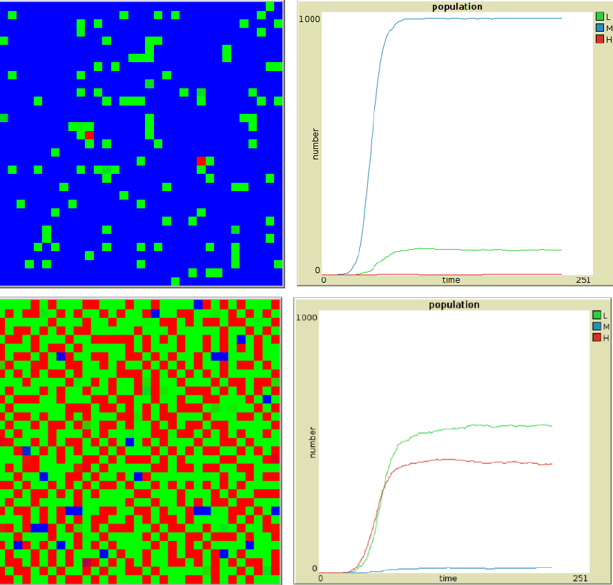
The populations dynamics are displayed on the right plots of Figure 2. Only the populations of agents playing pure strategies is represented. One time unit represent on average 1.68 iterations per agent. The initial increase corresponds to agents increasing their preference towards a pure strategy and the spatial re–arrangement of choices.
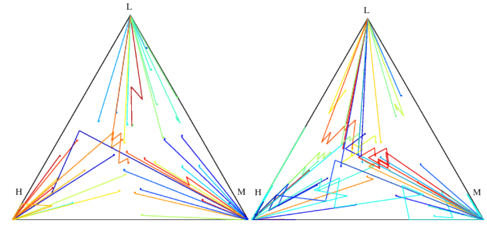
Both processes are displayed when one follows individual \(\bf J\) trajectories on the simplex plots of Figure 3 where the \(\bf J\) dynamics are compared between the full connection topology and the lattice. A three dimension vector such as \(\bf J\) can be represented by its position on the simplex, chosen as the center of gravity of masses proportional to \(J_1,J_2,J_3\) placed at the vertices H,M,L of the simplex. In other words the two coordinates \(J_x, J_y\) in the plan are:
| $$J_x= \frac{J_2+J_3/2}{J_1+J_2+J_3},\ J_y= \frac{\sqrt{3}J_3/2}{J_1+J_2+J_3} $$ | (4) |
Different textures are represented on Figure 4, depending upon agent neighborhood. Von Neumann neighborhood favors bars textures while von Neumann neighborhood allows chessboards.

In fact, for a given value of \(\beta\) the stability of any choice depends upon the magnitude of the unique non–zero preference coefficient:
| $$J_i = \frac{<\pi_i>}{\gamma} $$ | (5) |
| $$P \simeq exp (- \beta J_i) $$ | (6) |
In the chessboard texture, an H playing agent with 4 neighbors playing L would get an average payoff of 0.7.
But with 8 neighbours she would only get 0.35 on average since she gets 0 payoff when playing with her 4 H playing neighbors. While in the bar configuration, H playing agents are surrounded by 6 agents playing L and 2 playing H: their profit is 0.525; bar textures are then more favorable than chessboards in the Moore neighborhood.
Equations (5–6) are the reason for the observed stability of patterns in the multi–phase regime. At equilibrium the probability of changing one agent’s choice is of the order of \(8.10^{-7}\) for H, \(4.10^{-5}\)for M and \(2.10^{-3}\) for L when \(\beta=2\) and \(\gamma= 0.1\). By comparison the probability of such changes in the model of Axtell et al. (2001) are much higher, \(\epsilon=0.1\), which explains why they report transients rather attractors.
The influence of the neighborhood also applies to random networks. H and L payoff and patterns depend in fact upon the parity of the loops the nodes are implied in. Even loops[4] allow the HLHL alternation as in von Neumann neighborhood (see Figure 5, left). However, odd loops such as those present in Moore neighborhood do not (see Figure 5, right). To predict the probability of local textures around a node one can simply check the parity of the loops around it. Odd loops decrease average payoff and thus the probability of alternating H and L configurations.
The analysis is easily performed in the case of small world networks (Watts & Strogatz 1998) with many short loops. Santos et al. (2012) studied small world nets based on one dimensional periodic structures with 3–loops, in other word with large clustering coefficients: they report that this network structure favours support the equity regime in accordance with the above analysis. In small world nets with many 4–loops, the parity of loops is expected to allow inequity attractors.
By contrast, Erdős & Rényi (1960) random nets have very few short loops and parity is less important and paths with alternating H and L choices may appear. The scale free property (Albert & Barabási 2002) is not enough by itself to allow any prediction since it does not say anything about the clustering coefficient which determines the occurrence of 3–loops.
To summarize Section 2 results, ordered phases display spatial domains on lattices, in fair or unfair configurations. Unfair configurations display specific textures depending upon neighborhood. Which phases are observed depends upon parameter \(\frac{\beta}{\gamma}\) and their relative importance depends upon initial conditions.
Phase diagrams: dynamical regimes and transitions
Phase diagrams allow a clearer view of the regimes and patterns obtained according to parameter changes. We have a choice among several quantities to monitor dynamical regimes such as preference coefficients or fractions of agents choices. We present the results obtained by monitoring fractions of agents playing H, L or M in the next figures 6, 7, 11 and 12 but equivalent results are obtained when monitoring the evolution of preference coefficients.
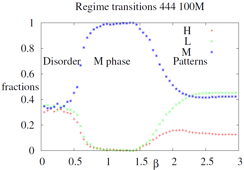
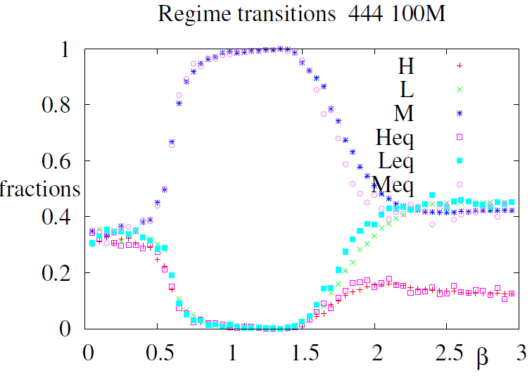
The phase diagram of Figure 6 was obtained by decreasing \(\beta\) from 3.0 to 0.1 . The initial conditions were 444 for \(\beta=3.0\), but equilibria for \(\beta<3.0\) were computed from the previous \(\beta\) equilibrium \(J\) values, e.g the initial conditions to compute equilibrium at \(\beta=2.4\) were the conditions of equilibrium at \(\beta=2.5\), according to the so–called adiabatic procedure[5]. The phase diagram displays the succession of dynamical regimes: the dis-ordered regime displayed on Figure 1 upper left is obtained when \(\beta < 0.5\); an homogeneous regime where all agents play M as displayed on Figure 1 upper right is observed when \(0.5<\beta < 1.5\) and the ordered multi–phase regime as in Figure 1 lower diagrams and Figure 2 is observed when \(\beta> 1.5\).
This diagram is pretty similar to the regime diagram observed for the fully connected networks described in Weisbuch (2018) except that the second phase transition from homogeneous M phase to the ordered multi– phase regime is not abrupt on the lattice. It should also be noted that the decreasing \(\beta\) procedure is not reversible: when \(\beta\) is increased from 0.1 to 3.0 the system remains in the M regime after \(\beta> 1.5\), see Figure 11. This is because the initial conditions for the higher \(\beta\) values are maintained from the M regime: the system displays hysteresis. Both properties are due to the multiplicity of attractors and the metastability of the domain structure to be further analysed in Appendix A.
| L | M | H | |
| L | 0.5-\(\lambda\) | 0.5-\(\lambda\) | 0.5-\(\lambda\) |
| M | 0.5 | 0.5 | 0 |
| H | 0.5+\(\lambda\) | 0 | 0 |
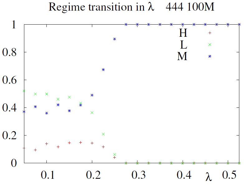
Since we have presently used only one reduced parameter, \(\frac{\beta}{\gamma}\), we can add another one and consider the figures of the payoff matrix as parameters. Keeping the idea of symmetry between demands with respect to 0.5 we introduce the extra parameter \(\lambda\) which we call the inequity parameter. \(\lambda\) is the difference in the payoff matrix between 0.5, the equity payoff and what L and M players get. The previous simulations, Figures 1– 6, were done for \(\lambda=0.2\). The generalised payoff matrix is rewritten in Table 2.
We then obtain a regime diagram in \(\lambda\) (Figure 7) plotted at \(\beta=2.0\) following the fractions of agents playing H, M or L versus \(\lambda\). One only observes the ordered multi–phase regime until \(\lambda \le 0.2\). Above \(\lambda = 0.2\), the smaller payoff obtained when playing L is not sufficient to maintain the stability of the L choice. The fraction of L players starts collapsing and so does the fraction of H players who would make no profit in their absence. Only M players survive and the equity norm is observed. One can connect this feature to the observation that people refuse to accept a too small part of the pie as studied for instance by Henrich et al. (2001) even though economists’ reasoning would predict acceptance of any offer during a one shot game.
Agents with Tags Dynamics
The most significant result in Axtell et al. (2001) concerned agents with tags. Agents are divided into two populations with arbitrary tags say e.g. one orange and one black. When agents take into account tags for playing and memorising games (in other words when each population of agents plays separately two games, one intra–game against agents with the same tag and another inter–game against agents with a different tag) one observes configurations in the inter–game such that one population always play H while the other population plays L; they interpret such inequity norm as the emergence of classes, the H playing population being the upper class.
A first version of the bargaining game with tags on lattice was proposed by Poza et al. (2011) with a minor change with respect to Axtell et al. (2001): agent moves were chosen to respond to the most frequent moves of their opponent rather than optimising the best expected payoff from the whole sequence of game memories. They observed the same regimes as reported by Axtell et al. (2001) or their combination.
A couple of remarks before describing our results:
- Three games independently occur with two tags A and B: A agents play an intra–game against agents A and B against B, and A and B play an inter–game against each other. Since the games are independent we don’t need to give a description of the 3 games altogether. The configuration of agents choices obtained by simulation are the union of the configurations achieved in each game.
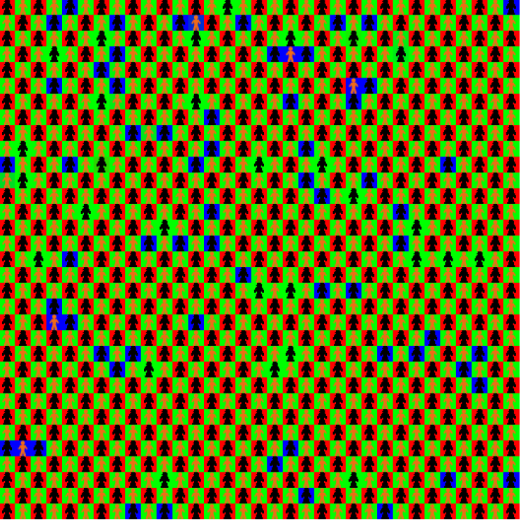
- One can choose among different assignments, random or regular[6], of tagged agents to the cells of the lattice (see Figure 8).
Let us start with the simplest case of regular assignment of tags to cells as obtained by alternation as in Figure 8, right panel. Simulation results for the inter–game, orange versus black agents, are displayed on the two upper panels of Figure 9. Each agent has four neighbours with a different tag to play with. Initial conditions are 444 for the left panel and 414 for the right panel. The chessboard domains are clearly displayed on the right panel: in some domains “orange agents" play H and “black agents" play L, but the opposite is observed in other domains. This situation transcribes the inequity norm proposed by Axtell et al. (2001). Most agents reach their saturation values and their choices remain stable.
The intra–game possible configurations are those described in the previous section for the von Neumann neighbourhood. The lattice panels only have to be rotated by 45 degrees since neighbours for intra–games are now along diagonals.
When one starts from initial conditions with black tag agents playing mostly H and orange tag agents playing mostly L, the initial choices are re–enforced during the iteration and remain stable for 2 000 time steps (Figure 10). One single domain of black agents playing H and orange agents playing L covers most of the lattice with a few exceptions of agents playing M and some black agents playing L.
We also use random assignments of tags to lattice cells with Moore neighborhood since the 8 possible a priori neighbours are restricted to an average of 4 neighbours because only pairs of different agents interact in the inter–game. The same also applies in the intra–games. As compared to the previous simulations of Sections 2.7-2.21 and 2.22-2.26 with von Neumann neighborhood without tags, the average number of neighbours is the same, but the connection structure is more random. Such a choice was already made by Poza et al. (2011).
One indeed observes on the lower plots of Figure 11 some correlation between tags and agent choices, especially when initial conditions such as 414 favour HL domains. But because of network randomness these correlations are short range: there are some regions of the lattice where orange agents play H and black agents play L while the opposite occurs in other regions (see Figure 11 lower right panel). No regular patterns such as chessboards nor bars are observed.
When one starts from initial conditions with black tags playing mostly H and orange tags playing mostly L, the initial choices are re–enforced during the iteration and remain stable for 2 000 time steps (Figure 10). One single domain of black agents playing H and orange agents playing L covers most of the lattice with a few exceptions of agents playing M and some black agents playing L.
Discussion and Conclusions
Let first discuss the main differences between Axtell et al. (2001), Poza et al. (2011) and Santos et al. (2012) and the present work. Since they use different memorisation and choice function, one is not surprised to get some difference in behaviour. They observe long transient regimes which they interpret as norms of behaviour while we rather observe attractors. Previous papers report the observation of “a fractious regime (FR), in which agents alternate their demands between H and L" (Poza et al. 2011). We never observe such a regime. This discrepancy comes from the difference between attractors observed in our BOMA dynamics and their transient regimes due to their choice of a relatively large and constant probability of random transitions.
Another important difference is that once the equity norm is established at large \(\beta\) value it remains stable even under parameter values which would support inequity. History admittedly provides examples of transitions from more equitable situations to inequity such as slavery: to model such transitions in a BOMA perspective, one would have to add some processes to the model such as wars and invasions which indeed were at the origin of slavery
Our most significant result is the fact that the inequity norm can be observed on lattices even in the absence of tags. The restriction of game partners to a few and the short loops of interaction foster its emergence. The same reasoning applies to more random connection structures with short interaction loops. Interpreting this result in real societies means that we might expect the possibility of the inequity norm in strongly structured societies where the social network dominates who interacts with whom. The fact that tags are not a necessary condition for inequity on lattices does not deny their role in human societies as first stressed by Axtell et al. (2001). Racism and its consequences can certainly be interpreted in this framework. During the Middle Ages, some societies have even imposed tags such as specific garments to some of their members to discriminate against them, e.g. against Jews and against lepers. Tags and discrimination can certainly play a role in more anonymous modern and larger societies.
The fact that large \(\gamma\) values drive the system towards the equity norm (see Figure 5) means that equity is favoured by forgetting[7]. This property can be related to the role of forgiveness in re–establishing cooperation in the prisoner dilemma game as reported in Axelrod (1997a).
We have also seen (see Figure 7) that too much greed can destabilize the inequity norm and bring back equity, a prediction to compare with ethnological data (Henrich et al. 2001) and the History of Revolutions.
We only have scratched the surface of the problem of inequity in social networks. The lattice connection structure is only a toy model of a social network. However, it still allowed us to predict the influence of loops’ parity on possible local arrangements of H and L agents. These predictions should be actually tested on various versions of social nets from trees and random graphs to small world and diverse scale free networks. Another possible continuation of the present work could be to introduce a “slow dynamics" on parameters or a small “seed" domain of “opponents"[8] to check the spatio–temporal dynamics of “revolutions" of both kinds, either towards equity or inequity.
Acknowledgements
We thank Sophie Bienenstock, Bernard Derrida and Laya Ghodrati for helpful discussions and three anonymous referees for suggestions.Notes
- This result is rigorous only in the Mean Field approximation.
- The average is done at equilibrium on games against the agent’s neighbours.
- The approximate value of \(P\) in Equation 6 is obtained by neglecting in Equation 2 the other two exponentials with small exponents with respect to the main term \(exp(\beta. J_i)\). When \(\beta=2, \gamma= 0.1, \pi=0.7\) the ratio is \(1.2\,10^6\).
- The relevant notion is the balance of a signed graph, a concept introduced by Harary (1953) and later called frustration by Toulouse (2014). Frustrated loops are unbalanced signed graphs. A loop of negatively interacting elements has no stable configuration when the number of elements is odd. This applies to H choices which are only stable when connected to L choices.
- The adiabatic procedure consists in following the system equilibrium when parameters such as \(\beta\) and \(\gamma\) are slowly varied. An alternative procedure is to compute equilibrium values from the same initial conditions. Both diagrams display little difference, see Figure 13 in the Appendix A.
- And many more, such as bilayer nets.
- \(\gamma\) is the time rate at which agents forget their past profits.
- For instance a small domain of agents playing M among a much larger domain of H/L playing agents to represent revolutions.
Appendix
A: Transition diagrams
The generic properties of the transition diagram of Figure 6, i.e. the succession of disordered, fair and multi-phase regimes with the increasing values of \(\frac{\beta}{\gamma}\) are preserved when minor changes are performed.
Size effects such as increasing the size of the lattice from 10x10 to 33x33 and to 100x100 while maintaining constant the number of games per agent (\(2. 10^5\)) do no modify the phase diagram.
We also tested changes in neighborhood, initial conditions, direction of the changes in \(\frac{\beta}{\gamma}\) etc. No change of the variation of fractions of choices HLM is observed in the disordered phase and in the intermediate parameter region where all agents choose M. Changes only concern the multi–phase region which may start above \(\beta=1.25\).
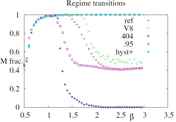
The influence of these factors are checked on Figure 11. One factor at a time is changed. They are:
- Changing the neighborhood from von Neumann to Moore. The observed decrease of stability of the HL domain for M8 neighborhood is due to the decrease of \(J_1\) in bar patterns as earlier discussed: the average payoff for H is only 0.525 instead of 0.7 for vN4 neighborhood.
- Changing initial conditions from uniform 444 to 404, thus lowering the early proportion of M agents, reduces the M playing domain.
- Changing \(\gamma\) to 0.05 instead of 0.1 while keeping the \(\beta/\gamma\) ratio constant. The stability of the HL domain is increased when \(\gamma=0.05\) instead of 0.1 since the same decrease of the \(J_1\) and \(J_3\) needs twice as many consecutive alternative changes as when \(\gamma=0.1\)
- Increasing \(\beta\) from 0.5 to 2.5 rather than decreasing it, as done for all other transitions diagrams, maintains the system in the fair attractor. Since the initial conditions are “fair" when \(\beta\) is increased above 1.2, the system carries on following the fair attractor when one further increases \(\beta\). The increasing and decreasing branches of the diagram are then identical when \(\beta < 1.2\) but differ above 1.2.
The observed changes with obvious explanations are those due to the change of initial conditions in the multiphase domains, namely when \(\beta\) is increased and when non–uniform initial conditions 404 are chosen. The width of the transition and its translation for different conditions are due to the metastability of the domains in the close neighborhood of the transition i.e. when \(\beta \simeq. 1.5\). In that region the M phase is a strong attractor and would predominate over the H/L phase at infinite iteration time. We monitored the slow erosion of the H/L domain and its invasion by the M domain when \(\beta = 1.5\) on Figure 12 during 100,000 time steps corresponding to 100,000 iterations per agent. One can observe during the simulations that the “blue" phase of M players dissolve gradually the H/L regions starting with the irregularities of chessboard pattern until only the most regular patterns survive at large iteration times. By contrast, when \(\beta=2\) farther from the transition, the relative stability of the H/L phase is preserved.
Increasing the number of games per agent from \(2. 10^5\) to \(2. 10^6\) and to \(2. 10^7\) increases the size of equity region: the transition in \(\beta\) from equity to mixed attractors is increased from 1.4 to 1.6 and to 1.8. This is one more indication that the equity attractor is the most stable and that it would be reached if the game would continue forever.
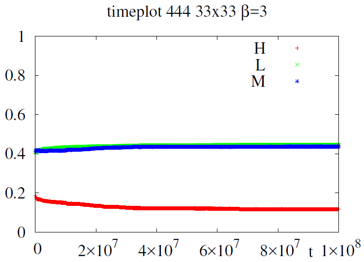
The stability of the multiphase attractor for larger \(\beta\) values \(\beta=3\) can be observed on the time plot of Figure 13 with \(\beta=3\).
The above regime diagrams (fig. 6,7,11) were measured following “adiabatic decay": initial conditions were applied to measure \(\bf J\) at the highest \(\beta/\gamma\) value, i.e. the rightmost points, and the obtained equilibrium values were kept to initiate the computation of next point, and so on. Another method is to compute each point from the same initial conditions. Figure 14 shows that the curves display very little difference.
B: Simulation software
We used NetLogo (Wilensky 1999) version 6.0.2 software to run single simulations which results are displayed on Figures 1, 2, 4, 9, 10 and 12.
The program is available as https://github.com/weisbuch/inequity.f/blob/master/BMnov.nlogo
The simplex trajectories Figure 3, the transition diagrams Figures 6, 7, 11 and 14 and the time plots of Figure 13 were obtained by a fortran program available as https://github.com/weisbuch/inequity.f/blob/master/transforjasss.f The corresponding figures were drawn using gnuplot. The simplex trajectories of Figure 3 were drawn directly from the fortran program to generate the PostScript file.
The NetLogo program allows to simply choose parameters and set–up, to run simulations and to observe evolving patterns and the dynamics of agent choices. The FORTRAN program runs faster and is well adapted to check transition diagrams after long iteration times. Having two independent programs also allows a further check for programming errors.
References
ACKLEY, D. H., Hinton, G. E. & Sejnowski, T. J. (1985). A learning algorithm for Boltzmann machines. Cognitive Science, 9(1), 147–169. [doi:10.1207/s15516709cog0901_7]
ALBERT, R. & Barabási, A.-L. (2002). Statistical mechanics of complex networks. Reviews of Modern Physics, 74(1), 47.
ANDERSON, S. P., De Palma, A. & Thisse, J. F. (1992). Discrete Choice Theory of Product Differentiation. Cambridge, MA: MIT Press.
AXELROD, R. (1997a). The dissemination of culture a model with local convergence and global polarization. Journal of Conflict Resolution, 41(2), 203–226.
AXELROD, R. M. (1997b). The Complexity of Cooperation: Agent-Based Models of Competition and Collaboration. Princeton, NJ: Princeton University Press.
AXTELL, R. L., Epstein, J. M. & Young, H. P. (2001). 'The emergence of classes in a multiagent bargaining model.' In S. N. Durlauf & H. Peyton Young (Eds.), Social Dynamics, (pp. 191–211). Cambridge, MA: MIT Press.
BONABEAU, E., Theraulaz, G. & Deneubourg, J.-L. (1995). Phase diagram of a model of self-organizing hierarchies. Physica A: Statistical Mechanics and its Applications, 217 (3), 373–392. [doi:10.1016/0378-4371(95)00064-E]
BOUCHAUD, J. P. (2013). Crises and collective socio-economic phenomena: simple models and challenges. Journal of Statistical Physics, 151(3-4), 567–606.
BOWLES, S. & Naidu, S. (2006). Persistent institutions. Santa Fe Institute Working paper, 08(04).
CASTELLANO, C., Fortunato, S. & Loreto, V. (2009). Statistical physics of social dynamics. Reviews of Modern Physics, 81(2), 591.
EPSTEIN, J. M. (2006). Generative Social Science: Studies in Agent-Based Computational Modeling. Princeton, NJ: Princeton University Press.
ERDŐS, P. & Rényi, A. (1960). On the evolution of random graphs. Publications of the Mathematical Institute of the Hungarian Academy of Sciences, 5(1), 17–60.
HARARY, F. (1953). On the notion of balance of a signed graph. The Michigan Mathematical Journal, 2(2), 143–146. [doi:10.1307/mmj/1028989917]
HENRICH, J., Boyd, R., Bowles, S., Camerer, C., Fehr, E., Gintis, H. & McElreath, R. (2001). In search of homo economicus: Behavioral experiments in 15 small-scale societies. The American Economic Review, 91(2), 73–78.
HOPFIELD, J. J. (1982). Neural networks and physical systems with emergent collective computational abilities. Proceedings of the National Academy of Sciences of the United States of America, 79(8), 2554–2558. [doi:10.1073/pnas.79.8.2554]
NADAL, J.-P., Weisbuch, G., Chenevez, O. & Kirman, A. (1998). A formal approach to market organization: Choice functions, mean field approximation and maximum entropy principle. Advances in self-organization and evolutionary economics, Economica, London, (pp. 149–159).
NASH Jr, J. F. (1950). The bargaining problem. Econometrica, 18(2), 155–162. [doi:10.2307/1907266]
PARETO, V. (1896). Cours d’économie politique professé à l’Université de Lausanne, vol. 1. Lausanne: F. Rouge.
POZA, D. J., Santos, J. I., Galán, J. M. & López-Paredes, A. (2011). Mesoscopic effects in an agent-based bargaining model in regular lattices. PLoS ONE, 6(3), e17661. [doi:10.1371/journal.pone.0017661]
RUMELHART, D. E., McClelland, J. L. & PDP Research Group (1987). Parallel Distributed Processing, Volume 1. Cambridge, MA: MIT Press.
SANTOS, J. I., Poza, D. J., Galán, J. M. & López-Paredes, A. (2012). Evolution of equity norms in small-world networks. Discrete Dynamics in Nature and Society, 482481. [doi:10.1155/2012/482481]
SCHELLING, T. C. (1971). Dynamic models of segregation. Journal of Mathematical Sociology, 1(2), 143–186.
SCHELLING, T. C. (2006). Micromotives and Macrobehavior. New York, NY: W.W. Norton.
SKYRMS, B. (2014). Evolution of the Social Contract. Cambridge: Cambridge University Press.
TOULOUSE, G. (2014). Theory of the frustration effect in spin glasses: I. In Spin Glass Theory and Beyond, (pp.99–103). Singapore: World Scientific.
WATTS, D. J. & Strogatz, S. H. (1998). Collective dynamics of ’small-world’ networks. Nature, 393(6684), 440–442.
WEISBUCH, G. (2018). Persistence of discrimination: Revisiting Axtell, Epstein and Young. Physica A: Statistical Mechanics and its Applications, 492(Supplement C), 39–49. [doi:10.1016/j.physa.2017.09.053]
WEISBUCH, G., Kirman, A. & Herreiner, D. (2000). Market organisation and trading relationships. The Economic Journal, 110(463), 411–436.
WILENSKY, U. (1999). NetLogo. Center for Connected Learning and Computer-Based Modeling, Northwestern University. Evanston, IL.
YOUNG, H. P. (1993). An evolutionary model of bargaining. Journal of Economic Theory, 59(1), 145–168.