
Introduction
Brief Review
Game theory is a mathematical system for analyzing and predicting how humans behave in strategic situations. It uses three distinct concepts to make precise predictions of how people will, or should, interact strategically: strategic thinking, best-reply, and mutual consistency (equilibrium). Strategic thinking assumes that all players form beliefs based on an analysis of what other players may possibly do. The best-reply chooses the best reply given those beliefs. Mutual consistency adjust best responses and beliefs until they reach an equilibrium. In this sense, there is an understandable interest in the development and implementation of interaction social models which tries to understand, predict, manipulate and control the behavior of people, organizations, government, companies, etc. for instance, see Schindler (2012), Xianyu (2010), Wijermans et al. (2013). Everyone that goes aboard on this kind of interaction models must consider the behavior observations of the fifteenth-century philosopher and politic, Niccolò Machiavelli (Wilson et al. 1996).
Machiavelli's primary contribution was his painfully honest observations about human nature Machiavelli (1952). He distinguishes the natural laws that govern how effective leaders exercise power over the human resources and creates a new moral system, deeply rooted in Roman virtue (and vice). He develops his proposal against the conceptions of the Judeo-Christian self-contained moral systems. His ethical system works both as a limit to human possibilities and as the source of human virtue. Machiavelli says that human nature is aggressive and only in some measure able to be manipulated. In this sense, he observes that under competitive conditions the human bean pursue his main goals with increasing levels of ruthlessness (Machiavelli 1952; Machiavelli 1965; Machiavelli 2001).
It is important to note that Machiavelli showed consideration for moral individuals (Leary et al. 1986), and recognized that exist individuals able to sacrifice their own self-interest in order improve the interests of others. However, he did question the regular occurrence of self-sacrifice and ideal altruism behavior in the real world.
A Machiavellian individual (Calhoun 1969) is one who employs aggressive, manipulative, exploiting and devious moves in order to achieve personal and organizational objectives. These moves are undertaken according to perceived feasibility with secondary consideration (what is necessary under circumstances) to the feelings, needs and/or rights of others.
Although most of what Machiavelli had to say was intended to provide advice on how successful leaders exercise power over political organizations, his views can (and should) be applied to today's business executives and organizations, given that all organizations are subject to power politics. Machiavelli believed that all leaders deal with the fact that human beings compete for power. Therefore, it makes sense for leaders to see themselves as engaged in two different conflicts: internal and external with "followers" and "competitors" (Wilson et al. 1996).
Machiavellianism is defined as follows:
Definition 1
Machiavellianism is a social conduct strategy supposing that the world can
be manipulated by applying (Machiavelli's) tactics with the purpose of
achieving personal gains according (or not) to a conventional moral.
For the purposes of this paper, we will consider the terms views, tactics and immorality defined as follows:
- Views: The belief that the world can be manipulated - the world consists of manipulators and manipulated
- Tactics: The use of a manipulation strategies needed to achieve specific power situations (goals). Strategies are analyzed in Machiavelli's The Prince (Machiavelli (1965), The Discourses (Machiavelli (1965), The Art of War (Machiavelli 2001) and the psychological behavior patterns (described above).
- Immorality: The disposition to not become attached to a conventional moral.
The Machiavellian intelligence is the capacity of an individual to be in a successful engagement with social groups (Byrne and Whiten 1988).
Machiavellianism and moral behavior
Machiavellianism has been associated with different variables, given a wide range of interpretations related to psychological components (Byrne and Whiten 1988). Smith (1979) argued that the descriptors of the psychopath and those of the Machiavellian must have common domains, because of their similarity (manipulative style, poor affect, low concern about conventional moral, low ideological compromise, and others). In agreement with Cleckley (1976), other Machiavellian tendencies coincide with some components of anomie (cynicism, low interpersonal credibility, external locus of control).
Researchers have investigated the relationship between locus of control and Machiavellianism. Solar and Bruehl (1971 ) were the first in establishing a relationship between Machiavellianism and locus of control, considering both as aspects of interpersonal power. Their study reported a significant relationship between Machiavellianism and external locus of control for males, but not for females. Prociuk and Breen(1976) supported this result. Mudrack (1989) conducted a meta-analytic review of 20 studies determining the relationship between Machiavellianism and external locus of control. Gable et al. (1992) sustain this result. They related locus of control, Machiavellianism and managerial achievement; their results did not show significant correlations between locus of control and achievement, but found a positive correlation between Machiavellianism and external control.
With respect to influence tactics, Falbo (1977) showed that persons with high Machiavellianism are associated with the use of rational indirect tactics (i.e., lies), while those with low Machiavellianism are associated with the rational use of direct tactics (i.e. rewards). Grams and Rogers (1990) research confirms this result and also shows that persons with high Machiavellianism are more flexible when it comes to breaking some ethical rules. Vecchio & Sussmann (1991) suggested that Machiavellianism and the tactics selection are related to sex and organizational hierarchy; the use of influence tactics is common in males and females with high-level positions.
In accordance with different studies of social psychology, manipulation is placed among the forms of social influence as part of the social conduct behavior. Raven (1993) argued that power can be psychologically studied as a product of behavior, including personal attributes, with the possibility to affect others through interaction, and the environment structure. Dawkins (1976) proposed that, in terms of selfishness, altruism, cooperation, manipulation, lie and truth, genetically there exists a selfishness and manipulation gene. Dawkins & Krebs (1978) classified manipulation as a natural-selection state benefiting individuals able to manipulate others' behavior. Vleeming (1979) denoted a personality dimension in which people can be classified in terms of being more or less manipulated in different interpersonal situations. Wilson et al. (1996) defined Machiavellianism as a social strategy behavior involving the manipulation of others to obtain personal benefits, frequently against others' interests. They clarify that anybody is able to manipulate others to different degrees, and they also explain that selfishness and manipulation are behaviors widely studied in evolutionary biology. Hellriegel et al. (1979) defined Machiavellianism as a personal style of behavior in front of others, characterized by: the use of astuteness, tricks and opportunism in interpersonal relationships; cynicism towards other persons' nature; lack of concern with respect to conventional morals. Christie and Geis (1970) proposed three factors to evaluate high or low Machiavellianism: tactics, morality and views. Tactics are concerned with planned actions (or recommendations) to confront specific situations with the purpose of obtaining planned benefits at the expense of others. Morality is related to behavior that can be associated with some degree of "badness" with respect social conventions. Views involve the idea that the world consists of manipulators and manipulated. In this sense we introduce the following definition.
Immorality is a un-arrangement of customs. One of the best-known concepts is the immorality described by Nietzsche. Therefore, we consider the factor of morality proposed by Christie and Geis (1970) as inappropriate, because in the evaluation of the factor, immorality is considered the opposite to a "conventional moral."
There have been proposed several methods from different angles and application domains for solving the problem of moral and ethical decision making (Bales 1971; Cervantes et al. 2011; Dehghani et al. 2008; Indurkhya and Misztal-Radecka 2016; Wallach et al. 2010; Hartog and Belschak 2012). However, there is still a lack of a fundamental and mathematical decision model and a rigorous cognitive process for decision-making. In this paper, we will propose a game theory solution combined with a reinforcement learning approach to acquire manipulation behavior.
Main results
This paper presents a new game theory approach for modeling manipulation behavior based on the Machiavellian social conduct theory. The Machiavellian game conforms a system that allows to analyze and predict how Machaivellian players behave in strategic situations combining all the following three fundamental features of game theory: a) formation of beliefs based on analysis of what others players might do (strategic thinking); b) choosing a best-reply given those beliefs (optimization); and c) adjustment of best-reply and beliefs until they are mutually consistent (equilibrium). The assumption of mutual consistency is justified by introducing a learning process. As a result, the Machiavellian equilibrium is the consequence of a strategic thinking, optimization, and equilibration (learning process).
A Machiavellian player conceptualizes the manipulation social conduct considering three concepts: views, tactics and immorality. For modeling the Machiavellian Views and Tactics we employ a Stackelberg/Nash game theory approach. For representing Machiavellian immorarilty we introduce utilitarian and deontological moral theories and we review psychological findings regarding moral decision making (Tobler et al. 2008). An advantage of the Machiavellian social conduct theory is that whereas other moral theories provide standards for how we should act, they do not describe how moral judgments and decisions are achieved in practice. Next, we establish a relationship between moral behavior and game theory (economic theories) and we suggest a reinforcement learning approach which provides evidences of how people acquire Machiavellian immoral behavior, considering its principle of error-driven adjustment of cost/reward predictions.
In summary, this paper makes the following contributions:
- We represent the Machiavellian Views naturally as a Stackelberg game where the hierarchical organization consists of manipulators (leaders) and manipulated (followers) players. By definition of the Stackelberg game the leaders have commitment power.
- The manipulators and manipulated players are themselves in a (non-cooperative) Nash game.
- The Machiavellian Tactics correspond to the solution of Stackelberg/Nash game.
- We employ the extraproximal method for solving the Machiavellian game (Antipin 2005; Trejo et al. 2015, 2016 ) (see the appendix).
- We suggest a reinforcement learning approach for modeling the Machiavellian immorality based-on an Actor-Critic architecture
- For representing the Machiavellian immorality, we consider that rational players employ deontological and utilitarian moral (depending the case)
- We suggest the immorality reinforcement learning rules needed for modeling immorality.
- We restrict our approach to a finite, ergodic and controllable Markov chains.
- The result of the model is the manipulation equilibrium point.
- Finally, we present a numerical example that validates the effectiveness of the proposed Machiavellian social conduct and intelligence approach.
Organization of the paper
The rest of the paper is organized as follows. In the next Section, we present the mathematical background needed for the understanding of the rest of the paper. Section 3 describes the general Machiavellianism social conduct architecture. We suggest a Machiavellian Stackelberg game theory model for representing Machiavellian Views and Tactics, in Section 4. Section 5 describes a reinforcement learning approach for modeling the Machiavellian immorality. In Section 6, we present a simulated experiments for Machiavellian social conduct theory. Finally, in Section 7 we present some conclusions and future work. To make the paper more accessible, the long details needed to implement the extraproximal method are placed in the appendix.
Preliminaries
Let \(S\) be a finite set, called the state space, consisting of finite set of states \(\left\{ s_{\left( 1\right) },...,s_{\left( N\right)}\right\}\) , \(N\in \mathbb{N}\). A Stationary Markov chain (Clempner & Poznyak 2014) is a sequence of \(S\)
-valued random variables \(s(n),\) \(n\in \mathbb{N}\). The Markov chain can be represented by a complete graph whose nodes are
the states, where each edge \((s_{(i)},s_{(j)})\in S^{2}\) is labeled by the
transition probability. The matrix \(\Pi =(\pi _{(ij)})_{(s(i),s(j))\in S}\in
\lbrack 0,1]^{N\times N}\) determines the evolution of the chain: for each \(k\in \mathbb{N}\), the power \(\Pi ^{k}\) has in each entry \((s_{(i)},s_{(j)})\) the
probability of going from state \(s_{(i)}\) to state \(s_{(j)}\) in exactly \(k\)
steps.
Definition 2
A controllable Markov chain (Poznyak et al. 2000) is a 4-tuple
| $$ MC=\{S,A,\mathbb{K},\Pi \}\label{MC} $$ | (1) |
- \(S\) is a finite set of states, \(S\subset \mathbb{N}\), endowed with discrete a topology;
- \(A\) is the set of actions, which is a metric space. For each \(s\) in S, \(A(s)\subset A\) is the non-empty set of admissible actions at state \(s\in S\). Without loss of generality we may take \(A\mathbf{=\cup }_{s\in S}A(s)\);
- \(\mathbb{K}=\left\{ (s,a)|s\in S,a\in A(s)\right\}\) is the set of admissible state-action pairs, which is a measurable subset of \(S\times A\);
- \(\Pi =\left[ \pi _{(ij|k)}\right]\) is a stationary controlled transition matrix, where
represents the probability associated with the transition from state \(s_{(i)}\) to state \(s_{(j)}\) under an action \(a_{(k)}\in A(s_{(i)}),\) \(k=1,...,M\);$$ \pi _{(ij|k)}\equiv P(s(n+1)=s_{(j)}|s(n)=s_{(i)},a(n)=a_{(k)}) $$
| $$ MDP=\{MC,J\}\label{MD} $$ | (2) |
- MC is a controllable Markov chain (Eq. 1)
- \(J:S\times \mathbb{K}\rightarrow \mathbb{R}\) is a cost function, associating to each state a real value.
The strategy (policy)
| $$ d_{(k|i)}(n)\equiv P(a(n)=a_{(k)}|s(n)=s_{(i)}) $$ |
The elements of the transition matrix for the controllable Markov chain can be expressed as
| $$ \begin{array}{c} P\left( s(n+1)=s_{(j)}|s(n)=s_{(i)}\right) = \sum\limits_{k=1}^{M}P\left( s(n+1)=s_{(j)}|s(n)=\\ s_{(i)},a(n)=a_{(k)}\right) d_{(k|i)}(n) \end{array} $$ |
Let us denote the collection \(\left\{ d_{(k|i)}(n)\right\}\) by \(D_{n}\) as follows
| $$ D_{n}=\left\{ d_{(k|i)}(n)\right\} _{k=\overline{1,M},\text{ }i=\overline{1,N }} $$ |
A policy \(\left\{ d_{n}^{loc}\right\} _{n\geq 0}\) is said to be local optimal if for each \(n\geq 0\) it maximizes the conditional mathematical expectation of the utility function \(J(s_{n+1})\) under the condition that the history of the process
| $$ F_{n}:=\{D_{0},P\left\{ s_{0}=s\left( j\right) \right\} _{j=\overline{1,N} };...;D_{n-1},P\left\{ s_{n}=s\left( j\right) \right\} _{j=\overline{1,N}}\} $$ |
| $$ d_{n}^{loc}:=\arg {\min_{d_{n}\in D_{n}}}\quad \mathsf{E}\left\{ J(s_{n+1})\mid F_{n}\right\}\label{loc-opt-policy} $$ | (3) |
The dynamics of the Stackelberg game for Markov chains is described as follows. The game consists of \(\iota =\overline{1,\mathcal{M+N}}\) players and begins at the initial state \(s^{\iota }(0)\) which (as well as the states further realized by the process) is assumed to be completely measurable. Each player \(\iota\) is allowed to randomize, with distribution \(d_{(k|i)}^{\iota }(n)\), over the pure action choices \(a_{(k)}^{\iota }\) \(in\) \(A^{\iota }\left( s_{(i)}^{\iota }\right)\), \(i=\overline{1,N_{\iota }}\) and \(k=\overline{1,M_{\iota }}\). The leaders correspond to \(l\) \(=\) \(%\) \(\overline{1,\mathcal{N}}\) and followers to \(m=\overline{1,\mathcal{M}}\). At each fixed strategy of the leaders \(d_{(k_{l}|i_{l})}^{l}(n)\) the followers make the strategy selection \(d_{(k_{m}|i_{m})}^{m}(n)\) trying to realize a Nash-equilibrium. Below we will consider only stationary strategies \( d_{(k|i)}^{\iota }(n)=d_{(k|i)}^{\iota }\). In the ergodic case when all Markov chains are ergodic for any stationary strategy \(d_{(k|i)}^{\iota}\) the distributions \(P^{\iota }\left( s^{\iota }(n+1){\small =}s_{(j_{\iota})}\right)\) exponentially quickly converge to their limits \(P^{\iota}\left( s=s_{(i)}\right)\) satisfying
| $$ P^{\iota }\left( s_{(j_{\iota })}\right) {\small =}\sum\limits_{i_{\iota }=1}^{N_{\iota }}\left( \sum\limits_{k_{\iota }=1}^{M_{\iota }}\pi _{(i_{\iota },j_{\iota }|k_{\iota })}^{\iota }d_{(k_{\iota }|i_{\iota })}^{\iota }\right) P^{\iota }\left( s_{(i_{\iota })}\right) \label{st-distr} $$ | (4) |
The cost function of each player, depending on the states and actions of all the other players, is given by the values \(W_{(i_{1},k_{1};...;i_{\mathcal{ N+M}},k_{\mathcal{N+M}})}^{\iota }\), so that the "average cost function" \(\mathbf{J}^{\iota }\) in the stationary regime can be expressed as
| $$ \begin{array}{c} \mathbf{J}^{\iota }\left( c^{1},..,c^{\mathcal{M+N}}\right) {\small :=} {\small \sum\limits_{i_{1},k_{1}}...\sum\limits_{i_{\mathcal{M+N}},k_{ \mathcal{M+N}}}W_{(i_{1},k_{1},..,i_{\mathcal{M+N}},k_{\mathcal{M+N} })}^{\iota }\prod\limits_{\iota =1}^{\mathcal{M+N}}c_{(i_{\iota },k_{\iota })}^{\iota }} \end{array} \label{loss-functions} $$ | (5) |
| $$ {\small c}_{(i_{\iota },k_{\iota })}^{\iota }=d_{(k_{\iota }|i_{\iota })}^{\iota }P^{\iota }\left( s^{(\iota )}{\small =}s_{(i_{\iota })}\right) \label{c} $$ | (6) |
| $$ c^{(\iota )}\in C_{adm}^{(\iota )}{\small =}\left\{ \begin{array}{c} c^{(\iota )}:\sum\limits_{i_{\iota },k_{\iota }}{\small c}_{(i_{\iota },k_{\iota })}^{\iota }{\small =}1,\text{ }{\small c}_{(i_{\iota },k_{\iota })}^{\iota }{\small \geq }0, \\ \\ \sum\limits_{k_{\iota }}{\small c}_{(j_{\iota },k_{\iota })}^{\iota }{\small =}\sum\limits_{i_{\iota },k_{\iota }}\pi _{(i_{\iota },j_{\iota }|k_{\iota })}^{\iota }{\small c}_{(i_{\iota },k_{\iota })}^{\iota } \end{array} \right.\label{Cadm} $$ | (7) |
| $$ \begin{array}{c} {\small W_{(i_{1},k_{1},..,i_{\mathcal{M+N}},k_{\mathcal{M+N}})}^{\iota }=} \\ \\ {\small \sum\limits_{j_{1}}..\sum\limits_{j_{\mathcal{M+N}}}}J{\small _{(i_{1},j_{1},k_{1},..,i_{\mathcal{M+N}},j_{\mathcal{M+N}},k_{\mathcal{M+N} })}^{\iota }}\prod\limits_{\iota =1}^{\mathcal{M+N}}\pi _{(i_{\iota }j_{\iota }|k_{\iota })}^{\iota } \end{array} $$ |
Notice that by last equation it follows that
| $$ \begin{array}{ccc} P^{\iota }\left( s_{(i_{\iota })}\right) {\small =}\sum\limits_{k_{\iota }}c_{(i_{\iota },k_{\iota })}^{\iota } && d_{(k_{\iota }|i_{\iota })}^{\iota }{\small =}\frac{c_{(i_{\iota },k_{\iota })}^{\iota }}{ \sum\limits_{k_{\iota }}c_{(i_{\iota },k_{\iota })}^{\iota }} \end{array} \text{ }\label{P,d} $$ | (8) |
Let us introduce the variables
| $$ u^{l}:=col\text{ }\left( c^{(l)}\right) ,\text{ }U^{l}:=C_{adm}^{(l)}\text{ } \left( l=\overline{1,\mathcal{N}}\right) ,\text{ }U:=\bigotimes \limits_{l=1}^{\mathcal{N}}U^{l} $$ |
| $$ v^{m}:=col\mbox{ }c^{(m)},\text{ }V^{m}:=C_{adm}^{(m)}\text{ }\left( m= \overline{1,\mathcal{M}}\right) ,\text{ }V:=\bigotimes\limits_{m=1}^{ \mathcal{M}}V^{m}\label{x,v variables} $$ | (9) |
We consider a Stackelberg game where the leaders and the followers do not cooperate. Then, the definitions of the equilibrium point is as follows:
A Stackelberg/Nash equilibrium for the leaders is a strategy \(u^{\ast \ast }=\left( u^{1\ast \ast },..,u^{\mathcal{N\ast \ast }}\right)\) given the fixed strategy \(v=\left( v^{1},..,v^{\mathcal{M}}\right)\) of the followers such that there does not exist any \(u^{l}\in U,\) \(u^{l}\neq u^{l\ast \ast}\).
| $$ \mathbf{J}\left( u^{1\ast \ast },..,u^{l},...,u^{\mathcal{N\ast \ast } }|v\right) \leq \mathbf{J}\left( u^{1\ast \ast },..,u^{\mathcal{N\ast \ast }}|v\right) $$ |
A Stackelberg/Nash equilibrium for the followers is a strategy \(v^{\ast}=\left( v^{1\ast },..,v^{\mathcal{M\ast }}\right)\) given the strategy \(u=\left( u^{1},..,u^{\mathcal{N}}\right)\) for the followers such that
| $$ \mathbf{J}\left( v^{1\ast },..,v^{\mathcal{M\ast }}|u\right) \geq \mathbf{J} \left( v^{1\ast },..,v^{m},...,v^{\mathcal{M\ast }}|u\right) $$ |
Machiavellianism architecture
This paper presents a new game theory model to represent the Machiavellianism (social conduct and intelligence theory). The Machiavellian social conduct is engaged with manipulating others for personal gain, even against the other's self-interest and the Machiavellian intelligence is the capacity of an individual to be in a successful engagement with social groups (Byrne & Whiten 1988). A Machiavellian agent is one who conceptualize the Machiavellianism considering three concepts: views, tactics and immorality. Views involve the idea that the world consists of manipulators and manipulated (restricting the model to two types of agents). The tactics are concerned the use of manipulation (Machiavelli's) strategies. The immorality is related to the natural behavior to not become restricted to a conventional moral (the Machiavellian agent's behavior is rationally bounded by the immorality). In order to (manipulate) acquire power, survive or sustain a particular position, Machiavellian agents make use of Machiavellian intelligence applying different selfish manipulation strategies, which include looking for control the changes taking place in the environment.
Figure 1 shows the schematic structure of the Machiavellian actor-critic algorithm involving a reinforcement learning process. The learning agent has been split into two separate entities: the actor (game theory) and the critic (value function). The actor coincides with a Stackelberg/Nash game (Stackelberg 2011) that implements the concepts of Views and Tactics of the Machiavellianism. The critic conceptualize the Machiavellian immorality represented by a value function process. The actor is responsible for computing a control strategy \(d_{(\hat{\imath}_{\iota}|k_{\iota})}^{\iota\ast }\), for each player \(\iota\), given the current state \(\hat{\imath}_{\iota}\). The critic is responsible for evaluating the quality of the current strategy by adapting the value function estimate. After a number of strategy evaluation steps by the critic, the actor is updated by using information from the critic. The architecture is described as follows.
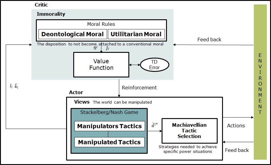
The structure of the game corresponds to a Stackelberg approach in respond to the Machiavellian Views, which involves the idea that the world consists of manipulators and manipulated players. The dynamics of the Machiavellian game is as follows: the manipulators players consider the best-reply of the manipulated players, and then select the strategy that optimizes their utility, anticipating the response of the manipulated players. Subsequently, the manipulated players observe the strategy played by the manipulators players and select the best-reply strategy. The manipulators and manipulated players are themselves in a (non-cooperative) Nash game. Formally, the Stackelberg model is solved to find the subgame perfect Nash equilibrium, i.e. the strategy that serves best each player, given the strategies of the other player and that entails every player playing in a Nash equilibrium in every subgame. The Machiavellian Tactics are concerned with the use of manipulation strategies. In this sense, the equilibrium point of the game represents the strategies needed to achieve specific power situations. In this model, the manipulators have commitment power presenting a significant advantage over the manipulated players.
For representing the concept of immorality we employ a reinforcement learning approach providing a computational mechanism, in which, its principle of error-driven adjustment of cost/reward predictions contributes to the players' acquisition of moral/immoral behavior. The reinforcement learning algorithm is based on an actor-critic approach responsible for evaluating the new state of the system and determine if the cost/rewards are better or worse than expected, supported by the Machiavellian game theory solution. We view actor-critic algorithm as stochastic game algorithm on the parameter space of the actor. The game is solved employing the extraproximal method (see the appendix). The functional of the game is viewed as a regularized Lagrange function whose solution is given by a stochastic gradient algorithm.
The responsibility of the actor is computing the strategy solution \(d_{(\hat{ \imath}_{\iota}|k_{\iota})}^{\iota\ast }\) of the Machiavellian game. In the actor, the action selection follows the strategy solution \(d_{(\hat{\imath} _{\iota}|k_{\iota})}^{\iota\ast }\) of the Machiavellian game: a) given a fixed \(\hat{\imath}_{\iota}\) , each player chooses randomly an action \( a^{\iota}(t)=a_{(\hat{k}_{\iota})}\) (for the estimated value \(\hat{k}\) ) from the vector \(d_{(\hat{\imath}_{\iota}|k_{\iota})}^{\iota\ast }\) , b) then, players employ the transition matrix \(\Pi ^{\iota}=\left[ \pi _{\hat{\imath} _{\iota}j_{\iota}|\hat{k}_{\iota}}^{\iota}\right]\) to choose randomly the consecutive state \(s^{\iota}(t+1)=s_{(\hat{\jmath})}^{\iota}\) (for the estimated value \(\hat{\jmath}\) ) from the vector \(\pi _{(\hat{\imath _{\iota}} j_{\iota}|\hat{k}_{\iota})}^{\iota}\) (for a fixed \(\hat{\imath}_{\iota}\) and \(\hat{k}_{\iota}\) ), c) as soon as \(s^{\iota}(t)\), \(a^{\iota}(t)\) and \(s^{\iota}(t+1)\) are selected they are sent to the Critic.
The role of the critic is to evaluate the current strategy prescribed by the actor and compute an approximation of the projection of \(\hat{\pi}_{(\hat{ \imath},\hat{\jmath}|\hat{k})}^{\iota}(t)\) and \(\hat{J}_{(\hat{\imath},\hat{ \jmath}|\hat{k})}^{\iota}(t)\) . The actor uses this approximation to update its strategies in the direction of performance improvement of the Machiavellian game. In the Critic, we consider that rational Machiavellian players employ a combination of the deontological and utilitarian moral rules, as well as, moral heuristics, for representing the concept of immorality decision-making in the Machiavellianism social conduct theory. Most of the time a Machiavellian player considers a deontological moral. But the disposition to not become attached to a conventional moral is represented by the utilitarian moral which, in our case, promotes immoral values. The utilitarian moral establishes states where the moral quality of actions is determined by their consequences: the goal is to maximize the utility of all individuals in the society. On the other hand, deontological moral states that certain things are morally valuable in themselves. The moral quality of actions arises from the fact that the action is done to protect such moral values: consequences and outcomes of actions are secondary. Our approach considers that a Machiavellian player have the disposition to not become attached to a conventional moral as an utilitarian moral (immorality). This combination between utilitarian and deontological morals suggests a specific method for moral decision making.
The estimated values are updated employing the moral learning rules for computing \(\hat{\pi}_{(\hat{\imath},\hat{\jmath}|\hat{k})}^{\iota}(t)\) and \( \hat{J}_{(\hat{\imath},\hat{\jmath}|\hat{k})}^{\iota}(t)\) . When the player's performance is compared to that of a player which acts optimally from the beginning, the difference in performance gives rise to the notion of regret. Then, the critic produces a reinforcement feedback for the actor by observing the consequences of the selected action. The critic takes a decision considering a TD-error \(e\) , in our case we consider the mean square error \(\left( e\left[ \hat{\Pi}^{\iota}(t-1)-\hat{\Pi}^{\iota}(t)\right] >0\right) \) , which determines if the cost/rewards are better or worse than expected with the preceding action. The TD-error \(e\) corresponds to the mean squared error of an estimator which in this case measures the difference between the estimator and what is estimated (the difference occurs because of randomness). The TD-error \(e\) in the reinforcement learning process is employed to evaluate the preceding action: if the error is positive the tendency to select this action should be strengthened or else, lessened. The value-minimizing/maximizing action at each state are taken whether the actor-critic learning rule \(\hat{\pi}_{(\hat{\imath},\hat{\jmath}|\hat{k} )}^{\iota}\) ensures convergence.
We note some minor differences with the common usage of reinforcement learning because the control strategy need to change as the actor computes the game. This need not present any problems, as long as the actor parameters are updated on a slower time scale. The Machiavellian architecture point towards that the cost/reward model may have benefits not only for individual survival by computing the Stackelberg/Nash game, but also by contributing to the computation of the moral value of actions employing a reinforcement learning approach.
Machiavellian Views and Tactics
The Machiavellian game
Let us consider a Stackelberg game (Trejo et al. 2015, 2016) with \(\mathcal{N}\) manipulators whose strategies are denoted by \(u^{l}\in U^{l}\) \(\left( l=\overline{1,\mathcal{N}}\right)\) where \(U\) is a convex an compact set. Denote by \(u=(u^{1},...,u^{\mathcal{N}})^{\top }\in U\) the joint strategy of the players and \(u^{\hat{l}}\) is a strategy of the rest of the players adjoint to \(u^{l}\), namely,
| $$ u^{\hat{l}}:=\left( u^{1},...,u^{l-1},u^{l+1},...,u^{\mathcal{N}}\right) ^{\top }\in U^{\hat{m}}:=\bigotimes\limits_{h=1,\text{ }h\neq l}^{\mathcal{N} }U^{h} $$ |
| $$ v^{\hat{m}}:=\left( v^{1},...,v^{m-1},v^{m+1},...,v^{\mathcal{M}}\right) ^{\top }\in V^{\hat{m}}:=\bigotimes\limits_{q=1,\text{ }q\neq m}^{\mathcal{M} }V^{q} $$ |
Remark 4 Considering the Machiavellian Views (see Subsection -- Brief Review --) we represent manipulators and manipulated players in a Stackelberg game (Trejo et al. 2016): this is a multiplayer model involving a Nash game for the manipulators and a Nash game for the manipulated players restricted by a Stackelberg game defined as follows.
Definition 5 A game with \(\mathcal{N}\) manipulators and \(\mathcal{M}\) manipulated players is said to be a Machiavellian Stackelberg/Nash game if
| $$ G\left( u,\hat{u}(u)|v\right) :=\sum\limits_{l=1}^{\mathcal{N}}\left[ \varphi _{l}\left( \bar{u}^{l},u^{\hat{l}}|v\right) -\varphi _{l}\left( u^{l},u^{\hat{l}}|v\right) \right] $$ |
- for the manipulators players
where \(u^{\hat{l}}\) is a strategy of the rest of the manipulators players adjoint to \(u^{l}\), namely,$$ \underset{\hat{u}(u)\in \hat{U}}{\max }g\left( u,\hat{u}(u)|v\right) =\sum\limits_{l=1}^{\mathcal{N}}\varphi _{l}\left( \bar{u}^{l},u^{\hat{l} }|v\right) -\varphi _{l}\left( u^{l},u^{\hat{l}}|v\right) \leq 0 $$ (12)
and$$ u^{\hat{l}}:=\left( u^{1},...,u^{l-1},u^{l+1},...,u^{\mathcal{N}}\right) \in U^{\hat{l}}:=\bigotimes\limits_{h=1,\text{ }h\neq l}^{\mathcal{N}}U^{h} $$ $$ \bar{u}^{l}:=\underset{u^{l}\in U^{l}}{\arg \min }\varphi _{l}\left( u^{l},u^{\hat{l}}|v\right) $$ - for the manipulated players
and$$ F\left( v,\hat{v}(v)|u\right) :=\sum\limits_{m=1}^{\mathcal{M}}\left[ \psi _{m}\left( \bar{v}^{m},v^{\hat{m}}|u\right) -\psi _{m}\left( v^{m},v^{\hat{m} }|u\right) \right] $$
where \(v^{\hat{m}}\) is a strategy of the rest of the manipulated players adjoint to \(v^{m}\), namely,$$ \underset{\hat{v}(v)\in \hat{V}}{\max }f\left( v,\hat{v}(v)|u\right) =\sum\limits_{m=1}^{\mathcal{M}}\psi _{m}\left( \bar{v}^{m},v^{\hat{m} }|u\right) -\psi _{m}\left( v^{m},v^{\hat{m}}|u\right) \leq 0\text{ } $$
and$$ v^{\hat{m}}:=\left( v^{1},...,v^{m-1},v^{m+1},...,v^{\mathcal{M}}\right) \in V^{\hat{m}}:=\bigotimes\limits_{q=1,\text{ }q\neq l}^{\mathcal{M}}V^{q} $$ $$ \bar{v}^{m}:=\underset{v^{m}\in V^{m}}{\arg \min }\psi _{m}\left( v^{m},v^{ \hat{m}}|u\right) $$
| $$ \begin{array}{c} \left( {\small u}^{\ast }{\small ,v}^{\ast }\right) {\small \in }Arg\underset {u\in U,{\hat{u}(u)\in \hat{U}}}{\min }\text{ }\underset{v\in V,\hat{v} (v)\in \hat{V}}{\max }\left\{ {}\right. \\ \\ \left. G\left( u,\hat{u}(u)|v\right) |g\left( u,\hat{u}(u)|v\right) \leq 0,f\left( v,\hat{v}(v)|u\right) \leq 0\right\} \end{array} \label{Def:Stackleberg-Nash} $$ | (10) |
| $$ \begin{array}{c} \left( {\small u}^{\ast }{\small ,v}^{\ast }\right) {\small =}\arg \underset{ u\in U,{\hat{u}(u)\in \hat{U}}}{\min }\text{ }\underset{v\in V,\hat{v}(v)\in \hat{V}}{\max }\left\{ {}\right. \\ \\ \left. G\left( u,\hat{u}(u)|v\right) |g\left( u,\hat{u}(u)|v\right) \leq 0,f\left( v,\hat{v}(v)|u\right) \leq 0\right\} \end{array} $$ |
Let \(R=\sum\limits_{l=1}^{\mathcal{N}}N_{l}M_{l}\), then \(U_{adm}\) (\(U\) admissible) is defined as follows
| $$ \begin{array}{c} U_{adm}=S^{R}\times S_{1}\times ...\times S_{\mathcal{N}} \\ \\ S_{l}=\left\{ \begin{array}{c} c^{(l)}:\sum\limits_{i_{l},k_{l}}{\small c}_{(i_{l},k_{l})}^{l}{\small =}1, {\small c}_{(i_{l},k_{l})}^{l}{\small \geq }0, \\ \\ h_{j}^{l}({\small c}){\small =}\sum\limits_{i_{l},k_{l}}\pi _{(i_{l},j_{l}|k_{l})}^{l}{\small c}_{(i_{l},k_{l})}^{l}-\sum\limits_{k_{l}} {\small c}_{(j_{l},k_{l})}^{l}=0 \end{array} \right. \end{array} $$ |
The regularized Lagrange principle
The Regularized Lagrange Function (RLF)
| $$ \begin{array}{c} \mathcal{L}_{\theta ,\delta }\left( u,\hat{u}(u),v,\hat{v}(v),\lambda ,\omega ,\xi \right) :=\theta G\left( u,\hat{u}(u)|v\right) + \\ \lambda h_{j}^{l}({\small c})+\omega g\left( u,\hat{u}(u)|v\right) +\xi f\left( v,\hat{v}(v)|u\right) \\ +\tfrac{\delta }{2}\left( \left\Vert u\right\Vert ^{2}+\left\Vert {\hat{u}(u) }\right\Vert ^{2}-\left\Vert v\right\Vert ^{2}-\left\Vert \hat{v} (v)\right\Vert ^{2}-\left\Vert \lambda \right\Vert ^{2}-\left\Vert \omega \right\Vert ^{2}-\left\Vert \xi \right\Vert ^{2}\right) \end{array} \label{Lagrange function} $$ | (11) |
| $$ \mathcal{L}_{\theta ,\delta }\left( u,\hat{u}(u),v,\hat{v}(v),\lambda ,\omega ,\xi \right) \rightarrow \,\underset{u\in U,{\hat{u}(u)\in \hat{U}}}{ \min }\,\underset{v\in V,\hat{v}(v)\in \hat{V},\lambda ,\omega \geq 0,\xi \geq 0}{\max }\label{Problem3} $$ | (12) |
| $$ \frac{\partial ^{2}}{\partial u\partial u^{\intercal }}\mathcal{L}_{\theta ,\delta }\left( u,\hat{u}(u),v,\hat{v}(v),\lambda ,\omega ,\xi \right) >0, \text{ }\forall \text{ }u\in U_{adm}\subset \mathbb{R}^{\mathcal{N}} $$ |
| $$ \frac{\partial ^{2}}{\partial v\partial v^{\intercal }}\mathcal{L}_{\theta ,\delta }\left( u,\hat{u}(u),v,\hat{v}(v),\lambda ,\omega ,\xi \right) <0, \text{ }\forall \text{ }v\in V_{adm}\subset \mathbb{R}^{\mathcal{M}} $$ |
Based-on these properties the RLF given in Eq. (11) has a unique saddle point \(\left( u^{\ast }\left(\theta ,\delta \right) ,\hat{u} ^{\ast }(u\left( \theta ,\delta \right) ),v^{\ast }\left(\theta ,\delta \right) ,\hat{v}^{\ast }(v\left(\theta ,\delta \right) ),\lambda ^{\ast }\left( \theta ,\delta \right) ,\omega ^{\ast }\left(\theta ,\delta \right) ,\xi ^{\ast }\left(\theta ,\delta \right) \right)\) (see The Kuhn-Tucker Theorem 21.13 in Poznyak 2008) for which the following inequalities hold: for any \(\lambda\) and \(\omega ,\xi\) with nonnegative components, \(u\in \mathbb{R}^{\mathcal{N}}\) and \(v\in \mathbb{R}^{\mathcal{M}}\)
| $$ \begin{array}{c} L_{\theta ,\delta }\left( u^{\ast }\left( {\small \theta ,\delta }\right) , \hat{u}^{\ast }(u\left( {\small \theta ,\delta }\right) ),v\left( {\small \theta ,\delta }\right) ,\hat{v}(v\left( {\small \theta ,\delta }\right) ),\lambda \left( {\small \theta ,\delta }\right) ,\omega \left( {\small \theta ,\delta }\right) ,\xi ^{\ast }\left( {\small \theta ,\delta }\right) \right) \leq \\ L_{\theta ,\delta }\left( u^{\ast }\left( {\small \theta ,\delta }\right) , \hat{u}^{\ast }(u\left( {\small \theta ,\delta }\right) ),v^{\ast }\left( {\small \theta ,\delta }\right) ,\hat{v}^{\ast }(v\left( {\small \theta ,\delta }\right) ),\lambda ^{\ast }\left( {\small \theta ,\delta }\right) ,\omega ^{\ast }\left( {\small \theta ,\delta }\right) ,\xi ^{\ast }\left( {\small \theta ,\delta }\right) \right) \leq \\ L_{\theta ,\delta }\left( u\left( {\small \theta ,\delta }\right) ,\hat{u} (u\left( {\small \theta ,\delta }\right) ),v^{\ast }\left( {\small \theta ,\delta }\right) ,\hat{v}^{\ast }(v\left( {\small \theta ,\delta }\right) ),\lambda ^{\ast }\left( {\small \theta ,\delta }\right) ,\omega ^{\ast }\left( {\small \theta ,\delta }\right) ,\xi ^{\ast }\left( {\small \theta ,\delta }\right) \right) \end{array} \label{Saddle-point-regLagr} $$ | (13) |
Proposition 9 If the parameter \(\theta\) and the regularizing parameter \(\delta\) tend to zero by a particular manner, then we may expect that \(u^{\ast }\left(\theta,\delta \right)\), \(\hat{u}^{\ast }(u\left( \theta ,\delta \right))\), \(v^{\ast }\left(\theta ,\delta \right)\) , \(\hat{v}^{\ast }(v\left(\theta,\delta \right))\) and \(\lambda ^{\ast }\left( \theta ,\delta \right)\), \(\omega ^{\ast }\left(\theta ,\delta \right)\) , \(\xi ^{\ast }\left(\theta,\delta \right)\) which are the solutions of the min-max problem 3 tend to the set \(U^{\ast }\otimes V^{\ast }\otimes \Lambda ^{\ast }\) of all saddle point of the original game theory problem, that is,
| $$ \begin{array}{c} \rho \left\{ u^{\ast }\left( \theta ,\delta \right) ,\hat{u}^{\ast }(u\left( \theta ,\delta \right) ),v^{\ast }\left( \theta ,\delta \right) ,\hat{v} ^{\ast }(v\left( \theta ,\delta \right) ),\lambda ^{\ast }\left( \theta ,\delta \right) ,\right. \\ \\ \left. \omega ^{\ast }\left( \theta ,\delta \right) ,\xi ^{\ast }\left( \theta ,\delta \right) ;U^{\ast }\otimes V^{\ast }\otimes \Lambda ^{\ast }\right\} \underset{\theta ,\delta \downarrow 0}{\rightarrow }0 \end{array} \label{ro} $$ | (18) |
| $$ \rho \left\{ a;U^{\ast }\otimes V^{\ast }\otimes \Lambda ^{\ast }\right\} =\, \underset{z^{\ast }\in U^{\ast }\otimes V^{\ast }\otimes \Lambda ^{\ast }}{ \min }\left\Vert a-z^{\ast }\right\Vert ^{2} $$ |
Machiavellian Immorality
The designing of the Machiavellian immorality module involves the learning rule for estimating \(\pi _{(i,j|k)}^{\iota }\) and the learning rule for estimating \(J_{(i,j|k)}^{\iota }\) . Both rules are defined as follows (Sánchez et al. 2015).
The learning rule for estimating \(\pi _{(i,j|k)}^{\iota }\) is as follows
| $$ \hat{\pi}_{(\hat{\imath},\hat{\jmath}|\hat{k})}^{\iota }(t)=\dfrac{f_{(\hat{ \imath},\hat{\jmath}|\hat{k})}^{\iota }(t-1)+1}{f_{(\hat{\imath}|\hat{k} )}^{\iota }(t-1)+1} $$ |
| $$ \begin{array}{c} f_{(i|k)}^{\iota }(t)=\sum\limits_{t=1}^{n}\chi \left( s^{\iota }(t)=s_{(i)}^{\iota },a^{\iota }(t)=a_{(k)}^{\iota }\right) \\ \\ f_{(i,j|k)}^{\iota }(n)=\sum\limits_{t=1}^{n}\chi \left( s^{\iota }(t+1)=s_{(j)}^{\iota }|s^{\iota }(t)=s_{(i)}^{\iota },a^{\iota }(t)=a_{(k)}^{\iota }\right) \end{array} $$ |
| $$ \chi (\mathcal{E}_{t})=\left\{ \begin{array}{ccc} 1 && \text{if the event }\mathcal{E}\text{ occurs at interaction }t \\ &&\\ 0 && \text{otherwise} \end{array} \right. $$ |
| $$ f_{(\hat{\imath},\hat{\jmath}|\hat{k})}(0)=0,\quad \text{and}\quad f_{(\hat{ \imath}|\hat{k})}(0)=0. $$ |
The learning rule for estimating \(J_{(i,j|k)}^{\iota }\) is given by
| $$ \hat{J}_{(\hat{\imath},\hat{\jmath}|\hat{k})}^{\iota }(t)=\dfrac{V_{(\hat{ \imath},\hat{\jmath}|\hat{k})}^{\iota }(t)}{f_{(\hat{\imath},\hat{\jmath}| \hat{k})}^{\iota }(t)} $$ |
As well as, for the cost/reward model, we keep a running average of the rewards observed upon taking each action in each state as follows
| $$ V_{(\hat{\imath},\hat{\jmath}|\hat{k})}^{\iota }(t)=\sum\limits_{n=1}^{t}B_{J}^{\iota }(n)\,\chi \left( s(n+1)=s_{(\hat{ \jmath})}\,\,|\,\,s(n)=s_{(\hat{\imath})},a(n)=a_{(\hat{k})}\right) $$ |
| $$ B_{J}^{\iota }:=J_{(i,j|k)}^{\iota }+\left( \Delta _{J}\right) \eta ,\quad \text{for }\Delta _{J}\leq J_{(\hat{\imath},\hat{\jmath}|\hat{k})}^{\iota } \text{ and }\eta =\mathrm{rand}\left( \left[ -1,1\right] \right) $$ |
Remark 11 The learning rules of the architecture are computed considering the maximum likelihood model where \(\left( \frac{0}{0}:=0\right)\).
The designing of the adaptive module for the actor-critic architecture consists of the following learning rules. The definition involves the variable \(t_{0}\) which is the time required to compute the corresponding matrices \(\hat{\pi}_{(\hat{\imath},\hat{\jmath}|\hat{k})}^{\iota }(t)\) and \(\hat{J}_{(\hat{\imath},\hat{\jmath}|\hat{k})}^{\iota }(t)\).
The learning rule for estimating \(\pi _{(i,j|k)}^{\iota }\) is given by
| $$ \begin{array}{c} \hat{\pi}_{(\hat{\imath},\hat{\jmath}|\hat{k})}^{\iota }(t)=\dfrac{f_{(\hat{ \imath},\hat{\jmath}|\hat{k})}^{\iota }(t)}{f_{(\hat{\imath}|\hat{k} )}^{\iota }(t)}= \\ \\ \dfrac{f_{(\hat{\imath},\hat{\jmath}|\hat{k})}^{\iota }(t_{0})+\xi _{(\hat{ \imath},\hat{\jmath}|\hat{k})}^{\iota ,1}(t)}{f_{(\hat{\imath}|\hat{k} )}^{\iota }(t_{0})+\xi _{(\hat{\imath}|\hat{k})}^{\iota ,2}(t)}=\dfrac{\hat{ \pi}_{(\hat{\imath},\hat{\jmath}|\hat{k})}^{\iota }(t_{0})+\dfrac{1}{f_{( \hat{\imath}|\hat{k})}^{\iota }(t_{0})}\xi _{(\hat{\imath},\hat{\jmath}|\hat{ k})}^{\iota ,1}(t)}{1+\dfrac{1}{f_{(\hat{\imath}|\hat{k})}^{\iota }(t_{0})} \xi _{(\hat{\imath}|\hat{k})}^{\iota ,2}(t)} \end{array} $$ |
| $$ \begin{array}{c} \xi _{(\hat{\imath},\hat{\jmath}|\hat{k})}^{\iota ,1}(t)=\sum\limits_{n=t_{0}+1}^{t}\chi \left( s^{\iota }(n+1)=s_{(\hat{\jmath })}^{\iota }|s^{\iota }(n)=s_{(\hat{\imath})}^{\iota },a^{\iota }(n)=a_{( \hat{k})}^{\iota }\right) \cdot \\ \\ \chi \left( s^{\iota }(n)=s_{(\hat{\imath})}^{\iota },a^{\iota }(n)=a_{(\hat{ k})}^{\iota }\right) \end{array} $$ |
| $$ \begin{array}{c} \xi _{(\hat{\imath}|\hat{k})}^{\iota ,2}(t)=\sum\limits_{n=t_{0}+1}^{t}\chi \left( s^{\iota }(n)=s_{(\hat{\imath})}^{\iota },a^{\iota }(n)=a_{(\hat{k} )}^{\iota }\right) . \end{array} $$ |
The estimation of the transition matrix \(\Pi\) for the random variables \(s_{i}\), \(s_{j}\) and \(a_{k}\) is considered only if the estimated error \(e\) decreases for any predecessor estimated transition matrix \(\hat{\Pi}(t-1)\) of \(\Pi (t)\), i.e. \(e\big(\hat{\Pi}(t-1)-\hat{\Pi}(t)\big)>0\).
The learning rule for estimating \(J_{(\hat{\imath},\hat{\jmath}|\hat{k})}^{\iota }\) is as follows
| $$ \begin{array}{c} \hat{J}_{(\hat{\imath},\hat{\jmath}|\hat{k})}^{\iota }(t)= \\ \\ \dfrac{J_{(\hat{\imath},\hat{\jmath}|\hat{k})}(t_{0})+\sum \limits_{n=t_{0}+1}^{t}B_{J}^{\iota }(n)\,\chi \left( s^{\iota }(n+1)=s_{( \hat{\jmath})}^{\iota }|s^{\iota }(n)=s_{(\hat{\imath})}^{\iota },a^{\iota }(n)=a_{(\hat{k})}^{\iota }\right) }{f_{(\hat{\imath},\hat{\jmath}|\hat{k} )}(t_{0})+\sum\limits_{n=t_{0}+1}^{t}\chi \left( s^{\iota }(n+1)=s_{(\hat{ \jmath})}^{\iota }|s^{\iota }(n)=s_{(\hat{\imath})}^{\iota },a^{\iota }(n)=a_{(\hat{k})}^{\iota }\right) } \end{array} $$ |
We have a RL process for representing the concept of Machiavellian immorality where if there exist changes in the system the players are able to learn and adapt to the environment. We can estimate the aleatory variables corresponding to the entry \((\hat{\imath},\hat{\jmath},\hat{k})\) of both, the transition and the cost/reward matrices. The principle of error-driven adjustment of cost/reward predictions given by the estimated error \(e\) contributes to the players' acquisition of moral (immoral) behavior. The RL process converges because the ergodicity restriction imposed on the Markov game.
Numerical example
This example shows a proof-of-concept experimental result conducted using the proposed model. The environment has four player (two manipulators and two manipulated), four states and two actions. The dynamics of the process can be observed by studying the time varying estimated cost functions \(\hat{J }_{ij|k}\), estimated transition matrices \(\hat{\pi}_{ij|k}\), the estimated strategies \(\hat{d}_{i|k}\) and the error \(e\).
For the purpose of implementation, the learning process can be conceptualized in two phases, where each phase corresponds to learning a single module. At the beginning of Phase 1, the players starts exploring by executing the actions considering a softmax action selection rules considering a Boltzmann distribution. After ten thousand algorithm iterations, the estimated transition matrices and cost functions of all the players begins to stabilize. In this sense, the error decreases and falls below a given threshold. In Phase 2 the players begins to explore by executing the actions based on the solution of the game solver. After ten hundred algorithm iterations, the process converges.
The estimated values for \(\hat{\pi}_{ij|k}\) are as follows:
| $$ \begin{array}{cc} \hat{\pi}_{ij|1}^{(1)}= \begin{bmatrix} 0.2623 & 0.2475 & 0.2390 & 0.2512 \\ 0.2490 & 0.2448 & 0.2450 & 0.2612 \\ 0.2409 & 0.2665 & 0.2492 & 0.2434 \\ 0.2492 & 0.2314 & 0.2585 & 0.2609 \end{bmatrix} & \hat{\pi}_{ij|2}^{(1)}= \begin{bmatrix} 0.3084 & 0.2327 & 0.2381 & 0.2208 \\ 0.2596 & 0.2489 & 0.2522 & 0.2393 \\ 0.2580 & 0.2587 & 0.2301 & 0.2532 \\ 0.2313 & 0.2595 & 0.2470 & 0.2622 \end{bmatrix} \end{array} $$ |
| $$ \begin{array}{cc} \hat{\pi}_{ij|1}^{(2)}= \begin{bmatrix} 0.2220 & 0.2560 & 0.2565 & 0.2656 \\ 0.2499 & 0.2619 & 0.2366 & 0.2516 \\ 0.2628 & 0.2463 & 0.2493 & 0.2416 \\ 0.2277 & 0.2674 & 0.2423 & 0.2625 \end{bmatrix} & \hat{\pi}_{ij|2}^{(2)}= \begin{bmatrix} 0.2683 & 0.2496 & 0.2492 & 0.2329 \\ 0.2664 & 0.2296 & 0.2317 & 0.2723 \\ 0.2360 & 0.3116 & 0.1898 & 0.2626 \\ 0.2608 & 0.2532 & 0.2160 & 0.2700 \end{bmatrix} \end{array} $$ |
| $$ \begin{array}{cc} \hat{\pi}_{ij|1}^{(3)}= \begin{bmatrix} 0.2435 & 0.2383 & 0.2561 & 0.2621 \\ 0.2434 & 0.2591 & 0.2421 & 0.2553 \\ 0.2552 & 0.2568 & 0.2404 & 0.2476 \\ 0.2736 & 0.2435 & 0.2536 & 0.2293 \end{bmatrix} & \hat{\pi}_{ij|1}^{(3)}= \begin{bmatrix} 0.2370 & 0.2758 & 0.2214 & 0.2659 \\ 0.2419 & 0.2612 & 0.2533 & 0.2436 \\ 0.2829 & 0.1994 & 0.2799 & 0.2379 \\ 0.2531 & 0.2396 & 0.2625 & 0.2448 \end{bmatrix} \end{array} $$ |
| $$ \begin{array}{cc} \hat{\pi}_{ij|1}^{(4)}= \begin{bmatrix} 0.2555 & 0.2537 & 0.2432 & 0.2476 \\ 0.2528 & 0.2508 & 0.2358 & 0.2606 \\ 0.2323 & 0.2601 & 0.2538 & 0.2537 \\ 0.2500 & 0.2448 & 0.2368 & 0.2684 \end{bmatrix} & \hat{\pi}_{ij|1}^{(4)}= \begin{bmatrix} 0.2539 & 0.2787 & 0.2450 & 0.2225 \\ 0.2746 & 0.2268 & 0.2595 & 0.2392 \\ 0.2562 & 0.2359 & 0.2957 & 0.2122 \\ 0.2520 & 0.2399 & 0.2711 & 0.2370 \end{bmatrix} \end{array} $$ |
The estimated values for \(\hat{J}_{ij|k}\) are as follows:
| $$ \begin{array}{cc} \hat{J}_{ij|1}^{(1)}= \begin{bmatrix} 7857 & 3882 & 806 & 1883 \\ 6514 & 117 & 15826 & 1336 \\ 1218 & 1886 & 1154 & 2676 \\ 4739 & 5625 & 490 & 450 \end{bmatrix} & \hat{J}_{ij|2}^{(1)}= \begin{bmatrix} 4944.6 & 4704.9 & 5008.7 & 2752.7 \\ 2546.5 & 193.6 & 3776 & 717.9 \\ 9263.7 & 4265.1 & 1327.2 & 2890 \\ 2874.2 & 7849.6 & 1352.2 & 65.1 \end{bmatrix} \end{array} $$ |
| $$ \begin{array}{cc} \hat{J}_{ij|1}^{(2)}= \begin{bmatrix} 1147 & 10792 & 1557 & 1067 \\ 76 & 2209 & 2071 & 1079 \\ 860 & 2085 & 5903 & 633 \\ 3462 & 243 & 1451 & 6401 \end{bmatrix} & \hat{J}_{ij|2}^{(2)}= \begin{bmatrix} 1568.5 & 588.7 & 733.3 & 4931.7 \\ 90.3 & 970.9 & 755.2 & 1201.4 \\ 2482.6 & 977.9 & 4707.3 & 1577.2 \\ 8125.2 & 2228.8 & 1753.2 & 687 \end{bmatrix} \end{array} $$ |
| $$ \begin{array}{cc} \hat{J}_{ij|1}^{(3)}= \begin{bmatrix} 9536.9 & 648.8 & 1370.6 & 85.2 \\ 4720.3 & 1781.1 & 484.2 & 53.5 \\ 1961.6 & 6914.4 & 3302.1 & 3939.7 \\ 1939.2 & 1431.4 & 741.1 & 3511.8 \end{bmatrix} & \hat{J}_{ij|2}^{(3)}= \begin{bmatrix} 2634.7 & 1766 & 3462.4 & 1701.7 \\ 4822.3 & 186.1 & 23.7 & 1645 \\ 5466 & 1294.1 & 898.1 & 3894.2 \\ 2345 & 940.1 & 529.1 & 988.1 \end{bmatrix} \end{array} $$ |
| $$ \begin{array}{cc} \hat{J}_{ij|1}^{(4)}= \begin{bmatrix} 996.4 & 1554.9 & 1066.6 & 5614 \\ 42.9 & 605.7 & 3933.7 & 5619.2 \\ 59.6 & 2357.1 & 1829.4 & 4045.1 \\ 3112 & 1260.3 & 1455.8 & 967.8 \end{bmatrix} & \hat{J}_{ij|2}^{(4)}= \begin{bmatrix} 17.2 & 2887.8 & 193.9 & 4634.5 \\ 5704.7 & 5338.4 & 4689.8 & 3532.1 \\ 643.3 & 503 & 21.9 & 1066.5 \\ 9172 & 612.5 & 1626.1 & 3490.6 \end{bmatrix} \end{array} $$ |
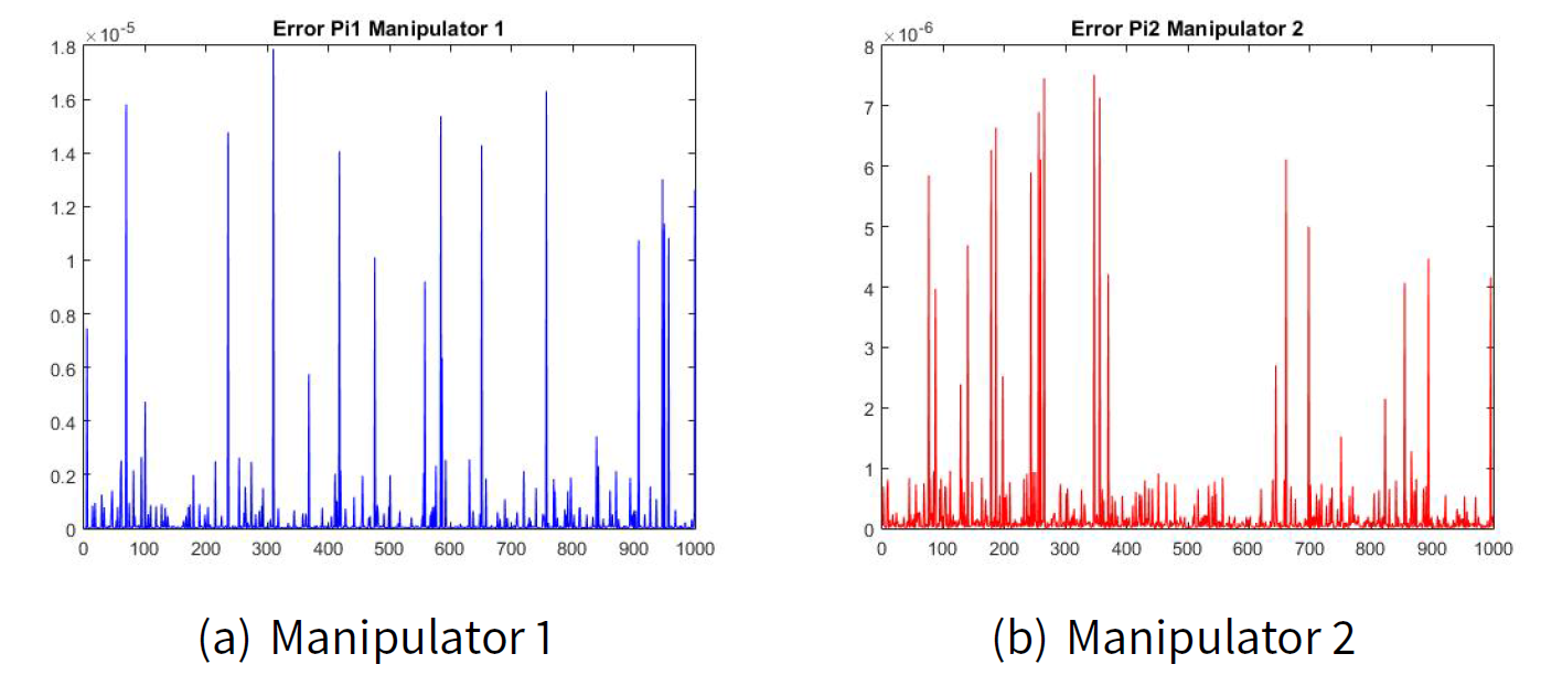
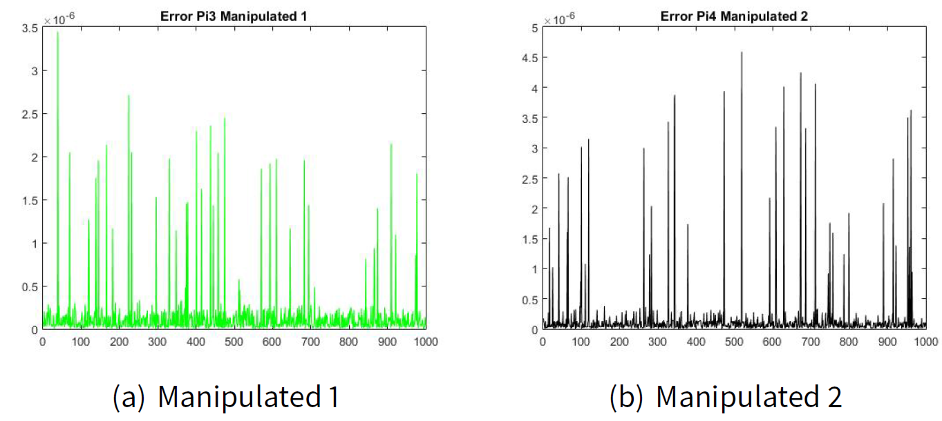
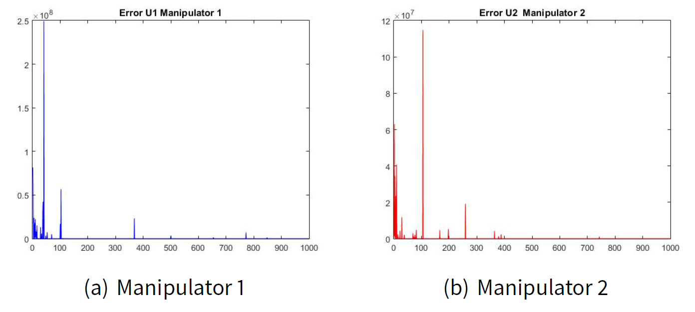
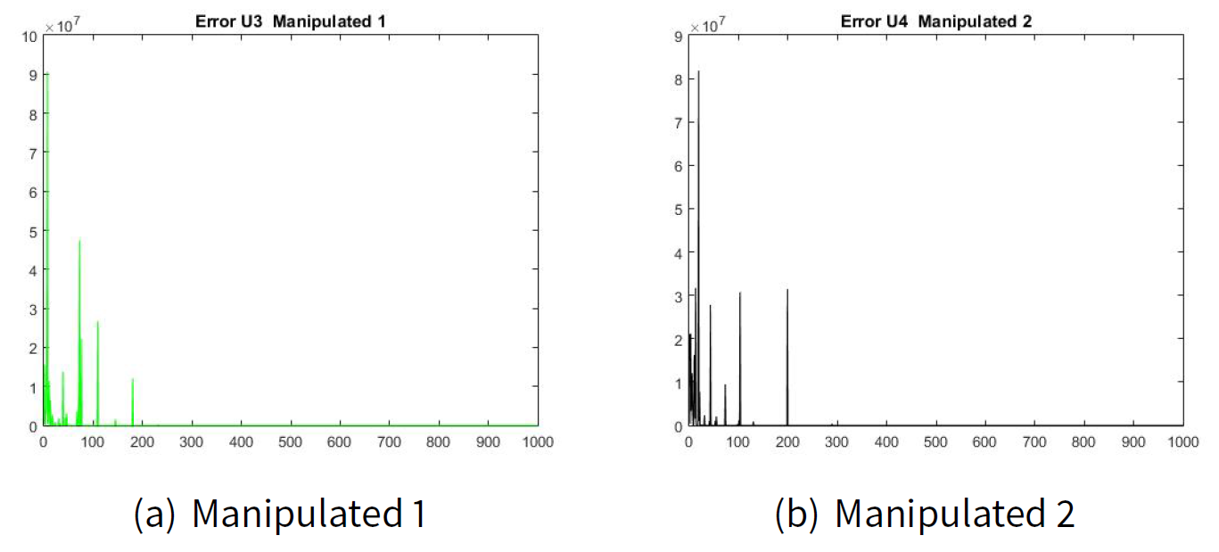
Figures 2(a) and 2(b) show the error of the estimated transition matrix \(\hat{\pi}_{ij|k}\) for the manipulator leader 1 and the error of the estimated transition matrix \(\hat{\pi}_{ij|k}\) for the manipulator leader 2. Figures 3(a) and 2(b) show the error of the estimated transition matrix \(\hat{\pi}_{ij|k}\) for the manipulated follower 1 and the manipulated follower 2. The order of the error e is 1x10⁻⁶ which is very small for our example. As well as, Figures 4 and 5 show the error of the estimated utility \(\hat{J}_{ij|k}\).
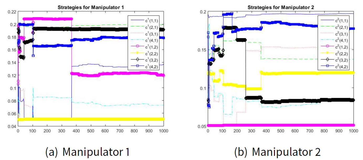
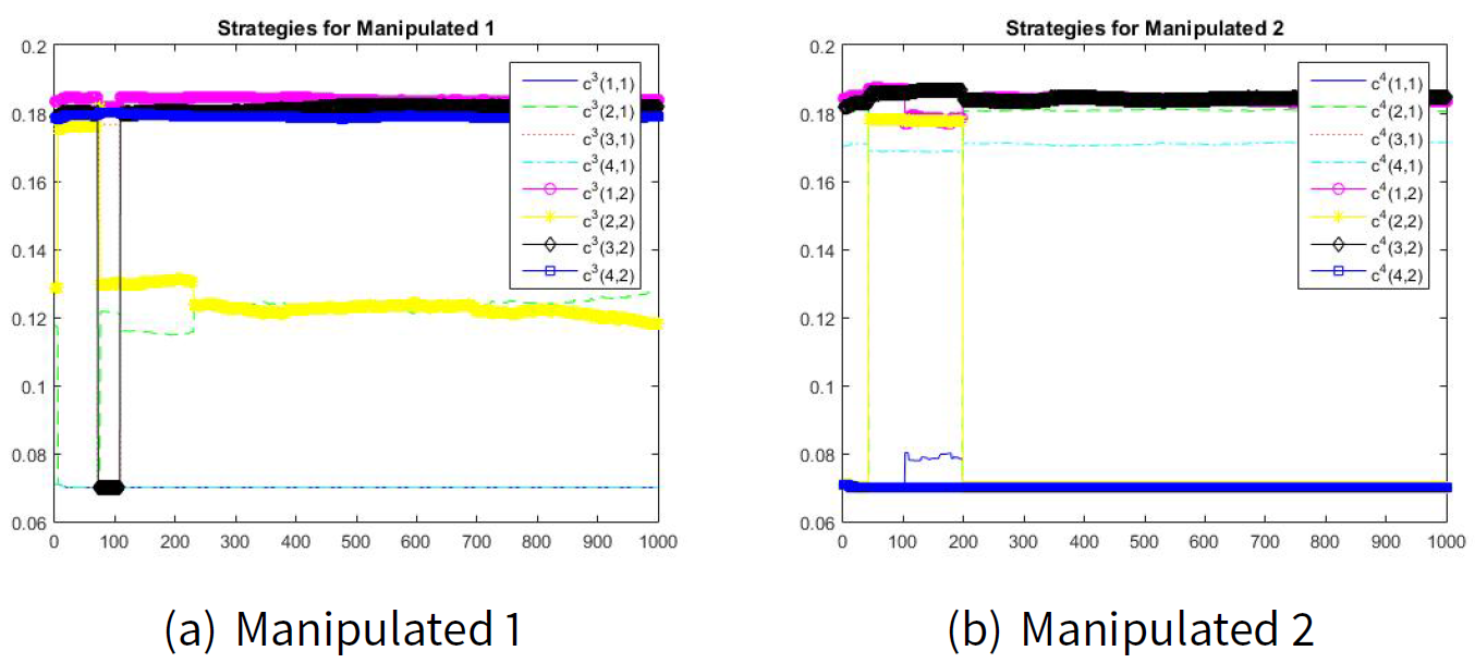
Figures 6 and 7 show the convergence to the manipulation (Machiavellian) equilibrium point. The estimated values for \(\hat{d}_{i|k}\) are as follows:
| $$ \begin{array}{cc} \hat{d}_{i|1k}^{(1)*} \begin{bmatrix} 0.5355 & 0.4645 \\ 0.7965 & 0.2035 \\ 0.2105 & 0.7895 \\ 0.2904 & 0.7096 \end{bmatrix} & \hat{d}_{i|1k}^{(2)*} \begin{bmatrix} 0.7937 & 0.2063 \\ 0.5349 & 0.4651 \\ 0.6431 & 0.3569 \\ 0.3161 & 0.6839 \end{bmatrix} \end{array} $$ |
| $$ \begin{array}{cc} \hat{d}_{i|1k}^{(3)*} \begin{bmatrix} 0.2757 & 0.7243 \\ 0.5183 & 0.4817 \\ 0.2780 & 0.7220 \\ 0.2812 & 0.7188 \end{bmatrix} & \hat{d}_{i|1k}^{(4)*} \begin{bmatrix} 0.2763 & 0.7237 \\ 0.7206 & 0.2794 \\ 0.2749 & 0.7251 \\ 0.7101 & 0.2899 \end{bmatrix} \end{array} $$ |
Conclusions and future work
In this paper we developed a manipulation model where the manipulator players can anticipate the predicted response of the manipulated players. The proposed Machiavellian game theory approach established a system that analyzes and predicts how players behave in strategic situations combining: strategic thinking, best-reply, and mutual consistency (equilibrium). We justified the mutual consistency to predict how players are likely to behave by introducing a reinforcement learning process. In fact, the equilibrium is the result of a strategic thinking, optimization, and equilibration (or learning).
In our proposed model the manipulators players play a Machiavellian strategy first and the manipulated players move sequentially in terms of the actions proposed by the manipulators. In the dynamics of the model the manipulators players consider the best-reply of the manipulated players, and then select the Machiavellian strategy that optimizes their utility, anticipating the responses of the manipulated players. Subsequently, the manipulated players observe the Machiavellian strategy played by the manipulators players and select their best-reply strategy. The Machiavellian behavior described above coincides with a Stackelberg game. Strategies are selected according to the Machiavellian social conduct theory.
We introduced the utilitarian (immoral behavior) and deontological moral theories for modeling the Machiavellian immorality and, we reviewed psychological findings regarding moral decision making. An advantage of the Machiavellianism is that whereas other moral theories provide standards for how we should act, they do not describe how moral judgments and decisions are achieved in practice. We established a relationship between moral and game theory (economic theories) and we suggested that the reinforcement learning theory, with its principle of error-driven adjustment of cost/reward predictions, provided evidences of how players acquire moral (immoral) behavior.
The introduction of the reinforcement learning theory suggested on the one hand, a mechanism by which utilitarian moral value may guide the Machiavellian behavior, as well as, the deontological moral obtain a value for certain moral principles or acts. We noted some minor differences with the common usage of classical reinforcement learning because the control strategy needs to change as the actor computes the game. This need not pose any problems, as long as the actor parameters are updated on a slower time scale. The main advantage of our approach is that it preserves the convergence properties of the extraproximal method. The result of the model is the manipulation equilibrium point. Validity of the proposed method was successfully demonstrated both theoretically and by a simulated numerical example.
There exist a number of challenges left to be addressed for future work. The obvious next step is to incorporate our model into an implemented explanatory system for testing it with real-life scenarios. An interesting technical challenge is that of finding an analytical solution for the manipulation equilibrium point. An additional interesting problem is to associate the manipulation equilibrium point proposed in this paper with the bagaming problem where players should cooperate when non-cooperation leads to Pareto-inefficient results. It will be interested also to examine the problem of the existence of a manipulation equilibrium point under conditions of moral hazard (when one player takes more risks because someone else bears the cost of those risks). These extensions should lead to a more complete account of complex manipulation understanding.
Appendix: Extraproximal
The individual cost-functions of the leaders are defined as follows:
Cost-functions for the leaders| $$ \mathbf{J}^{1}\left( c_{(i_{1},k_{1})}^{(1)},c_{(i_{2},k_{2})}^{(2)}|c_{(i_{3},k_{3})}^{(3)}c_{(i_{4},k_{4})}^{(4)}\right) =\sum\limits_{i_{1},k_{1}}\sum\limits_{i_{2},k_{2}}\sum\limits_{i_{3},k_{3}}\sum\limits_{i_{4},k_{4}}W_{(i_{1},k_{1};i_{2},k_{2};i_{3},k_{3};i_{4},k_{4})}^{(1)}\left( c_{(i_{1},k_{1})}^{(1)}c_{(i_{2},k_{2})}^{(2)}\right) \left( c_{(i_{3},k_{3})}^{(3)}c_{(i_{4},k_{4})}^{(4)}\right) $$ |
| $$ \mathbf{J}^{2}\left( c_{(i_{1},k_{1})}^{(1)},c_{(i_{2},k_{2})}^{(2)}|c_{(i_{3},k_{3})}^{(3)}c_{(i_{4},k_{4})}^{(4)}\right) =\sum\limits_{i_{1},k_{1}}\sum\limits_{i_{2},k_{2}}\sum\limits_{i_{3},k_{3}}\sum\limits_{i_{4},k_{4}}W_{(i_{1},k_{1};i_{2},k_{2};i_{3},k_{3};i_{4},k_{4})}^{(2)}\left( c_{(i_{1},k_{1})}^{(1)}c_{(i_{2},k_{2})}^{(2)}\right) \left( c_{(i_{3},k_{3})}^{(3)}c_{(i_{4},k_{4})}^{(4)}\right) $$ |
| $$ \mathbf{J}^{3}\left( c_{(i_{3},k_{3})}^{(3)}c_{(i_{4},k_{4})}^{(4)}|c_{(i_{1},k_{1})}^{(1)},c_{(i_{2},k_{2})}^{(2)}\right) =\sum\limits_{i_{1},k_{1}}\sum\limits_{i_{2},k_{2}}\sum\limits_{i_{3},k_{3}}\sum\limits_{i_{4},k_{4}}W_{(i_{1},k_{1};i_{2},k_{2};i_{3},k_{3};i_{4},k_{4})}^{(3)}\left( c_{(i_{3},k_{3})}^{(3)}c_{(i_{4},k_{4})}^{(4)}\right) \left( c_{(i_{1},k_{1})}^{(1)}c_{(i_{2},k_{2})}^{(2)}\right) $$ |
| $$ \mathbf{J}^{4}\left( c_{(i_{3},k_{3})}^{(3)}c_{(i_{4},k_{4})}^{(4)}|c_{(i_{1},k_{1})}^{(1)},c_{(i_{2},k_{2})}^{(2)}\right) =\sum\limits_{i_{1},k_{1}}\sum\limits_{i_{2},k_{2}}\sum\limits_{i_{3},k_{3}}\sum\limits_{i_{4},k_{4}}W_{(i_{1},k_{1};i_{2},k_{2};i_{3},k_{3};i_{4},k_{4})}^{(4)}\left( c_{(i_{3},k_{3})}^{(3)}c_{(i_{4},k_{4})}^{(4)}\right) \left( c_{(i_{1},k_{1})}^{(1)}c_{(i_{2},k_{2})}^{(2)}\right) $$ |
Considering that
| $$ \begin{array}{c} \mathbf{J}^{1}\left( \mathring{c}_{(i_{1},k_{1})}^{(1)},c_{(i_{2},k_{2})}^{( \hat{2})}|c_{(i_{3},k_{3})}^{(3)}c_{(i_{4},k_{4})}^{(4)}\right) \leq \mathbf{ J}^{1}\left( c_{(i_{1},k_{1})}^{(1)},c_{(i_{2},k_{2})}^{(\hat{2} )}|c_{(i_{3},k_{3})}^{(3)}c_{(i_{4},k_{4})}^{(4)}\right) \\ \mathbf{J}^{2}\left( c_{(i_{1},k_{1})}^{(\hat{1})},\mathring{c} _{(i_{2},k_{2})}^{(2)}|c_{(i_{3},k_{3})}^{(3)}c_{(i_{4},k_{4})}^{(4)}\right) \leq \mathbf{J}^{2}\left( c_{(i_{1},k_{1})}^{(\hat{1} )},c_{(i_{2},k_{2})}^{(2)}|c_{(i_{3},k_{3})}^{(3)}c_{(i_{4},k_{4})}^{(4)} \right) \end{array} $$ |
| $$ \begin{array}{c} \mathbf{J}^{3}\left( \mathring{c}_{(i_{3},k_{3})}^{(3)}c_{(i_{4},k_{4})}^{( \hat{4})}|c_{(i_{1},k_{1})}^{(1)},c_{(i_{2},k_{2})}^{(2)}\right) \leq \mathbf{J}^{3}\left( c_{(i_{3},k_{3})}^{(3)}c_{(i_{4},k_{4})}^{(\hat{4} )}|c_{(i_{1},k_{1})}^{(1)},c_{(i_{2},k_{2})}^{(2)}\right) \\ \mathbf{J}^{4}\left( c_{(i_{3},k_{3})}^{(\hat{3})}\mathring{c} _{(i_{4},k_{4})}^{(4)}|c_{(i_{1},k_{1})}^{(1)},c_{(i_{2},k_{2})}^{(2)} \right) \leq \mathbf{J}^{4}\left( c_{(i_{3},k_{3})}^{(\hat{3} )}c_{(i_{4},k_{4})}^{(4)}|c_{(i_{1},k_{1})}^{(1)},c_{(i_{2},k_{2})}^{(2)} \right) \end{array} $$ |
We have that for the leaders that
| $$ \begin{array}{c} \sum\limits_{l=1}^{\mathcal{N}}\varphi _{l}(\bar{u}^{l},u^{\hat{l}}|v)= \mathbf{J}^{1}\left( \mathring{c}_{(i_{1},k_{1})}^{(1)},c_{(i_{2},k_{2})}^{( \hat{2})}|c_{(i_{3},k_{3})}^{(3)}c_{(i_{4},k_{4})}^{(4)}\right) +\mathbf{J} ^{2}\left( c_{(i_{1},k_{1})}^{(\hat{1})},\mathring{c} _{(i_{2},k_{2})}^{(2)}|c_{(i_{3},k_{3})}^{(3)}c_{(i_{4},k_{4})}^{(4)}\right) = \\ \sum\limits_{i_{1},k_{1}}\sum\limits_{i_{2},k_{2}}\sum\limits_{i_{3},k_{3}} \sum \limits_{i_{4},k_{4}}W_{(i_{1},k_{1};i_{2},k_{2};i_{3},k_{3};i_{4},k_{4})}^{(1)}\left( \mathring{c}_{(i_{1},k_{1})}^{(1)}c_{(i_{2},k_{2})}^{(\hat{2})}\right) \left( c_{(i_{3},k_{3})}^{(3)}c_{(i_{4},k_{4})}^{(4)}\right) + \\ \sum\limits_{i_{1},k_{1}}\sum\limits_{i_{2},k_{2}}\sum\limits_{i_{3},k_{3}} \sum \limits_{i_{4},k_{4}}W_{(i_{1},k_{1};i_{2},k_{2};i_{3},k_{3};i_{4},k_{4})}^{(2)}\left( c_{(i_{1},k_{1})}^{( \hat{1})}\mathring{c}_{(i_{2},k_{2})}^{(2)}\right) \left( c_{(i_{3},k_{3})}^{(3)}c_{(i_{4},k_{4})}^{(4)}\right) \end{array} $$ |
| $$ \begin{array}{c} \sum\limits_{l=1}^{\mathcal{N}}\varphi _{l}(u^{l},u^{\hat{l}}|v)=\mathbf{J} ^{1}\left( c_{(i_{1},k_{1})}^{(1)},c_{(i_{2},k_{2})}^{(\hat{2} )}|c_{(i_{3},k_{3})}^{(3)}c_{(i_{4},k_{4})}^{(4)}\right) +\mathbf{J} ^{2}\left( c_{(i_{1},k_{1})}^{(\hat{1} )},c_{(i_{2},k_{2})}^{(2)}|c_{(i_{3},k_{3})}^{(3)}c_{(i_{4},k_{4})}^{(4)} \right) = \\ \sum\limits_{i_{1},k_{1}}\sum\limits_{i_{2},k_{2}}\sum\limits_{i_{3},k_{3}} \sum \limits_{i_{4},k_{4}}W_{(i_{1},k_{1};i_{2},k_{2};i_{3},k_{3};i_{4},k_{4})}^{(1)}\left( c_{(i_{1},k_{1})}^{(1)}c_{(i_{2},k_{2})}^{( \hat{2})}\right) \left( c_{(i_{3},k_{3})}^{(3)}c_{(i_{4},k_{4})}^{(4)}\right) + \\ \sum\limits_{i_{1},k_{1}}\sum\limits_{i_{2},k_{2}}\sum\limits_{i_{3},k_{3}} \sum \limits_{i_{4},k_{4}}W_{(i_{1},k_{1};i_{2},k_{2};i_{3},k_{3};i_{4},k_{4})}^{(2)}\left( c_{(i_{1},k_{1})}^{( \hat{1})}c_{(i_{2},k_{2})}^{(2)}\right) \left( c_{(i_{3},k_{3})}^{(3)}c_{(i_{4},k_{4})}^{(4)}\right) \end{array} $$ |
For computing the Nash condition for the leaders we define the function \(g(u,\hat{u}(u)|v)\) as follows
| $$ \begin{array}{c} g_{l}(u^{l},\hat{u}^{l}(u)|v)=\sum\limits_{l=1}^{\mathcal{N}}\varphi _{l}( \bar{u}^{l},u^{\hat{l}}|v)-\varphi _{l}(u^{l},u^{\hat{l}}|v) \\ u_{l}=(\bar{u}^{l},u^{\hat{l}}),\text{ }\hat{u}_{l}(u)=(u^{l},u^{\hat{l}}) \\ g(u,\hat{u}(u)|v)=\sum\limits_{l}g_{l}(u_{l},\hat{u}_{l}(u)|v) \\ u=(u_{1}^{T},...,u_{n}^{T})^{T},\hat{u}_{l}(u)=(\hat{u}_{1}^{\top }(u),..., \hat{u}_{n}^{\top }(u))^{\top } \\ \\ u=\left( \begin{array}{c} \begin{array}{c} col\mbox{ }\left\Vert \mathring{c}_{(i_{1},k_{1})}^{(1)}\right\Vert\\ col\mbox{ }\left\Vert c_{(i_{2},k_{2})}^{(\hat{2})}\right\Vert\\ col\mbox{ }\left\Vert c_{(i_{3},k_{3})}^{(3)}\right\Vert\\ col\mbox{ }\left\Vert c_{(i_{4},k_{4})}^{(4)}\right\Vert \end{array} \\ \begin{array}{c} col\mbox{ }\left\Vert c_{(i_{1},k_{1})}^{(\hat{1})}\right\Vert\\ col\mbox{ }\left\Vert \mathring{c}_{(i_{2},k_{2})}^{(2)}\right\Vert\\ col\mbox{ }\left\Vert c_{(i_{3},k_{3})}^{(3)}\right\Vert\\ col\mbox{ }\left\Vert c_{(i_{4},k_{4})}^{(4)}\right\Vert \end{array} \end{array} \right) ,\hat{u}(u)=\left( \begin{array}{c} \begin{array}{c} col\mbox{ }\left\Vert c_{(i_{1},k_{1})}^{(1)}\right\Vert\\ col\mbox{ }\left\Vert c_{(i_{2},k_{2})}^{(\hat{2})}\right\Vert\\ col\mbox{ }\left\Vert c_{(i_{3},k_{3})}^{(3)}\right\Vert\\ col\mbox{ }\left\Vert c_{(i_{4},k_{4})}^{(4)}\right\Vert \end{array} \\ \begin{array}{c} col\mbox{ }\left\Vert c_{(i_{1},k_{1})}^{(\hat{1})}\right\Vert\\ col\mbox{ }\left\Vert c_{(i_{2},k_{2})}^{(2)}\right\Vert\\ col\mbox{ }\left\Vert c_{(i_{3},k_{3})}^{(3)}\right\Vert\\ col\mbox{ }\left\Vert c_{(i_{4},k_{4})}^{(4)}\right\Vert \end{array} \end{array} \right) \end{array} \label{fung2} $$ |
For \(n=0,1,...\) let define the vectors
| $$ \begin{array}{c} u_{n}=\left( \begin{array}{c} col\mbox{ }c^{(1)}\left( n\right) \\ col\mbox{ }c^{(2)}\left( n\right) \end{array} \right) \\ \\ \hat{u}_{n}(u)=u^{\hat{l}}=\left( \begin{array}{c} col\mbox{ }c^{(\hat{1})}\left( n\right) \\ col\mbox{ }c^{(\hat{2})}\left( n\right) \end{array} \right) \\ \\ \bar{u}^{l}=\left( \begin{array}{c} col\mbox{ }\mathring{c}^{(1)}\left( n\right) \\ col\mbox{ }\mathring{c}^{(2)}\left( n\right) \end{array} \right) =\left( \begin{array}{c} col\mbox{ }\arg \underset{z\in C_{adm}^{(1)}}{\min }\mathbf{J}^{(1)}(z,c^{( \hat{2})}\left( n\right) ,c^{(3)}\left( n\right) ,c^{(4)}\left( n\right) ) \\ col\mbox{ }\arg \underset{z\in C_{adm}^{(2)}}{\min }\mathbf{J}^{(1)}(c^{( \hat{1})}\left( n\right) ,z,c^{(3)}\left( n\right) ,c^{(4)}\left( n\right) ) \end{array} \right) \end{array} $$ |
The regularized problem for \(G\left( u,\hat{u}(u)|v\right)\) is defined as follows
| $$ \begin{array}{c} G_{\delta }\left( u,\hat{u}(u)|v\right) =\sum\limits_{l=1}^{\mathcal{N} }\varphi _{l}\left( \bar{u}^{l},u^{\hat{l}}|v\right) -\varphi _{l}\left( u^{l},u^{\hat{l}}|v\right) = \\ \sum\limits_{i_{1},k_{1}}\sum\limits_{i_{2},k_{2}}\sum\limits_{i_{3},k_{3}} \sum \limits_{i_{4},k_{4}}W_{(i_{1},k_{1};i_{2},k_{2};i_{3},k_{3};i_{4},k_{4})}^{(1)}\left( \mathring{c}_{(i_{1},k_{1})}^{(1)}c_{(i_{2},k_{2})}^{(\hat{2})}\right) \left( c_{(i_{3},k_{3})}^{(3)}c_{(i_{4},k_{4})}^{(4)}\right) + \\ \sum\limits_{i_{1},k_{1}}\sum\limits_{i_{2},k_{2}}\sum\limits_{i_{3},k_{3}} \sum \limits_{i_{4},k_{4}}W_{(i_{1},k_{1};i_{2},k_{2};i_{3},k_{3};i_{4},k_{4})}^{(2)}\left( c_{(i_{1},k_{1})}^{( \hat{1})}\mathring{c}_{(i_{2},k_{2})}^{(2)}\right) \left( c_{(i_{3},k_{3})}^{(3)}c_{(i_{4},k_{4})}^{(4)}\right) - \\ \sum\limits_{i_{1},k_{1}}\sum\limits_{i_{2},k_{2}}\sum\limits_{i_{3},k_{3}} \sum \limits_{i_{4},k_{4}}W_{(i_{1},k_{1};i_{2},k_{2};i_{3},k_{3};i_{4},k_{4})}^{(1)}\left( c_{(i_{1},k_{1})}^{(1)}c_{(i_{2},k_{2})}^{( \hat{2})}\right) \left( c_{(i_{3},k_{3})}^{(3)}c_{(i_{4},k_{4})}^{(4)}\right) - \\ \sum\limits_{i_{1},k_{1}}\sum\limits_{i_{2},k_{2}}\sum\limits_{i_{3},k_{3}} \sum \limits_{i_{4},k_{4}}W_{(i_{1},k_{1};i_{2},k_{2};i_{3},k_{3};i_{4},k_{4})}^{(2)}\left( c_{(i_{1},k_{1})}^{( \hat{1})}c_{(i_{2},k_{2})}^{(2)}\right) \left( c_{(i_{3},k_{3})}^{(3)}c_{(i_{4},k_{4})}^{(4)}\right) + \\ \frac{\delta }{2}\left( \left\Vert \begin{array}{c} c_{(i_{1},k_{1})}^{(1)} \\ c_{(i_{2},k_{2})}^{(2)} \end{array} \right\Vert ^{2}+\left\Vert \begin{array}{c} c_{(i_{1},k_{1})}^{(\hat{1})} \\ c_{(i_{2},k_{2})}^{(\hat{2})} \end{array} \right\Vert ^{2}\right) \end{array} $$ |
and for \(g(u,\hat{u}(u))\) we have
| $$ \begin{array}{c} g_{\delta }(u,\hat{u}(u)|v)= \\ \sum\limits_{i_{1},k_{1}}\sum\limits_{i_{2},k_{2}}\sum\limits_{i_{3},k_{3}} \sum \limits_{i_{4},k_{4}}W_{(i_{1},k_{1};i_{2},k_{2};i_{3},k_{3};i_{4},k_{4})}^{(1)}\left( \mathring{c}_{(i_{1},k_{1})}^{(1)}c_{(i_{2},k_{2})}^{(\hat{2})}\right) \left( c_{(i_{3},k_{3})}^{(3)}c_{(i_{4},k_{4})}^{(4)}\right) + \\ \sum\limits_{i_{1},k_{1}}\sum\limits_{i_{2},k_{2}}\sum\limits_{i_{3},k_{3}} \sum \limits_{i_{4},k_{4}}W_{(i_{1},k_{1};i_{2},k_{2};i_{3},k_{3};i_{4},k_{4})}^{(2)}\left( c_{(i_{1},k_{1})}^{( \hat{1})}\mathring{c}_{(i_{2},k_{2})}^{(2)}\right) \left( c_{(i_{3},k_{3})}^{(3)}c_{(i_{4},k_{4})}^{(4)}\right) - \\ \sum\limits_{i_{1},k_{1}}\sum\limits_{i_{2},k_{2}}\sum\limits_{i_{3},k_{3}} \sum \limits_{i_{4},k_{4}}W_{(i_{1},k_{1};i_{2},k_{2};i_{3},k_{3};i_{4},k_{4})}^{(1)}\left( c_{(i_{1},k_{1})}^{(1)}c_{(i_{2},k_{2})}^{( \hat{2})}\right) \left( c_{(i_{3},k_{3})}^{(3)}c_{(i_{4},k_{4})}^{(4)}\right) - \\ \sum\limits_{i_{1},k_{1}}\sum\limits_{i_{2},k_{2}}\sum\limits_{i_{3},k_{3}} \sum \limits_{i_{4},k_{4}}W_{(i_{1},k_{1};i_{2},k_{2};i_{3},k_{3};i_{4},k_{4})}^{(2)}\left( c_{(i_{1},k_{1})}^{( \hat{1})}c_{(i_{2},k_{2})}^{(2)}\right) \left( c_{(i_{3},k_{3})}^{(3)}c_{(i_{4},k_{4})}^{(4)}\right) + \\ \frac{\delta }{2}\left( \left\Vert \begin{array}{c} c_{(i_{1},k_{1})}^{(1)} \\ c_{(i_{2},k_{2})}^{(2)} \end{array} \right\Vert ^{2}+\left\Vert \begin{array}{c} c_{(i_{1},k_{1})}^{(\hat{1})} \\ c_{(i_{2},k_{2})}^{(\hat{2})} \end{array} \right\Vert ^{2}\right) \end{array} $$ |
Remark 12 We have a similar development for the followers.
Let us apply the Lagrange principle, then we have
| $$ \begin{array}{c} \mathcal{L}_{\delta }(u,{\hat{u}(u)},v,\hat{v}(v),\omega ,\xi ):=\theta G_{L_{p},\delta }\left( u(\lambda ),\hat{u}(u)|v\right) +\omega g_{\delta }\left( u,\hat{u}(u)|v\right) +\xi f_{\delta }(v,\hat{v}(v)|u)-\frac{\delta }{2}\left( \xi ^{2}+\omega ^{2}\right) = \\ (\theta +\omega )\left[ \sum\limits_{i_{1},k_{1}}\sum\limits_{i_{2},k_{2}} \sum\limits_{i_{3},k_{3}}\sum \limits_{i_{4},k_{4}}W_{(i_{1},k_{1};i_{2},k_{2};i_{3},k_{3};i_{4},k_{4})}^{(1)}\left( \mathring{c}_{(i_{1},k_{1})}^{(1)}c_{(i_{2},k_{2})}^{(\hat{2})}\right) \left( c_{(i_{3},k_{3})}^{(3)}c_{(i_{4},k_{4})}^{(4)}\right) +\right. \\ \sum\limits_{i_{1},k_{1}}\sum\limits_{i_{2},k_{2}}\sum\limits_{i_{3},k_{3}} \sum \limits_{i_{4},k_{4}}W_{(i_{1},k_{1};i_{2},k_{2};i_{3},k_{3};i_{4},k_{4})}^{(2)}\left( c_{(i_{1},k_{1})}^{( \hat{1})}\mathring{c}_{(i_{2},k_{2})}^{(2)}\right) \left( c_{(i_{3},k_{3})}^{(3)}c_{(i_{4},k_{4})}^{(4)}\right) - \\ \sum\limits_{i_{1},k_{1}}\sum\limits_{i_{2},k_{2}}\sum\limits_{i_{3},k_{3}} \sum \limits_{i_{4},k_{4}}W_{(i_{1},k_{1};i_{2},k_{2};i_{3},k_{3};i_{4},k_{4})}^{(1)}\left( c_{(i_{1},k_{1})}^{(1)}c_{(i_{2},k_{2})}^{( \hat{2})}\right) \left( c_{(i_{3},k_{3})}^{(3)}c_{(i_{4},k_{4})}^{(4)}\right) - \\ \sum\limits_{i_{1},k_{1}}\sum\limits_{i_{2},k_{2}}\sum\limits_{i_{3},k_{3}} \sum \limits_{i_{4},k_{4}}W_{(i_{1},k_{1};i_{2},k_{2};i_{3},k_{3};i_{4},k_{4})}^{(2)}\left( c_{(i_{1},k_{1})}^{( \hat{1})}c_{(i_{2},k_{2})}^{(2)}\right) \left( c_{(i_{3},k_{3})}^{(3)}c_{(i_{4},k_{4})}^{(4)}\right) + \\ \left. \frac{\delta }{2}\left( \left\Vert \begin{array}{c} c_{(i_{1},k_{1})}^{(1)} \\ c_{(i_{2},k_{2})}^{(2)} \end{array} \right\Vert ^{2}+\left\Vert \begin{array}{c} c_{(i_{1},k_{1})}^{(\hat{1})} \\ c_{(i_{2},k_{2})}^{(\hat{2})} \end{array} \right\Vert ^{2}\right) \right] + \\ \xi \left[ \sum\limits_{i_{1},k_{1}}\sum\limits_{i_{2},k_{2}}\sum \limits_{i_{3},k_{3}}\sum \limits_{i_{4},k_{4}}W_{(i_{1},k_{1};i_{2},k_{2};i_{3},k_{3};i_{4},k_{4})}^{(3)}\left( \mathring{c}_{(i_{3},k_{3})}^{(3)}c_{(i_{4},k_{4})}^{(\hat{4})}\right) \left( c_{(i_{1},k_{1})}^{(1)}c_{(i_{2},k_{2})}^{(2)}\right) +\right. \\ \sum\limits_{i_{1},k_{1}}\sum\limits_{i_{2},k_{2}}\sum\limits_{i_{3},k_{3}} \sum \limits_{i_{4},k_{4}}W_{(i_{1},k_{1};i_{2},k_{2};i_{3},k_{3};i_{4},k_{4})}^{(4)}\left( c_{(i_{3},k_{3})}^{( \hat{3})}\mathring{c}_{(i_{4},k_{4})}^{(4)}\right) \left( c_{(i_{1},k_{1})}^{(1)}c_{(i_{2},k_{2})}^{(2)}\right) - \\ \sum\limits_{i_{1},k_{1}}\sum\limits_{i_{2},k_{2}}\sum\limits_{i_{3},k_{3}} \sum \limits_{i_{4},k_{4}}W_{(i_{1},k_{1};i_{2},k_{2};i_{3},k_{3};i_{4},k_{4})}^{(3)}\left( c_{(i_{3},k_{3})}^{(3)}c_{(i_{4},k_{4})}^{( \hat{4})}\right) \left( c_{(i_{1},k_{1})}^{(1)}c_{(i_{2},k_{2})}^{(2)}\right) - \\ \sum\limits_{i_{1},k_{1}}\sum\limits_{i_{2},k_{2}}\sum\limits_{i_{3},k_{3}} \sum \limits_{i_{4},k_{4}}W_{(i_{1},k_{1};i_{2},k_{2};i_{3},k_{3};i_{4},k_{4})}^{(4)}\left( c_{(i_{3},k_{3})}^{( \hat{3})}c_{(i_{4},k_{4})}^{(4)}\right) \left( c_{(i_{1},k_{1})}^{(1)}c_{(i_{2},k_{2})}^{(2)}\right) - \\ \left. \frac{\delta }{2}\left( \left\Vert \begin{array}{c} c_{(i_{3},k_{3})}^{(3)} \\ c_{(i_{4},k_{4})}^{(4)} \end{array} \right\Vert ^{2}+\left\Vert \begin{array}{c} c_{(i_{3},k_{3})}^{(\hat{3})} \\ c_{(i_{4},k_{4})}^{(\hat{4})} \end{array} \right\Vert ^{2}\right) \right] -\frac{\delta }{2}\left( \xi ^{2}+\omega ^{2}\right) \end{array} $$ |
The general format iterative version \(\left( n=0,1,...\right)\) of the extraproximal method (Antipin 2005, Trejo et al. 2015, 2016) with some fixed admissible initial values (\(u_{0}\in U\), \(\hat{u}_{0}\in U\), \(v_{0}\in V\), \(\hat{v}_{0}\in V\), \({\omega _{0}\geq 0}\), \({\xi _{0}\geq 0}\)) is as follows:
- 1. The first half-step (prediction):
- 2. The second (basic) half-step
$$ {\omega _{n+1}}=\arg \underset{\omega \geq 0}{\min }\left\{ {\tfrac{1}{2} \Vert \omega -\omega _{n}\Vert ^{2}-\gamma \mathcal{L}{_{\delta }}(\bar{u} _{n},}\overline{{\hat{u}}}{_{n}(u),\bar{v}_{n},}\overline{{\hat{v}}}{ _{n}(v),\omega ,\bar{\xi}_{n})}\right\} $$ $$ {\xi _{n+1}}=\arg \underset{{\xi }\geq 0}{\min }\left\{ {\tfrac{1}{2}\Vert \xi -\xi _{n}\Vert ^{2}-\gamma \mathcal{L}{_{\delta }}({\bar{u}_{n},} \overline{{\hat{u}}}{_{n}(u),\bar{v}_{n},}\overline{{\hat{v}}}{_{n}(v),}\bar{ \omega}_{n},\xi )}\right\} $$ $$ u_{n+1}=\arg \underset{u\in U}{\min }\left\{ {\tfrac{1}{2}\Vert u-u_{n}\Vert ^{2}+\gamma \mathcal{L}{_{\delta }}({u,}\overline{{\hat{u}}}{_{n}(u),\bar{v} _{n},}\overline{{\hat{v}}}{_{n}(v),}\bar{\omega}_{n},\bar{\xi}_{n})}\right\} $$ $$ \hat{u}_{n+1}=\arg \underset{\hat{u}\in \hat{U}}{\min }\left\{ {\tfrac{1}{2} \Vert \hat{u}-\hat{u}_{n}\Vert ^{2}+\gamma \mathcal{L}{_{\delta }}({\bar{u} _{n},\hat{u}(u),\bar{v}_{n},}\overline{{\hat{v}}}{_{n}(v),}\bar{\omega}_{n}, \bar{\xi}_{n})}\right\}\label{2-nd} $$ $$ v_{n+1}=\arg \underset{v\in V}{\min }\left\{ {\tfrac{1}{2}\Vert v-v_{n}\Vert ^{2}-\gamma \mathcal{L}{_{\delta }}({\bar{u}_{n},}\overline{{\hat{u}}}{ _{n}(u),v,}\overline{{\hat{v}}}{_{n}(v)},\bar{\omega}_{n},\bar{\xi}_{n})} \right\} $$ $$ \hat{v}_{n+1}=\arg \underset{\hat{v}\in \hat{V}}{\min }\left\{ {\tfrac{1}{2} \Vert \hat{v}-\hat{v}_{n}\Vert ^{2}-\gamma \mathcal{L}{_{\delta }}({\bar{u} _{n},}\overline{{\hat{u}}}{_{n}(u),\bar{v}_{n},\hat{v}(v),}\bar{\omega}_{n}, \bar{\xi}_{n})}\right\} $$ References
ANTIPIN, A. S. (2005). An extraproximal method for solving equilibrium programming problems and games. Computational Mathematics and Mathematical Physics, 45(11), 1893–1914.
BALES, R. E. (1971). Act-utilitarianism: Account of right-making characteristics or decision-making procedures? American Philosophical Quarterly, 8, 257–265.
BYRNE, R. & Whiten, A. (1988). Machiavellianism Intelligence: The Evolution of the Intellect in monkeys apes and Humans. Claredon Press.
CALHOUN, R. P. (1969). Niccoli machiavelli and the 20th century administrator. Academy of Management Journal, 12, 205–212.
CERVANTES, J. A., Rodriguez, L. F., Lopez, S., Ramos, F. & Robles, F. (2011). Autonomous agents and ethical decision-making. Cognitive Computation, 8, 278–296. [doi:10.1007/s12559-015-9362-8]
CHRISTIE, R. & Geis, F. (1970). Studies in Machiavellianism. Academic Press.
CLECKLEY, H. (1976). The Mask of sanity. Mosby, 5th edn.
CLEMPNER, J. B. & Poznyak, A. S. (2014). Simple computing of the customer lifetime value: A fixed local-optimal policy approach. Journal of Systems Science and Systems Engineering, 23(4), 439–459.
DAWKINS, R. (1976). The selfish gene. Oxford University Press.
DAWKINS, R. & Krebs, J. (1978). Animal signals:Information or manipulation. Blackwell.
DEHGHANI, M., Tomai, E., Forbus, K. & Klenk, M. (2008). An integrated reasoning approach to moral decisionmaking. In Proceedings of the Twenty-Third AAAI Conference on Artificial Intelligence, (pp. 1280–1286). Chicago, Illinois, USA.
FALBO, T. (1977). Multidimensional scaling of power strategies. Multidimensional Scaling of power strategies. Journal of Personality and Social Psychology, 35, 537–547.
GABLE, M., Hollon, C. & Dangello, F. (1992). Managerial structuring of work as a moderator of the machiavellianism and job performance relationship. The Journal of Psychology, 126(3), 317–325. [doi:10.1080/00223980.1992.10543366]
GRAMS, W. & Rogers, R. (1990). Power and personality: Effects of machiavellianism, need for approval, and motivation on use of influence tactics. The Journal of General Psychology, 117(1), 71–82.
HARTOG, D. N. D. & Belschak, F. D. (2012). Work engagement and machiavellianism in the ethical leadership process. Journal of Business Ethics, 107, 35–47. [doi:10.1007/s10551-012-1296-4]
HELLRIEGEL, D., Slocum Jr., J. & Woodman, R. (1997). Organizational Behavior. South-Western Educational Publishing.
INDURKHYA, B. & Misztal-Radecka, J. (2016). Incorporating human dimension in autonomous decision-making on moral and ethical issues. In AAAI Spring Symposium Series, (pp. 226–230). Stanford University.
LEARY, M., Knight, R.& Barns, B. (1986). Ethical ideologies of the machiavellian. Personalityand Social Psychology Bulletin, 12, 75–80.
MACHIAVELLI, N. (1952). The Prince. Encyclopedia Brittanica, Inc.
MACHIAVELLI, N. (1965). Discourses in the first ten books of Titus Livius. Duke University Press.
MACHIAVELLI, N. (2001). The Art of War. Da Capo Press.
MUDRACK, P. (1989). Machiavellianism and locus of control: A meta-analytic review. The Journal of Social Psychology, 130(1), 125–126.
POZNYAK, A. S. (2008). Advanced Mathematical tools for Automatic Control Engineers. Deterministic technique, vol. 1. Elsevier, Amsterdam, Oxford.
POZNYAK, A. S., Najim, K. & Gomez-Ramirez., E. (2000). Self-learning control of finite Markov chains. Marcel Dekker, Inc., New York.
PROCIUK, T. J. & Breen, L. J. (1976). Machiavellianism and locus of control. The Journal of Social Psychology, 9, 141–142. [doi:10.1080/00224545.1976.9923379]
RAVEN, B. H. (1993). Machiavellianism and locus of control. The Journal of Social Psychology, 43(4), 227–251.
SÁNCHEZ, E. M., Clempner, J. B. & Poznyak, A. S. (2015). A priori-knowledge/actor-critic reinforcement learning architecture for computing the mean-variance customer portfolio: The case of bank marmarket campaigns. Engineering Applications of Artificial Intelligence, 46, 82–92. [doi:10.1016/j.engappai.2015.08.011]
SCHINDLER, J. (2012). Rethinking the tragedy of the commons: The integration of socio-psychological dispositions. Journal of Artificial Societies and Social Simulation, 15(1), 4: https://www.jasss.org/15/1/4.html.
SMITH, R. (1979). The psychopath in society. Academic Press.
SOLAR, D. & Bruehl, D. (1971). Machiavellianism and locus of control: Two conceptions of interpersonal power. Psychological Reports, 29, 1079–1082.
STACKELRBERG, H. v. (2011). Market Structure and Equilibrium. Springer. [doi:10.1007/978-3-642-12586-7]
TOBLER, P. N., Kalis, A. & Kalenscher, T. (2008). The role of moral utility in decision making: An interdisciplinary framework. Cognitive, Affective,& Behavioral Neuroscience, 8(4), 390–401.
TREJO, K. K., Clempner, J. B. & Poznyak, A. S. (2015). Computing the Stackelberg/Nash equilibria using the extraproximal method: Convergence analysis and implementation details for Markov Chains games. International Journal of Applied Mathematics and Computer Science, 25(2), 337–351. [doi:10.1515/amcs-2015-0026]
TREJO, K. K., Clempner, J. B. & Poznyak, A. S. (2016). An optimal strong equilibirum solution for cooperative multi-leader-follower Stackelberg Markov Chains games. Kibernetika, 52(2), 258–279.
VECCHIO, R. P. & Sussmann, M. (1991). Choice of influence tactics: Individual and organizational determinants.Journal of Organizational Behavior, 12, 73–80. [doi:10.1002/job.4030120107]
VLEEMING, R. (1979). Machiavellianism and locus of control: Two conceptions of interpersonal power. Psychological Reports, 44, 295–310.
WALLACH, W., Franklin, S. & Allen, C. (2010). A conceptual and computational model of moral decision making in human and artificial agents. Topics in Cognitive Science, 2(3), 454–485. [doi:10.1111/j.1756-8765.2010.01095.x]
WIJERMANS, N., Jorna, R., Jager, W., van Vliet, T. & Adang, O. (2013). Cross: Modelling crowd behaviour with social-cognitive agents. Journal of Artificial Societies and Social Simulation, 16(4), 1: https://www.jasss.org/16/4/1.html.
WILSON, D., Near, D. & Miller, R. (1996). Machiavellianism: A synthesis of the evolutionary and psychological literatures. Psychological Bulletin, 119(2), 285–299. [doi:10.1037/0033-2909.119.2.285]
XIANYU, B. (2010). Social preference, incomplete information, and the evolution of ultimatum game in the small world networks: An agent-based approach. Journal of Artificial Societies and Social Simulation, 13(2), 7: https://www.jasss.org/13/2/7.html.
| $$ {\bar{\omega}_{n}}=\arg \underset{\omega \geq 0}{\min }\left\{ {\tfrac{1}{2} \Vert \omega -\omega _{n}\Vert ^{2}-\gamma \mathcal{L}{_{\delta }}(u_{n}, \hat{u}_{n}(u),v_{n},\hat{v}_{n}(v),\omega ,\bar{\xi}_{n})}\right\} $$ |
| $$ {\bar{\xi}_{n}}=\arg \underset{{\xi }\geq 0}{\min }\left\{ {\tfrac{1}{2} \Vert \xi -\xi _{n}\Vert ^{2}-\gamma \mathcal{L}{_{\delta }}(u_{n},\hat{u} _{n}(u),v_{n},\hat{v}_{n}(v),\bar{\omega}_{n},\xi )}\right\} $$ |
| $$ \bar{u}_{n}=\arg \underset{u\in U}{\min }\left\{ {\tfrac{1}{2}\Vert u-u_{n}\Vert ^{2}+\gamma \mathcal{L}{_{\delta }}(u,\hat{u}_{n}(u),v_{n},\hat{ v}_{n}(v),\bar{\omega}_{n},\bar{\xi}_{n})}\right\} $$ |
| $$ \overline{\hat{u}}_{n}=\arg \underset{\hat{u}\in \hat{U}}{\min }\left\{ { \tfrac{1}{2}\Vert \hat{u}-\hat{u}_{n}\Vert ^{2}+\gamma \mathcal{L}{_{\delta } }(u_{n},\hat{u}(u),v_{n},\hat{v}_{n}(v),\bar{\omega}_{n},\bar{\xi}_{n})} \right\}\label{1-st} $$ | (21) |
| $$ \bar{v}_{n}=\arg \underset{v\in V}{\min }\left\{ {\tfrac{1}{2}\Vert v-v_{n}\Vert ^{2}-\gamma \mathcal{L}{_{\delta }}(u_{n},\hat{u}_{n}(u),v,\hat{ v}_{n}(v),\bar{\omega}_{n},\bar{\xi}_{n})}\right\} $$ |
| $$ \overline{\hat{v}}_{n}=\arg \underset{\hat{v}\in \hat{V}}{\min }\left\{ { \tfrac{1}{2}\Vert \hat{v}-\hat{v}_{n}\Vert ^{2}-\gamma \mathcal{L}{_{\delta } }(u_{n},\hat{u}_{n}(u),v_{n},\hat{v}(v),\bar{\omega}_{n},\bar{\xi}_{n})} \right\} $$ |