
Household debt, precautionary motives and macroeconomic dynamics
As extensively discussed in the recent theoretical and empirical literature, household debt played a key role in the Great Recession in all main advanced economies (Barba & Pivetti 2009). Therefore, the monitoring of the buildup in household debt has been drawing a renewed attention, both among policy makers and in the economic profession. Empirical evidence made clear that both high levels and high growth rates of debt imply an increased vulnerability for households’ balance sheets and question its long run sustainability (Perugini et al. 2016). Because of its role in shaping the business cycle, many studies have been pointing out that high levels of private debt may lead to banking crises (Buyukkarabacak & Valev 2010) and influence the stability of the macroeconomic system (Jordá et al. 2013), especially the intensity of recessions and the likelihood of a financial crisis.
The geography of private debt differs across advanced economies; we deem thus worth discussing how it is actually distributed among OECD countries. We start by considering extra-European countries. Empirical analyses on US data as those by Cynamon & Fazzari (2013) and Zinman (2014) show that, between 2000 and 2007, total household debt doubled and the household debt to GDP ratio has four-folded over the post World-War II period. If we consider also other advanced economies, we see that US patterns are shared among OECD countries.
Here, we report an analysis based on OECD time series on the percentage of household debt on net disposable income over a time span that goes from 2000 to 2014. Figure 1 makes evident that, among extra European countries, the higher ratios of debt-to-disposable income have been experienced by Australia and Switzerland. However, the (rising) trend is very similar across the country’s set, except for Japan where the private sector’s gave rise to a deleveraging process which - following a Fisherian spiral - has been depressing the aggregate demand. The deleveraging phase started in 2004 and it was also more pronounced starting from 2009. Japanese households’ balance sheets were strongly damaged, also as a consequence of the 1990s lost decade (Hayashi & Prescott 2002; Ito & Mishkin 2006) and, as emphasized by Koo (2013), as a result, firms have been minimizing their debts rather than maximizing profits, as well as consumers have been worrying mainly about the level of their loans. In order to distinguish this type of recession from ordinary recessions, it is usually referred to as a balance sheet recession.
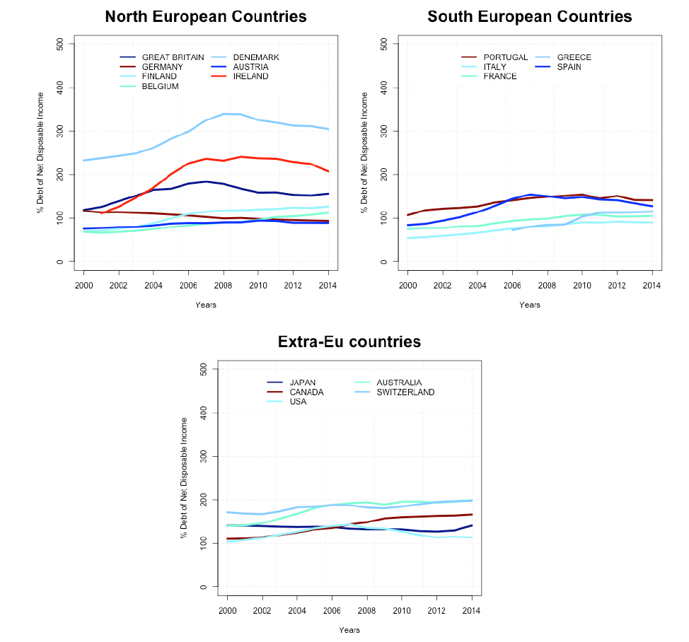
Investigations on household debt in the Euro-Area abound in the recent empirical literature and the overall evidence reports consistent cross-country heterogeneity. Figure 1 shows how high ratios of debt characterize both extra-EU countries as well as the main European economies. Denmark, Great Britain and Ireland display the highest percentage of household debt relative to net disposable income[1]. Considering the period from 2000 to 2014, in Figure 1 we observe that previously to 2007, households’ leverage has grown remarkably in Germany, Italy, Greece and Spain. If we take 2007 as the reference point of the Great Recession’s start, we see as prior to it, debt has been growing steadily in all the considered economies, while in the successive years European households implemented a consistent deleveraging which is especially evident for Greece and Spain. German households began the deleveraging process earlier (in 2004), while Italian households experienced a steadily increasing growth of debt as a percentage of their net disposable income in the time span considered but the ratios are always smaller than those observed in the other countries.
Household debt and macro dynamics: taking a bottom-up approach
Because of the policy concerns raised by the Great Recession, household debt has been drawing a lot of attention by researchers so that the literature on this topic has been blossoming in the last few years. However, several issues are at stake in the investigation of consumption behaviors (Carroll 2012) - and in particular of indebtedness behaviors - in existing mainstream models of consumption. First, many of these models assume representative debtors and creditors, i.e., all households have the same consumption function and the same marginal propensity to consume, which is in contrast with the empirical evidence that marginal propensities to consume differ for people with different financial conditions (wealth, net worth)[2]. In other words, agents’ heterogeneity matters. Second, the budget constraint used in these consumption models implies a borrowing limit, i.e., the consumption problem is solved in face of a budget constraint which prevents households “to die in debt”. This seems an inadequate representation of the consumer problem which flies in the face of reality; indeed, violations of the constraint and illiquid positions or bankruptcy are often observed in the real world. Third, they usually assume a flow of funds from lenders to borrowers within the same sector, namely the private sector (as e.g. Eggertsson & Krugman 2012), but this flow is not intermediated by a banking sector. Moreover, it is usually assumed that consumers are optimizing agents who know exactly how to solve their dynamic programming consumption problem, even in presence of an idiosyncratic shock to their income stream. The optimal solution (consumption level and debt level) is thus always reached because expectations about the future values are always fulfilled.
Recently, many Agent-Based Models (ABM) have investigated the role played by consumption and in particular by household debt. Among the firsts in considering household indebtedness, Erlingsson et al. (2013) focused on the housing market and integrated it into a larger agent-based artificial economy. The model was characterized by four types of agents: workers, firms, banks and a central bank, which interacted through different types of markets: a consumption goods market, a labor market, a housing market and a credit market. They modelled a wealth effect of housing wealth into workers consumption budget as the main link between the housing market and the real economy. Banks extended mortgages to workers only if the expenditure on housing, as a proportion of total income, was lower than a given threshold.
Konig & Grossl (2014) explicitly focused on consumption credit in a framework in which desired consumption was driven by workers disposable income as well as a social norm of consumption, namely the so-called “catch up with the Joneses”, a behavior that reflects a willingness to take on loans. Results showed that varying the strength of the social orientation and prevailing credit constraints, the evolution of macroeconomic time series was largely affected by the “Joneses effect”, while credit constraints determined their volatility.
Seppecher & Salle (2015) built a stock-flow consistent ABM populated by heterogeneous agents. The focus here was on the role played by animal spirits, which propagate the market sentiment (optimism or pessimism) through a contagion model (feedback effect). Agents adapted their financial behavior to their market sentiment, thus influencing the aggregate dynamics and leading to alternating periods of stability and downturns.
Russo et al. (2016) investigated the causal link between increasing inequality and consumer credit in a complex macroeconomic system with financially fragile heterogeneous households, firms and banks. They focused on consumer credit and studied its aggregate effects with particular attention to unsustainable debt levels and the emergence of financial crises. Results showed a mixed support for the increase of household debt as beneficial for the systemic level. On the one hand, the greater availability of credit on the household side boosted aggregate demand; on the other hand, it could progressively lead to a crisis.
Finally, Cardaci & Saraceno (2015) developed a macro stock-flow consistent ABM to study how economic crises emerge in the presence of different credit conditions and income inequality. In particular, they showed how different institutional settings and levels of financialization affect the dynamics of an economy where income inequality plays a role. They discussed the implications of rising household debt and of a policy aimed at tackling inequality by means of a more progressive tax system. Their results showed that fiscal policies can compensate for the rise in income disparities and therefore stabilize the economy.
Taking a bottom up approach, our paper develops an agent-based model populated by heterogeneous consumers, a production sector and a banking sector. The model investigates the complex relationship that emerges from the interaction of the three sectors in a stylized labor market, a credit market and a goods market. The main features of the model can be summarized as follows:
- it stresses the role played by beliefs formed by backward-looking households on future macroeconomic conditions;
- it emphasizes the role of expectations in the production decision: the production sector is considered as bounded rational and endowed with a mechanism to forecast the demand it will receive from the household sector;
- it accounts for different labor market matching mechanisms which contribute to the aggregate performance of the model.
In particular, considering belief and expectations in our model is especially relevant because they allow us to account for more realistic features of human behaviors (Simon 1955). This modeling choice rests on the critique developed by Muth (1961) about the unsoundness of the rational expectation hypothesis (REH), which assumed away any forecasting error possibly made by economic agents. Following Kirman (2014), the main objections to rational expectations fall in four classes: logical or philosophical, econometric or statistical, empirical and experimental evidence. In the last 20 years, theoretical models of heterogeneous bounded rational agents (HAM) (Hommes 2006) and agent-based financial models have literally blossomed. Starting from the seminal contribution of Brock & Hommes (1997), many researchers have engaged in the building of “heuristics switching models”. In those models agents have a set of simple forecasting heuristics (adaptive, trend extrapolating and so on) and choose those that had a better past performance. Hommes (2007, 2011) explore the behavioral space of the heterogeneous expectations hypothesis. By combining the experimental method and evolutionary techniques, Hommes (2007) provided evidence for the importance of heterogeneity in a theory of expectations: by means of a simple heuristics switching model it is possible to fit different behaviors collected from learning to forecast experiments. These results are indeed crucial for economic theory in that they clearly demonstrate that the rational expectation hypothesis occurs only in stable markets (Hommes 2011).
Our model shares with the models described above the acknowledgment that economic agents have different expectations so that working with a rational representative agents is reductive and can lead to misleading results (Kirman 1992). By considering heterogeneous consumers we are able to overcome the so-called Aristotelian fallacy of division[3] as well as the fallacy of composition[4]. Regarding the way in which the expectations are formed, we consider a bounded rational mechanism according to which consumers are backward-looking. In particular, we do not assume mathematical expectations; we rather define them beliefs. The bounded rational behavior of consumers implies that they look at their past employment or unemployment states and form beliefs over future states of the economy accordingly.
The focus of our investigation is primarily on the link among unemployment and individual willingness to borrow and to the extent to which their interaction contributes to the aggregate dynamics of the artificial economy. Nevertheless, we take a different perspective with respect to other ABM that deal with household debt because the micro level of our model tends to emphasize the role of precautionary motives. Our choice is motivated by the emphasis, both theoretical and empirical, on the role played by precautionary motives over the business cycle (Skinner 1988; Carroll 1992; Gourinchas & Parker 2001; Challe & Ragot 2016) and because they can explain a large fraction of individual and aggregate wealth accumulation (see Carroll et al. 2014b; LeBlanc et al. 2015, among others)[5].
Moreover, we think that observing precautionary motives becomes especially relevant when consumers face borrowing constraints (as during economic downturns). Indeed, because of the existence of a link between precautionary motives and imperfections in financial markets, we decided to study the aggregate dynamics of consumers’ behaviors in an agent-based economy that has allowed us to “externalize” the so-called natural borrowing constraint[6]. In this way, we are able to account for agents’ heterogeneity and to consider consumers’ willingness to borrow that strongly depends on macroeconomic conditions.
The rest of the paper is organized as follows. Section 2 presents an overview of the model and the different sectors it is composed of. We provide detailed behavioral equations at the micro level for the household sector, while, for the sake of tractability, the other sectors are treated as aggregates. Section 3 describes how we implement the model in an agent-based setting, the sequence of events and the baseline parametrization. The section is organized in three subsections. The first subsection presents the baseline parameters and their setting. The second subsection reports and discusses the main results gathered from simulations run over the baseline parametrization. The third subsection describes the comparison between artificial and empirical wealth distributions and discusses some sensitivity analyses we perform over the labor market matching mechanisms. Section 4 provides concluding remarks.
The model
The model is composed of an household sector, a production sector and a banking sector. The household sector is made up of heterogeneous agents which are workers and consumers at the same time. They interact with the banking sector and the production sector, which are both treated as a whole.
Before describing the details of the model, is worth emphasizing that it has been mainly motivated by the aim to investigate the role of households financial position over changing macroeconomic conditions. The purpose of the model is indeed to build a minimal framework in order to study this specific phenomenon, leaving aside at this stage of the research other major issues and modeling details related to the other sectors of the macro setting. It can thus be thought of as a partial model in which the aspects that are not explicitly focused on end up in an hidden black box that represent the complement of the analyzed part of the economy. Therefore, several issues such as the destination of the production sector’s profits (outflow), the financing of the unemployment dole (inflow) and many other flow variables are thus not treated in a partial model. The results presented and discussed in the paper depend thus mainly on the combination of parameters as described in Tables 1 and 2. Our strategy is to explore the parameters’ space in order to exclude those regions that lead to unreasonable results for the agents included in the observed part of the economy. Sensitivity analyses, which consist in changing one parameter at a time, allow an accurate evaluation of the model aggregate behavior in the selected part of the parameters’ space. The extension of the model in order to include more sophisticated mechanisms in all the main sectors of the economy is an ambitious goal for future research.
The following paragraph presents the sequence of events performed at each time step by the ABM that implements the model.
Sequence of events
The artificial economy is considered as a discrete iterative system where agents repeat the same set of actions at each time step.
- the Production sector sets production and demands production factors;
- the Labor market opens;
- Consumers receive either wages (if employed) or dole (if unemployed);
- the Production sector makes the production according to the factors obtained in the market;
- the Bank computes interests and asks for loan repayment to indebted consumers;
- Consumers refund if they have enough financial resources; otherwise they are labeled as in “financial difficulty”;
- the Bank updates its balance sheet;
- Consumers form beliefs by looking at the rate of unemployment and set their desired consumption; if it is higher than financial resources, the consumer asks for credit;
- the Credit market opens;
- the Bank decides how much credit to extend;
- the Bank computes the sum of credit demanded and the new credit it can offer; credit requests are either fulfilled or rationed;
- Consumers who asked for credit set their effective consumption according to the obtained credit;
- the Goods market opens: the production sector sells the produced items to households (supply is constrained by production capacity);
- Consumers update their financial position;
- the Production sector computes the economic result.
In the following subsection, we present in details the microeconomics of the three actors that compose our model.
Households
Each household:
- receives either a wage (if employed) from the firm or a dole (if unemployed);
- has a minimum consumption level, \(\bar{c}\) (which is assumed to take the same value as the unemployment dole);
- may ask for loans.
Household’s \(h\) wealth at time \(t\) is denoted by \(W_{h,t}\)and it is equal to the household’s bank account, being other stores of value absent in this model. The wealth level significantly affects the possibility to consume: if a household obtained credit in the past (\(W_{h,t}<0\)), the bank asks her/him to payback the sum of interests (\(i_L\) is the interest rate on borrowing) and the installment (\(\theta\) is the share of principal to be refunded), namely
| $$payback_{h,t} = i_LW_{h,t} + \theta W_{h,t}.$$ | (1) |
In this model, a household’s consumption level cannot be lower than the subsistence level; the payback is thus delayed for households in financial difficulty. Households in good economic conditions (employed or unemployed having a positive bank account) evaluate the possibility to consume more than the subsistence level.
They first compute the desired consumption as follows:
| $$c^d_{h,t}=\max\left(\frac{1+\rho_{h,t}}{1+i_L} y^A_{h,t}+ \beta \max(W_{h,t},0),\bar{c}\right) $$ | (2) |
| $$y^A_{h,t} = wage_{h,t} + payback_{h,t}$$ |
\(\rho_{h,t}\) is a “behavioral” parameter describing individual household’s beliefs. It is computed using the following logistic function (more details are given in next subsections):
| $$\rho_{h,t}(x_{h,t}) = \frac{2}{1+\exp(-\tau_h(x_{h,t}-\hat{x}_h))}-1+i_L \quad \text{with} \quad x_{h,t} = \sum_{j=1}^{m_h} E_{h,t-j}$$ | (3) |
Beliefs and consumption behaviors
Equation (3) states that household’s beliefs depend on the employment record. Households’ sensitivity to the employment record is controlled by the parameter \(\tau_h\): the higher \(\tau_h\), the more consumers respond to changes in \(x_{h,t}\). Note that \(x_{h,t}\in\{0,1,\cdots,m_h\}\). Consider an indebted household. Because \(\rho_{h,t}(0)< i_L<\rho_{h,t}(m_{h})\), s/he can switch from asking for additional credit to saving or vice versa according to his past employment experience and behavioral features. In particular, equations (3) and (2) imply that s/he will ask for additional credit if \(x_{h,t}>\hat{x}_h\) and will save (reducing her/his debt) in the opposite case. It follows that \(\hat{x}_h\) is a crucial parameter: the higher \(\hat{x}_h\), the lower credit demands will be. Consider for example a household with \(\hat{x}_h=m_h\). In this case, s/he is very prudent because he will never borrow; at most he will consume all the available income if s/he was always employed in the latest \(m_h\) periods.
Below we will focus in particular on the \(\hat{x}_h\) parameter. It is thus convenient to gain a fine tuning control on its setting. To this aim, we use a beta distribution \(\mathcal{B}(s_1,s_2)\):
| $$\hat{x}_h= \hat{x}_{\min}+\mathcal{B}(s_1,s_2)(\hat{x}_{\max}-\hat{x}_{\min})$$ | (4) |
In particular, we will analyze the effects of changing the \(s_1\) shape parameter while the second shape parameter is kept constant at 1. As it is known, \(\mathcal{B}(1,1)\) is a uniform distribution. One can cumulate density on the higher values of the distribution by increasing \(s_1\).
Summing up, \(\rho_{h,t}\)affects the slope of the consumption function. Consider indebted consumers:
- those who have \(\frac{1+\rho_{h,t}}{1+i}<1\) are able to consume the desired levels, thus effective consumption \(c_{h,t}\) equals desired consumption \(c_{h,t}=c^d_{h,t}\) and they have a positive cash flow (saving);
- \(\frac{1+\rho_{h,t}}{1+i}>1\) implies \(c^d_{h,t}>y^A_{h,t}\). These consumers ask for new loans to the bank to meet their desired consumption levels.
By “externalizing” the borrowing constraint (compared to the so-called natural borrowing constraint as discussed in Carroll et al. 2012), i.e., by explicitly considering a banking sector that decides whether to provide credit to consumers, households are not able to correctly anticipate the credit rationing possibly implemented by the bank. This has important implications for their consumption decisions (micro level) and for the aggregate consumption function.
Credit demand
According to (2), new credit is demanded in two occurrences:
- households with positive wealth, whose desired consumption is higher than the sum of income and wealth. In this case, new demanded credit is:
$$\Delta L^d_{h,t}=c^d_{h,t}-wage_{h,t}-W_{h,t}(1+i_D)$$ (5) - households with negative wealth, whose income ensures the subsistence consumption level and the bank repayment. In this case new demanded credit is:
| $$\Delta L^d_{h,t}=c^d_{h,t}-[wage_{h,t}+(i_L+\theta)W_{h,t}] $$ | (6) |
If \(y^A_{h,t} < \bar{c}\), we say the household has financial difficulties and the payback is delayed.
The production sector
In this version of the model, we do not consider a multiplicity of firms, rather we decide to model the production sector as a whole. It produces non-durable perishable consumption goods that are not previously ordered by households. Therefore, production is carried out in advance with respect to the demand by households and inventories cannot be carried over to the next period.
In this setting, forecasting the future level of demand as precisely as possible is a crucial task for the entrepreneur. On the same line, for example, Mandel et al. (2010), endow the production sector with an extrapolation methods (i.e., the Winter-Holt forecasting), so that firms forecast future sales and households future income. In their model, expectations updating takes place every period. By means of exponential smoothing, firms update their sales expectations, they thus update their target production and decide of future investments in fixed capital.
A similar mechanism has been implemented by Assenza et al. (2015). In their model, at the beginning of each time step each firm set its selling price and its current production. At the end of each period, firms learn also the average price. Once production has been carried out and search and matching has taken place, each firm can observe the amount of consumption goods actually sold. Since sales occur only after the firm has carried out production, actual demand can differ from current production, this implies a positive/negative forecasting error.
The production process in our model has similarities with that adopted in the cited literature. The production sector performs the following activities:
- decides the level of production;
- demands the production factors needed to make the production;
- makes the production according to the factors obtained on the markets;
- sells the produced items to households who demand for them;
- computes the economic result.
We explain them in more details in the following sections.
Deciding the level of production
We depart from the existing literature by developing a method to forecast the next period demand. The production sector decides the production \(\hat{Y}_t\) extrapolating a value from the trend of past production levels. In particular, a linear and nonlinear fit of the latest \(F\) levels of demand are performed. The best performing between the two models is chosen by comparing their sum of squared errors (\(SSE\)) and it is then used to extrapolate the demand trend. We use the ordinary least square regression on the \(F\) observations as a linear model.
The nonlinear fit is obtained smoothing a wider window of demand values by the LOESS non parametric technique (Cleveland et al. 1992). As it is well known, a non parametric fit crucially depends on the bandwidth used; we develop a procedure to choose this parameter. Our procedure requires that the final part of the fitting line (i.e. the latest \(F\) points) is concave or convex. In other words, we choose the lowest bandwidth which implies the same sign for all the second differences of the latest \(F\) fitted values. Once the bandwidth is selected, we compute the \(SSE\) of the latest \(F\) observations for comparison with the \(SSE\) obtained with the linear model.
If we observe a lower \(SSE\) for the linear model, the regression line is used to obtain the demand forecast, \(\hat{Y}_t\); otherwise, we obtain a parametric version of the final part of the non parametric fitting line by computing the Lagrange interpolation polynomial on the latest \(F\) fitted values. We then use the Lagrange polynomial to obtain \(\hat{Y}\).
Making production
For the sake of simplicity, production in our economy requires only labor as an input. We use the following production function:
| $$Y_t=\sum_{h=1}^{H} \psi_hE_{h,t}$$ | (7) |
Therefore, to realize the production \(\hat{Y}_t\), workers are hired until the sum of their productivities allows to obtain a level of production sufficient to satisfy the expected demand:
| $$Y_t \ge \hat{Y}_t.$$ |
In this setting, the production sector’s problem is thus to set households’ employment states at each time, i.e. to identify the dynamics of \(\mathbf{E}:=\{E_1,E_2,\dots,E_H\}\).
A simple and intuitive way to proceed in our heterogeneous productivity system is to sort individual productivities in a decreasing order and let the production sector hiring at each time step, starting ^from the first ranked until \(Y \ge \hat{Y}\). However, this mechanism implies that the most productive workers are always employed as well as the less productive are always unemployed, therefore the turnover will involve a limited number of workers. Furthermore, this mechanism would pose problems if homogeneous productivities would be considered.
We thus propose an implementation of a hiring mechanism that enlivens the workers’ turnover and that will work well also for a degenerate productivity distributions. The main idea at the core of this implementation is that each household sends a signal about its productivity to the production sector. However, because of market imperfections, signals perceived by the production sector can be different from those sent:
| $$\text{worker sends } \psi_h \qquad \rightarrow \qquad \text{production sector receives } \phi_h$$ |
Technically, we model this communication process as follows:
| $$\phi_{h,t}=SP \times \psi_h+SR \times u_{h,t} $$ | (8) |
Different market labor dynamics are obtained as follows. At each time step, all the households’ employment states are set to 0 before the hiring process is started. Each household sends her/his signal (\(\psi_{h}\)) to the production sector. New values for the employment states are assigned by sorting the perceived signals \(\phi_{h,t}\) in decreasing order i.e. the production sector, starts from the top and continues hiring until
| $$Y_t \ge \hat{Y}_t.$$ |
According to this modeling choice, a static labor market where the most productive workers always get a job can be obtained by setting \(SP>0\) and \(SR=0\). On the other hand, high values of \(SR\) denote lively households’ employment states dynamics.
As will be explained below, this dynamics is our model’s main determinant of households’ consumption.
Economic result
The production sector costs are given by wages. Provided that a worker was hired, his wage is
| $$w_h=w_{\min}+\xi \psi_h$$ | (9) |
The total wage to be payed is thus
| $$WB_t=\sum_{h=1}^{H}w_hE_{h,t}$$ |
In our model, revenue from sales are collected at the end of the production cycle while workers must be paid during production. This creates an important role for credit: the production sector asks for loans to pay wages:
| $$L^d_{f,t}=WB_t.$$ |
Revenues comes from sales and are equal to the obtained demand \(DH_t\). Part of them are used to refund the bank, therefore, the economic result from the entrepreneurial activity is
| $$\pi_t=DH_t-WB_t$$ |
The banking sector
For the sake of simplicity, a representative commercial bank is considered. According to what has been explained in the previous section, some households deposit money at the bank (income after consumption), while others demand credit according to their desired consumption levels and the resulting cash flow gaps. The banking sector also lends to the production sector that asks credit to pay wages.
The bank balance sheet in this model is \(L^H_{t}+L^F_t=D_t+A_t\), where \(L^H_{t}\) is total credit to all household, \(L^F_t\) is credit to the production sector, \(D_t\) deposits from households and \(A_t\) is bank’s equity. Because the focus of the model presented in this paper is on households, we let the banking sector extend to the production sector all the asked credit (\(L^F_t=L^d_{f,t}\)), while we will model explicitly the banking sector balance sheet items which are affected by households’ behavior: \(L^H_{t}\) and \(D_t\).
At each time, households can be divided in two groups: the set of those having a positive wealth \(H^+_{W,t}\), and the set of those with negative wealth \(H^-_{W,t}\), so that we have:
| $$ D_t=\sum_{h \in H^+_{W,t}}W_{h,t} \quad \text{and} \quad L^H_{t}=\sum_{h\in H^-_{W,t}}W_{h,t}.$$ |
It is assumed that the bank uses the following rule for limiting \(L^H\):
| $$L^H_{t}<\lambda D_t.$$ | (10) |
| $$\Delta {L^H_{t}}^s = \max(\lambda D_t-L^H_{t-1},0) \qquad \text{and} \qquad \Delta {L^H_{t}}^d =\sum_h \Delta L^d_{h,t}.$$ |
| $$r_t=\frac{\Delta {L^H_{t}}^d-\Delta {L^H_{t}}^s}{\Delta {L^H_{t}}^d} \qquad\text{note that} \ 0\le r_t \le 1.$$ |
| $$\Delta L^H_{t}=\Delta {L^H_{t}}^d(1-r_t) \qquad \text{and} \qquad \Delta L_{h,t}=\Delta L^d_{h,t}(1-r_t).$$ |
Simulations
Parametrization
Tables 1 and 2 report the baseline parameters values used in simulations[9]. In particular, the parameters in Table 1 are single instances, i.e. they are valid for the whole system and their values are used in computations performed by all agents. Parameters reported in Table 2 regulate households’ heterogeneity and are set in term of statistical distributions. Differently from the single instance parameters, their values differ among agents.
| Parameter | Description | Value | in equation(s) |
|---|---|---|---|
| H | Number of agents | 1000 | |
| SP | signal productivity | 1 | (8) |
| SR | signal randomness | 0.5 | (8) |
| propensity to consume out of wealth | 0.2 | (2) | |
| c | minimum consumption | 45 | (2) |
| d | unemployment dole | 46 | |
| \(w_{min}\) | minimum wage | 46 | (9) |
| wage slope | 0.25 | (9) | |
| iL | monthly interest rate on loans | 0.003 | (1),(6) |
| iD | monthly interest rate on deposits | 0.001 | (5) |
| monthly installment share | 0.01 | (1),(6) | |
| bank LH /DH target | 0.5 | (10) |
Baseline scenario: simulation results
We investigated the micro and macro properties of the model described in the previous section through extensive computer simulations. Hereby, we report the simulation analysis of the model in two steps. In the first one, we give an overall description of the dynamics generated by the model, while in the second one we focus on the effects of different features of the labor market.
| Parameter | Description | Distribution | in equation(s) |
| \(m_h\) | agent’s memory length | Uniform | (3) |
| mean=5 | |||
| variance=0 | |||
| \(\tau_h\) | \(\rho\) slope | Uniform | (3) |
| mean=0.5 | |||
| variance=0 | |||
| \(\hat{x}\) | \(\rho\) location | Beta \(\mathcal{B}(s_1,s_2)\) | (3),(4) |
| \(s_1^{\min}\)=1 | |||
| \(s_1^{\max}\)=100 | |||
| \(s_2\)=1 | |||
| \(\hat{x}_{\min}\)=1 | |||
| \(\hat{x}_{\max}\)=100 | |||
| \(\psi_{h}\) | workers’ productivity | Pareto \(\mathcal{P}(p_1,p_2)\) | (7),(8) |
| slope \(p_1\) = 100 | |||
| position \(p_2\) = 74.25 |
To gain a global knowledge of the model output, starting from the next, we present the effects of changing one at a time the parameters governing a particular aspect of the model. Remarkable attention is given to the effects of changing the consumers’ willingness to borrow attitude (\(s_1\) parameter). Because this parameter plays a crucial role in our model, we report detailed results and sensitivity analysis for three values of this parameter. We choose a low, medium and high value because they grasp the variety of results generated by the model. We then focus our attention on the effects of the different \(s_1\) parametrizations on the wealth distribution. In this respect, we are interested in assessing whether data gathered from our simulations have similarities with the empirical wealth distributions computed from the HFCS (European Household Finance and Consumption Survey) data set to perform an ex-post validation[10] of our agent-based model (Klügl 2008). We report our analysis starting from paragraph 3.21.
The main aim of this section is to monitor the evolution of the real (employment and consumption) and financial (deposits, loans and wealth) variables in the baseline parametrization.
Figure 2 offers a global overview of the model outcomes with special attention to the health of the banking sector, the employment level and its fluctuations. It shows average values of these variables for different shapes of the willingness to borrows distribution (different levels of \(s_1\)) and unemployment dole (\(d\)).
Figure 2A reports three lines for each level of the unemployment dole. They are the minimum, the average and the maximum number of employees observed in each run. The chart allows us to assess the average performance of the economy as well as of the volatility observed over different parametrizations. Looking at the average values, we can see how an increase in the dole implies a higher employment level. The shape of the willingness to borrow distribution (\(s_1\)) does not affect significantly the average employment level, but it impacts on its fluctuations: the employment range decreases for low values of \(s_1\), but then it increases as \(s_1\) becomes higher. An exception is detected when the dole is equal to the subsistence level of consumption (\(\bar{c}=45\)). In this case, fluctuations amplitude are constant when \(s_1\) increases (see the black lines in Figure 2A). The progressive increase of the dole speeds up the appearance of fluctuations whose amplitude increase faster with \(s_1\) for higher levels of the dole. By looking at Figure 2A, we can observe that blue lines (\(d=48\)) show a dynamics that precedes the green lines (\(d=47\)) which in turn precede the red lines (\(d=46\)).
Figures 2B and 2C aim at highlighting particular aspects of the labor market whose deduction from Figure 2A could be hampered by the several lines included in the plot. In particular, Figure 2B reports the highest level of the unemployment rate observed in simulations for each combination (\(d\); \(s_1\)), while Figure 2C display the difference between the highest and the lowest unemployment rate observed in the same simulations. When the dole is equal to the subsistence level of consumption (\(d=\bar{c}=45\)), the maximum unemployment rate decreases when s1 goes from 1 to about 15 and roughly keeps constant for higher level of \(s_1\) (black line in Figure 2B). The gap between the maximum and the minimum unemployment rate has a similar pattern and fluctuates around a value slightly below 5% for \(s_1>15\) (black line in Figure 2C). Both the maximum unemployment and the gap between the maximum and minimum unemployment rate approach a level close to 35% for higher levels of the dole although this happens at different speeds as highlighted above (see the coloured lines in Figures 2B and 2C).
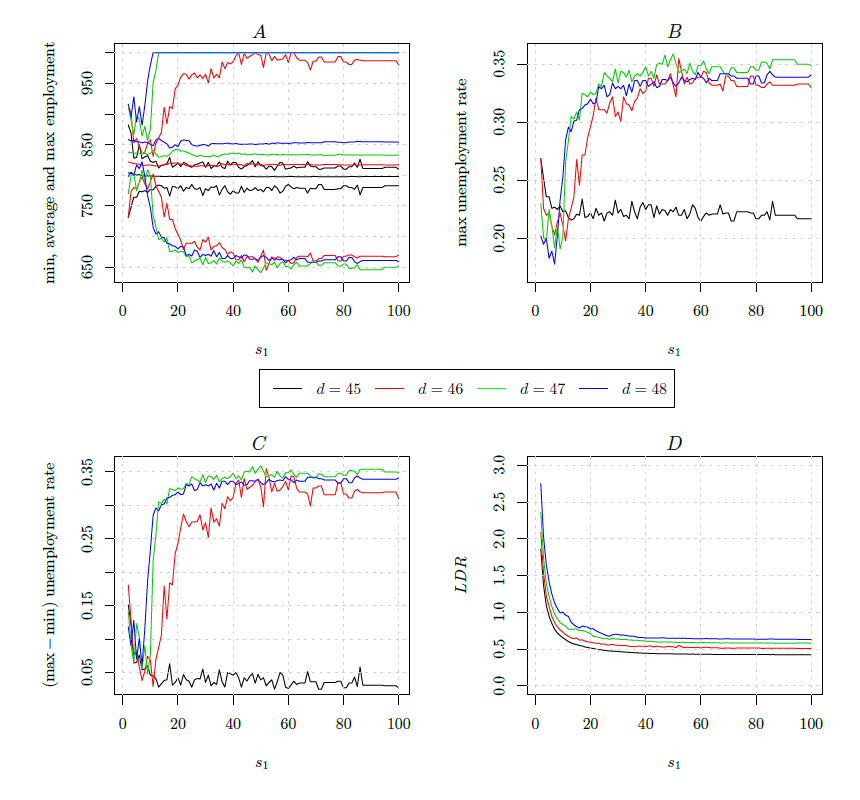
Overall, Figure 2 might be useful to a policy maker that faces the choice of the level of the unemployment dole. It suggests that a low level of the dole reduces employment fluctuations and implies a more stable banking sector.
We use the Loans-to-Deposits ratio (LDR) to report on the banking sector’s health. This ratio is taken as a liquidity indicator (Bonfin & Moshe 2014) and in some countries it is used as a prudential liquidity regulation measure (Sanya et al. 2012). Figure 2D shows how the LDR increases when the dole increase or s1 decreases; which in turn implies that these changes in the parameters both worsen the bank liquidity position.
In the following, we will provide a detailed description of the effect of changing the households’ willingness to borrow.
To this aim, we provide a detailed report for three specific levels of \(s_1\) : \(s_1\) = 6, \(s_1\) = 10 and \(s_1\) = 50. The first value minimizes employment’s fluctuations, but it represents a borderline case for bank liquidity. The second case (\(s_1\) = 10) can be thought of as an intermediate benchmark framework both for employment fluctuations and for bank liquidity. The third case (\(s_1\) = 50) corresponds to a safe bank liquidity position, but it is extreme for employment fluctuations. We recall that an increase in \(s_1\) weakens the borrowing attitude and promotes saving among households.
Table 3 presents the main results of the simulations run which adopt the three different values of \(s_1\); the other parameters are from the baseline parametrization reported in Tables 1 and 2. The reported values consider the averages over 2500 time periods: simulations last 3000 time step, but we discarded the first 500 periods in order to get rid of the transients and of the initialization dynamics of the simulation.
| Variables → | Unempl Rate | Consumption | Wealth | Loans | Deposits |
|---|---|---|---|---|---|
| Statistics ↓ | \(\langle{U_t}\rangle\) | \(\langle{C_{h,t}}\rangle\) | \(\langle{W_{h,t}}\rangle\) | \(\langle{L_{h,t}}\rangle\) | \(\langle{D_{h,t}}\rangle\) |
| \(s_1\)=6 | |||||
| mean | 18.23% | 60.88 | 55.66 | 2.26 | 57.61 |
| min | 13.2% | 57.62 | 47.08 | 0 | 0 |
| max | 22.8% | 63.17 | 62.5 | 3.26 | 82.59 |
| sd | 0.99% | 0.62 | 2.19 | 0.23 | 4.5 |
| IQR | 0.79 | 2.9 | |||
| \(s_1\)=10 | |||||
| mean | 18.35% | 60.88 | 72.28 | 1.04 | 72.9 |
| min | 14.2% | 57.59 | 59.67 | 0 | 0 |
| max | 22.6% | 63.77 | 81.63 | 2.14 | 112.7 |
| sd | 1.08% | 0.75 | 3.15 | 0.17 | 7.3 |
| IQR | 1.055 | 4.5 | |||
| \(s_1\)=50 | |||||
| mean | 18.3% | 60.9 | 99.3 | 2.26 | 57.6 |
| min | 0% | 48.49 | 0 | 0 | 0 |
| max | 35% | 74.53 | 160.2 | 3.2 | 82.6 |
| sd | 10.7% | 7.9 | 38.5 | 0.23 | 4.5 |
| IQR | 15.7 | 75.0 |
A first difference between the three cases is that the framework characterized by a lower willingness to borrow (\(s_1\) = 50) is more volatile compared to the other two, as confirmed by the inspection of the standard deviations for all the core variables under scrutiny.
Moreover, the third framework (\(s_1\) = 50) features a greater inequality in the distribution of wealth which is in turn mirrored by the distribution of consumption. Indeed, if we look at the Inter-Quantile Range measure (IQR), we see that it is higher for both consumption and wealth in presence of a lower willingness to borrow.
In order to deeply investigate the source and the role of inequality in the three frameworks, we report in Figure 3A the dynamics of the Gini index, \(G\) for the wealth distribution in a run for the three s1 values considered in this comparison.
Simulations with \(s_1\) = 6 exhibit more wealth inequality (on average) compared with the \(s_1\) = 10 and \(s_1\) = 50 scenarios; the average (rounded) values of the Gini index are respectively \(G_{s_1=6}=0.61\), \(G_{s_1=10}=0.48\) and \(G_{s_1=50}=0.29\). These values, in particular those observed in the cases of higher willingness to borrow, are in line with the Gini index observed in the empirical time series of several European countries. Summary statistics and the value of the Gini index for a set of European countries are reported in Table 5.
Considering the role played by credit in our framework, we take a closer look at the bank balance sheet in order to better understand the dynamics of the baseline scenarios. Figure 3 also reports the results of this investigation. We focus on the core financial variables and discuss the implications of their dynamics on the bank balance sheets’ health. We observe that in presence of high willingness to borrow the household sector (at the aggregate level) has a higher debt-to-income ratio (DTI-R) compared to the case in which households have a lower willingness to borrow. The DTI-R is in turn mirrored by a higher loans-to-deposits ratio (LDR) (see Figure 3B and C), which often presents values higher than 1; this means that the banking sector runs often in liquidity problems. These dynamics affect the bank’s balance sheet, as reported in Figures 3D, E and F. In the case of higher willingness to borrow, we observe that the bank often runs into liquidity problems due to the higher debt-to-income ratios and the LDR’s dynamics, while in the case of lower willingness to borrow (\(s_1\) = 10) the LDR ranges between 0.6 and 0.9, implying a healthier bank’s balance sheet.
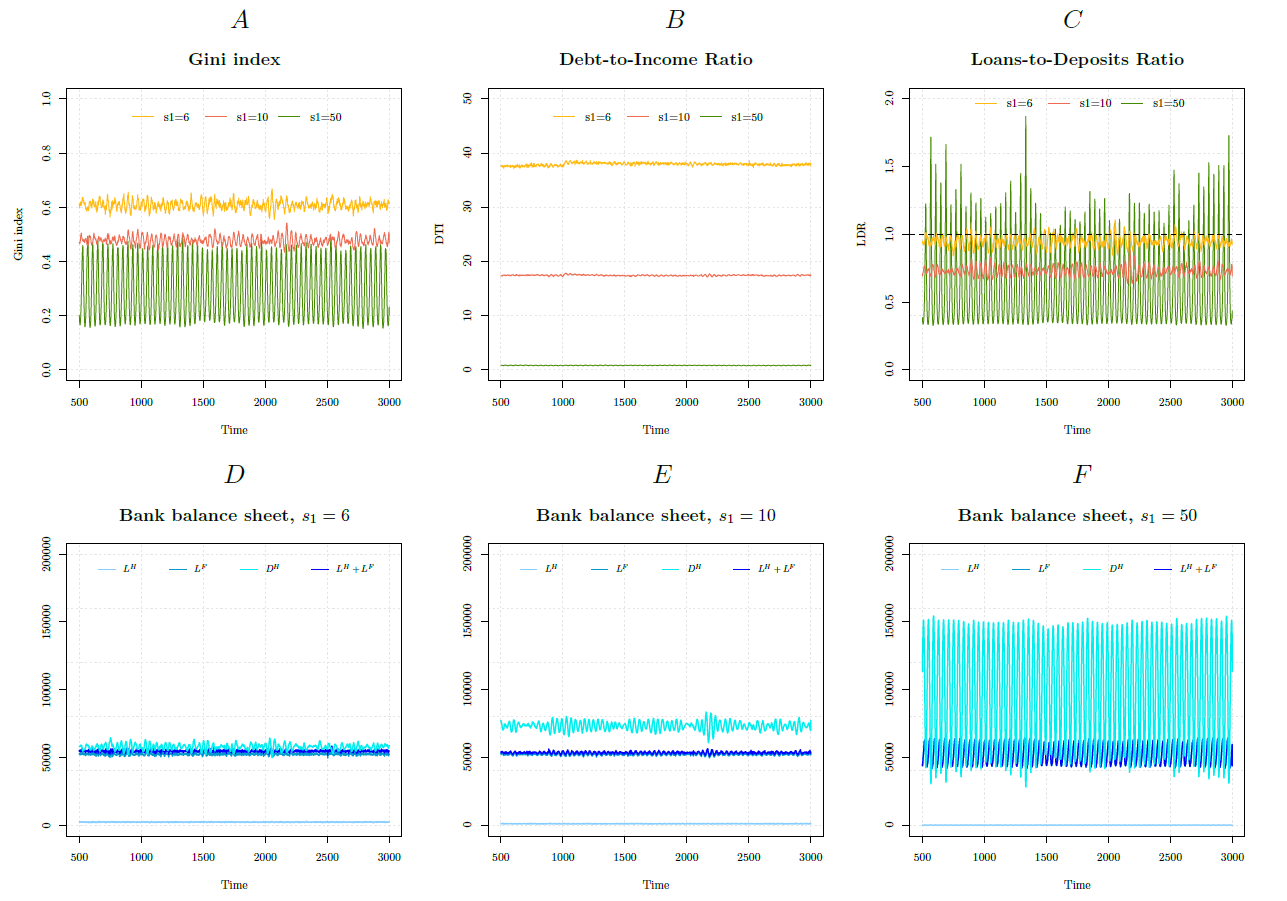
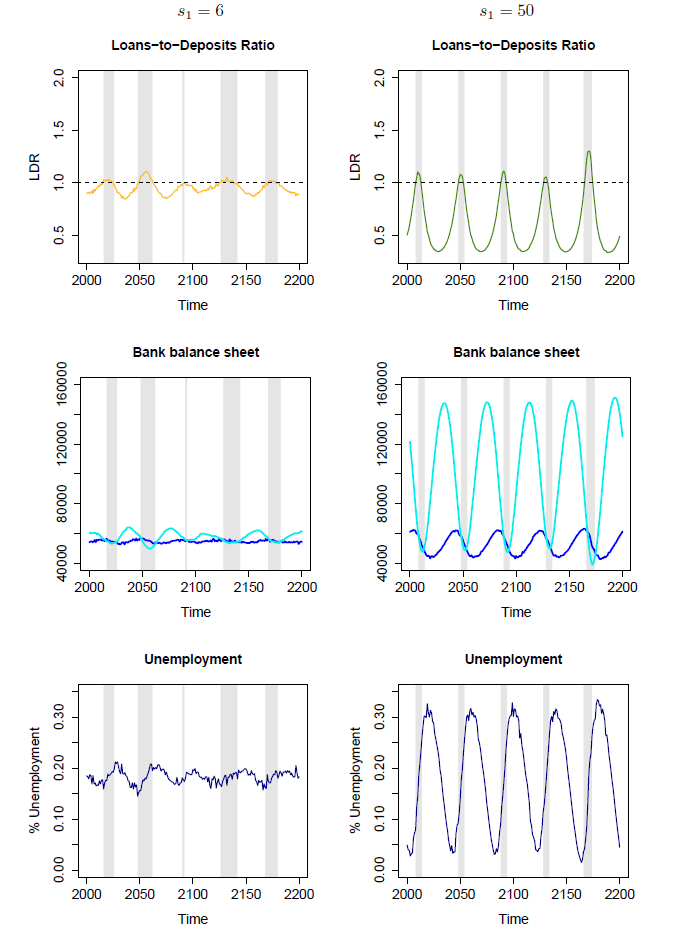
We deeper investigate the debt dynamics and their effects on the bank’s balance sheet by focusing on a subset of 200 time periods for the case of \(s_1\) = 6 and \(s_1\) = 50; we report them in Figure 4 where the gray stripes highlight the liquidity shortages’ time spans (LDR>1). During these periods, the deposits (light blue line) in the bank’s balance sheet are lower than aggregate loans (dark blue line), causing liquidity shortages. The credit cycles seem quite regular in the considered time span in both cases and the grey areas allow us to emphasize the duration of the fluctuations.
The focus over these dynamics in a subset of the overall simulation periods allows us to emphasize also another important feature of the model; namely that unemployment dynamics are strongly related to the credit cycle. Indeed, we observe that even in the presence of a higher willingness to borrow (\(s_1\) = 6), because of the precautionary saving motive at work in the household sector, consumers decide to decrease the demand for loans as the unemployment rate increases. In particular, Figure 4 clearly illustrates that unemployment dynamics drive the demand for loans: when the unemployment rate decreases, the demand for loans increase; in presence of a higher willingness to borrow across the population, this eventually leads to a higher LDR and to some peaks in the relationship between loans and deposits that result in liquidity shortages.
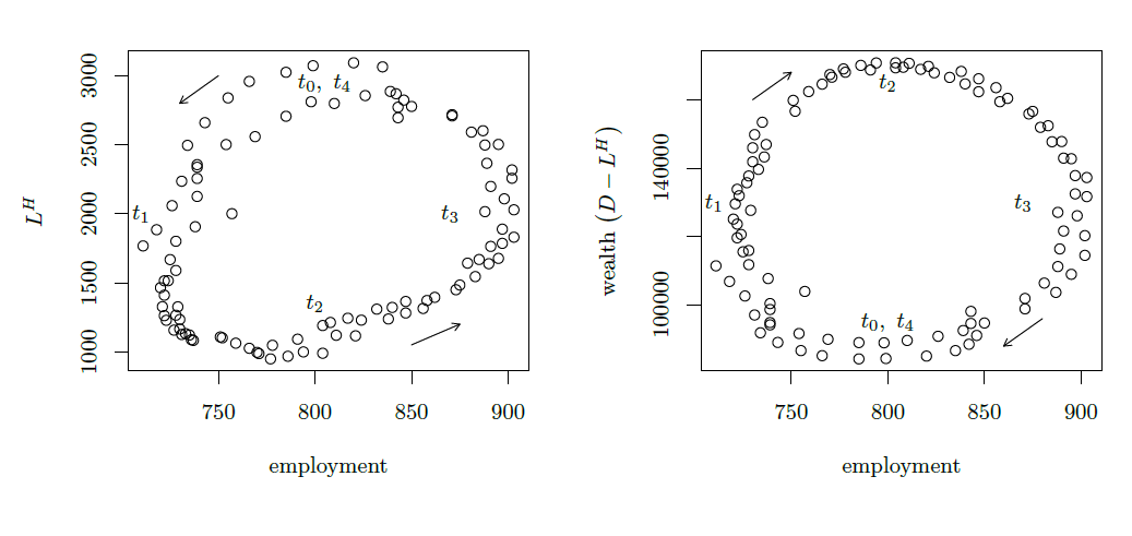
Focusing on the more volatile case \(s_1\) = 50, we provide in Figure 5 the phase diagrams that associate households’ financial variables (credit and wealth) to the employment level. To have a better under-standing of the ongoing dynamics, we add a time marker \(t\) to the figure. \(t_1\) denotes the trough of the business cycle. The arrows help to understand how the economy moves. During the recovery, it moves from \(t_1\) to \(t_2\) and then arrives at the top of the business cycle in \(t_3\). Following the time marker, we can see how during the recovery households continue the financial position improvement process started in the final part of the recession phase (since \(t_0\)). Indeed, starting from \(t_0\), which corresponds to the central periods of the recession, households’ debt start decreasing and wealth, also (and especially) thanks to deposits, increases. The process continues until the middle of the expansion (\(t_3\)) where the trends reverts signalling households’ will to move towards a more fragile financial position[11]. These movements of the agents financial position over the business cycle basically match those identified by Hyman Minsky as responsible for macroeconomic fluctuation (and more specifically, for financial crisis) in capitalistic economies (Minsky 1986).
Wealth distribution: comparing empirical and simulated distributions
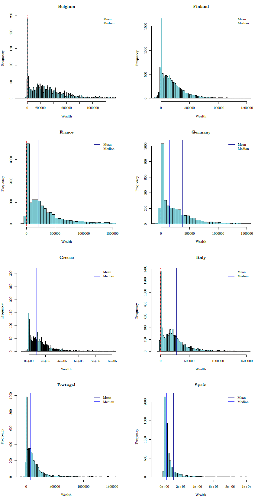
At this stage of our investigation and given the simple structure of our model, we report empirical and simulated wealth distributions for a visual comparison and leave a more quantitative investigation for future works. Empirical data are drown from the HFCS (European Household Finance and Consumption Survey) dataset[12]. It is a relatively new harmonized data set that collects household-level data on balance sheets, wealth and income distribution for 15 Euro Area countries from which we selected a set of countries: Germany, Spain, Italy, France, Belgium, Portugal, Finland and Greece.
For the comparison between artificial and empirical wealth distribution, we considered the derived variable net wealth \(DN3001\) which is computed as the sum of real and financial wealth net of total debt:
| $$DN3001=DA3001-DL1000.$$ |
| Data set | Description | Variable | Description |
| European data - HFCS | |||
| D1 | Derived variables | DN 3001 | Net wealth |
| DA 3001 | Total assets | ||
| DL 1000 | Total liabilities |
In Table 5, we report for each country the summary statistics of the net wealth distributions and the reference year of the survey for the set of considered EU countries. In order to have also a visual inspection of the whole net wealth distribution and perform a quick cross country comparison, we report in Figure 6 the plots with the densities, mean and median for each country mentioned above.
| Germany | Italy | Spain | Greece | Belgium | Portugal | France | Finland | |
| Reference year | 2010 | 2010 | 2008 | 2009 | 2009 | 2009 | 2009 | 2009 |
| Total numb. obs. | 3565 | 7951 | 6197 | 2971 | 2326 | 4404 | 15006 | 10989 |
| Minimum | -358500 | -44600 | -1143000 | -90950 | -420500 | -87500 | -404400 | -633600 |
| Maximum | 76300000 | 26130000 | 401100000 | 11700000 | 8408000 | 2708000 | 84410000 | 14720000 |
| Median | 148200 | 183500 | 287400 | 95700 | 272000 | 78450 | 207200 | 144300 |
| Mean | 377700 | 281300 | 1140000 | 147400 | 441200 | 173200 | 516300 | 230800 |
| 1stQ | 20000 | 41500 | 128700 | 18580 | 88780 | 16030 | 35400 | 24780 |
| 3rdQ | 388600 | 335000 | 721700 | 187600 | 510600 | 171800 | 469000 | 303800 |
| IQR | 368600 | 293500 | 593022 | 169066 | 421789 | 155729 | 433569 | 278993 |
| Gini coefficient | 0.72 | 0.59 | 0.78 | 0.6 | 0.6 | 0.70 | 0.71 | 0.62 |
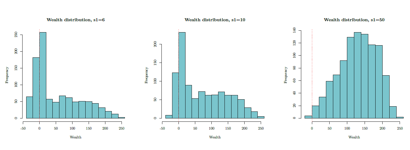
Wealth distributions obtained by simulations are reported in Figure 7. The reported distributions are taken at the latest time tick (\(t\) = 3000) of a simulation run for the three considered levels of s1. Because the wealth distribution evolves over time, much more information (in addition to the static pictures supplied by Figure 7) is needed to understand the dynamic of the wealth distribution. To this aim, in the Appendix, we provide the wealth_distribution_dynamics.mp4 video showing the dynamics under different parametrizations. The movements of the distribution are evident for high values of \(s_1\). The video shows that, for high \(s_1\), during economic upswings the mass on the medium and high values of the wealth distribution gradually moves to the left towards low and negative values. This is because deposits shrink and households ask for new credit. At the top of the business cycle, the wealth distribution is right skewed: it presents a high peak at low and negative values and is flat on its right side.
A comparison between the empirical distributions displayed in Figure 6 and those obtained from simulations (Figure 7) allows us to check whether the model presented in this paper can produce wealth distributions that are comparable to those observed in real economies. The visual inspection of Figure 7 shows similarities between the artificial distribution observed in the case of \(s_1\) = 6 and the wealth distribution of Germany, France and Finland. The distribution observed in the case of \(s_1\) = 10 shows instead similarities with the distribution observed for Greece, Italy and Belgium. The wealth distribution observed in the case of \(s_1\) = 50 instead does not show any similarity with real world data. The distributions shows indeed a left skew which is not present in real data. This finding is in line with the observation that the majority of European countries are characterized by a borrowing behavior in the household sector - which is in turn mirrored by higher debt to income ratios - that is better approximated by the scenarios with a higher willingness to borrow.
Considering that the main focus of the paper is on the left tail of the distribution, namely on negative wealth levels (debt) and their changes due to households’ willingness to borrow, we believe that being able to replicate it represents a promising result of the model at this stage of the research. However, more efforts are needed to provide a more sensible replication of the whole wealth distribution observed in real data, with particular regard to the right tail for which the bulk of the economic and econophysic literature (e.g. Chakraborti 2007; Yakovenko & Rosser 2009, for more details on this line of research), reports that it follows a power law[13]. We leave this investigation for future research.
Aggregate effects of different labor market matching mechanisms
In this section, we analyze the effects of different labor market matching mechanisms. As noted by Freeman (1998), adopting an agent-based approach to shape the labor market can help in studying the performance of the market. Indeed, it allows us to compare the outcomes of a model when the structure is imposed by the policymaker (centralized market) with that of a model in which the matching emerges from the bottom-up interactions between workers and firms (decentralized market)[14].
Our model can be used to perform such analysis by changing the \(SP\) and \(SR\) parameters. We consider three scenarios parametrized as reported in Table 6, whose implications can be easily understood by remembering equation (8). In the perfect information scenario, the production sector is able to identify the productivity of each worker; given the hiring mechanisms (the most productive workers are hired first), working positions are stable and they evolve slowly. In the realistic imperfections scenario, individual working positions can change in every period, and low productivity workers have the same possibility of getting a job than those characterized by high productivity. We define this scenario as “realistic” because of the ex-post observation that it allows for realistic macro and micro dynamics. The weak imperfections scenario makes that less productive workers are able to get a job, but with lower probabilities than those with high productivity.
| Matching mechanism | Signal productivity,SP | Signal random,SR |
|---|---|---|
| Perfect Information | 1 | 0 |
| Realistic Imperfections | 1 | 0.5 |
| Weak Imperfections | 1 | 0.05 |
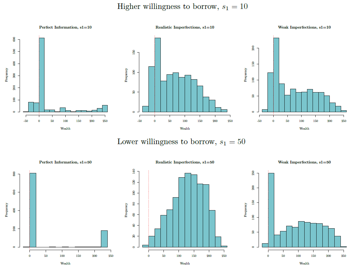
Figure 8 offers a visual representation of the labor market dynamics by considering the different matching mechanisms. We report time on the horizontal axis and workers’ productivity rank on the vertical axis: the lower the productivity, the higher the rank. As expected, in the scenario characterized by a matching mechanism based on perfect information the system is static and the employment (green) and unemployment (red) areas are compact and sharply delimited. As the graph emphasizes, unemployment is concentrated among less productive workers. In the realistic imperfections scenario, red and green pixels are uniformly mixed signaling a very dynamic labor market. Finally, the red gradually fades while the green intensifies moving from the top towards the bottom in the weak imperfections scenario.
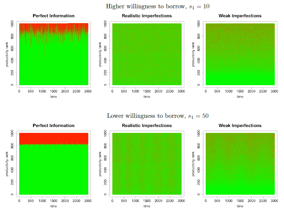
In Figure 9, we report the distribution of wealth corresponding to the matching mechanisms described in Figure 8. We observe that in the case of a matching mechanism based on perfect information the distribution is not positive skewed as observed in empirical distributions; rather it presents a peak on the lower side and another smaller peak on the right side. This particular shape of the distribution results from the hiring mechanism at work in this case according to which workers with lower productivity have less probabilities to be hired with respect to the workers characterized by higher productivity. Since productivity is considered in the determination of the wage level (see Equation 9) and affect thus the level of available income of each household, these dynamics have effects also on the distribution of wealth. Looking at the Gini Index in the case of \(s_1\) = 10 and \(s_1\) = 50 in presence of matching based on perfect information, we observe that it is on average equal to \(G_{s_1=10}=0.74\) and \(G_{s_1=50}=0.77\) which are consistently higher than those observed in the baseline scenario, i.e., \(G_{s_1=10}=0.48\)and \(G_{s_1=50}=0.29\) (see paragraph 3.17). This can be taken as an indirect proof that real world labor markets are characterized by imperfections. The visual inspection shows that the wealth distribution obtained from simulations gradually approaches the shape of the empirical one when imperfections grow in magnitude. The realistic imperfection case with a higher willingness to borrow is the most suitable setting to replicate the empirically observed wealth distribution.
Concluding remarks
The model presented in the paper has focused on behavioral features and financial choices that characterize the household sector and that can affect the shape of the business cycle. The model is composed of a production sector, a banking sector and a household sector populated by heterogeneous consumers that differ in many aspects: employment state, beliefs, wealth distribution, productivity and credit constraints. It is important to note that by considering this heterogeneity, we are able to analyze consumers’ behavior and their responses to changes to their wealth over changing macroeconomic conditions. Investigating these issues is relevant, especially during the recession phase of the business cycle, when policy makers face the challenge of designing stabilization policies.
The paper emphasized certain important issues related to the distribution of wealth and the implications of inequality, the concerns for which have been brought back by the Great Recession. Many authors have indeed observed that the emergence and unfolding of the financial crisis can be explained also by rising socio-economic inequality (see Iacoviello 2008; Fitoussi & Saraceno 2010; Galbraith 2012; VanTreeck 2013; Cynamon & Fazzari 2013, among others), with particular attention to the implications of the rising income inequality. In this paper, we rather focused on the implications of wealth inequality and reported extensive sensitivity analyses over the parameter that regulates the willingness to borrow \(s_1\).
By comparing three frameworks that differed in the \(s_1\) parameter, we found that, with a lively labor market, the one characterized by a lower willingness to borrow is more volatile compared to the other two characterized by a higher willingness to borrow. Moreover, it features a greater inequality in the distribution of wealth, which is in turn mirrored by the distribution of consumption. In order to gain a deeper understanding of the distributional issues at work in the model, we inspected also the dynamics of the Gini index over the whole simulation time periods. We found that the distribution of wealth is more concentrated in the framework characterized by high willingness to borrow, for which the observed average Gini index is \(G_{s_1=6}=0.61\), and less concentrated but more volatile in the case of lower willingness to borrow: \(G_{s_1=50}=0.29\).
This finding has some important implications for the stability of the banking sector and of the macro economy as a whole; indeed, it stresses that by pushing the LDR ratio too high and causing liquidity problems to the banking sector, the concentration of wealth can directly affect the stability of the system. Indeed, Figure 4 showed that the amplitude of the fluctuations are quite similar in the two scenarios, but the liquidity crises are longer in the presence of higher willingness to take on debt.
We also considered some possible (although very stylized) fiscal policy scenarios. In Section 3.4, Figure 8 suggested that a low level of the unemployment dole increases unemployment and, at the same time, it reduces employment fluctuations, also implying a more stable banking sector. This result can offer some insights to a policy maker who has to decide about the level of the unemployment dole over different phases of the business cycle.
After presenting and discussing sensitivity analysis over a set of parameters, the paper has reported the results of an ex-post validation exercise by comparing simulated and empirical wealth distributions. The paper stresses indeed the importance of matching stylized facts at the household level for thinking about the reaction of economies to recessions. In this, the availability of microeconomic data have been crucial for the macroeconomic insights they are able to provide. In this version of the model, microeconomic European data on the distribution of wealth retrieved from the HFCS dataset level have been considered. A visual inspection and comparison between empirical distributions and those obtained from simulations reveals shapes’ similarities in the case of the matching based on realistic imperfections. These results deserve however a more quantitative investigation that we leave for future works.
The effect of different levels of labor market imperfections on the wealth distribution is also analyzed.
In our model, the wealth distribution shape is different from the empirical one in the perfect information case, i.e. when the production sector can easily identify and hire most productive workers. Higher uncertainty on the employment state implied by labor market’s matching imperfections implies instead more hump shaped distributions. Using empirical data from the dataset discussed in Section 3.20, we observed that in these cases the shape of the French, Finnish, German and Italian wealth distributions can be generated by the model.
In conclusion, the model aims to provide a useful benchmark for grasping the main implications of the interaction between consumers’ wants (desired consumption), consumers’ beliefs (their expectations about their future income and employment state), the behavior of the banking sector (rationing) and the decision of the production sector (forecasting future demand). The structure of the model has been kept as simple as possible to clarify the mechanisms at work in the build up of consumer credit when we are in presence of precautionary saving motives. As a consequence, some important issues as bubbles linked to assets prices and monetary policies implications have been assumed away. Moreover, the model omits any role for a policy aimed at bringing the economy back to a healthy unemployment rate and does not consider, at this stage of the investigation, the possible macroeconomic implications of different banking regulations. We leave these investigations for future versions of the model aiming at incorporating a more sophisticated production sector and long run factors.
Acknowledgements
A previous version of this paper has been presented at the 11th edition of the Artificial Economics Conference, held in Porto on 3-4 September 2015. We would like to thank Tim Verwaart and Pedro Campos for editing this special section for JASSS.Notes
- For similar analysis on household debt using data from the Eurosystem Household Finance and Consumption Survey (HFCS) see Christelis et al. (2015). They consider two types of debt, namely col-lateralized debt (which include mortgages, home equity loans, and debts for other real estate) and non-collateralised debts (i.e. credit card debt, instalment loans, overdrafts and other loans). The main finding of the paper is an extensive cross-country heterogeneity in holdings of collateralised debt: whereas less than 20% of Austrian and Italian households hold collateralised debt, this number stands around 40% in Cyprus, the Netherlands and Luxembourg. Furthermore, in a comparison with US households, they find them to be consistently more indebted than European households. The prevalence of non-collateralized debt in US is substantially larger than in all other countries, with a particularly large gap for the case of non-collateralised debt, where more than 60% of U.S. households participate, in contrast to around 20%-50% for European households.
- Marginal propensity to consume is higher for households with lower levels of wealth (Carroll et al. 2014a).
- What is true for the whole must be true for all or some of its parts.
- The attributes of some parts of a thing are attributed to the thing as a whole.
- As discussed in LeBlanc et al. (2015), there is an important percentage of European households that report precautionary saving as an important reason for saving. Their investigation on a panel of European households collected in the HFCS dataset that elicits information on the role of several saving motives show that the percentage ranges between 89% in Netherlands and 42% in Germany.
- As discussed in Carroll et al. (2014a). In traditional precautionary saving models, because the employed consumer is always at risk of a transition into the unemployed state where income will be zero, the natural borrowing constraint that characterizes these models prevents the consumer from ever choosing to go into debt. An indebted unemployed consumer with zero income might indeed be forced to consume zero or a negative amount (incurring negative infinity utility) in order to satisfy the budget constraint.
- We take advantage of the facilities provided by The Apache Commons Mathematics Library 3.6 to code the
Extrapolator classof our model. For a more detailed description of the forecasting process, see theextraplator_compute.pdffile reporting the UML sequence graph of the Extrapolator class computation method. - In this paper we assume \(\psi_h\) Pareto distributed (\(\mathcal{P}(p_1,p_2)\)). We remember that the average of this distribution is given by (\((p_1p_2)/(p_1-1)\)). Parameters will be set in such a way that this average is constant.
- The model has been developed in Java taking advantage of the Repast functionalities. Full instructions for installing and running it are available at https://www.openabm.org/model/4990/.
- See Fagiolo et al. (2007) for a comprehensive discussion about empirical validation in DSGE and ABM models and Windrum et al. (2007) for a methodological appraisal of problems arising in validation.
- See the Appendix in which we provided the
employment_financial_phase_diagram.mp4video clip to visualise this dynamics. - Data and detailed information are available at https://www.ecb.europa.eu/pub/economic-research/research-networks/html/researcher_hfcn.en.html.
- However, as emphasized by Clauset et al. (2009) “the empirical detection and characterization of power laws is made difficult by the large fluctuations that occur in the tail of the distribution”.
- Usually, models of labor markets assume an exogenous (aggregate) matching function (Petrongolo & Pissarides 2001), often in the form of a Cobb-Douglass given that it can be easily log-linearized, thus estimated. Recently, the agent-based approach has been widely used in labor economics (Ballot & Taymaz 1997; Ballot 2002; Neugart & Richiardi 2012), especially in performing policy analyses (Dawid & Neugart 2011) which allows us to study the matching mechanism and the endogenous matching function (Neugart 2004; Phelps et al. 2002).
Appendix
Movie 1. The employment_financial_phase_diagram video
Movie 2. The wealth_distribution_dynamics video
References
ASSENZA, T., Delli Gatti, D. & Grazzini, J. (2015). Emergent dynamics of a macroeconomic agent based model with capital and credit. Journal of Economic Dynamics and Control, 50(January), 5–28. [doi:10.1016/j.jedc.2014.07.001]
BALLOT, G. (2002). Modeling the labor market as an evolving institution: model {ARTEMIS}. Journal of Economic Behavior & Organization, 49(1), 51 – 77.
BALLOT, G. & Taymaz, E. (1997). The dynamics of firms in a micro-to-macro model: The role of training, learning and innovation. Journal of Evolutionary Economics, 7(4), 435–457. [doi:10.1007/s001910050052]
BARBA, A. & Pivetti, M. (2009). Rising household debt: Its causes and macroeconomic implications—a long-period analysis. Cambridge Journal of Economics, 33(1), 113–137.
BONFIN, D. & Moshe, K. (2014). Liquidity risk in banking: Is there herding? Discussion Paper 2012-024, European Banking Center.
BROCK, W.A. & Hommes, C.H. (1997). A rational route to randomness. Econometrica, 65(5), 1059–1096.
BUYUKKARABACAK, B. & Valev, N. (2010). The role of household and business credit in banking crises. Journal of Banking & Finance, 34(6), 1247–1256 [doi:10.1016/j.jbankfin.2009.11.022]
CARDACI, A. & Saraceno, F. (2015). Inequality, financialisation and economic crisis: an agent-based model. Documents de Travail de l’OFCE 2015-27, Observatoire Francais des Conjonctures Economiques (OFCE): http://EconPapers.repec.org/RePEc:fce:doctra:1527.
CARROLL, C.D. (1992). The buffer-stock theory of saving: some macroeconomic evidence. Tech. Rep. 2, 61-156, Brookings Papers on Economic Activity. [doi:10.2307/2534582]
CARROLL, C.D. (2012). Representing consumption and saving without a representative consumer. In Measuring Economic Sustainability and Progress, NBER Chapters. National Bureau of Economic Research, Inc.
CARROLL, C., Sommer, M. & Slacalek, J. (2012). Dissecting saving dynamics: Measuring wealth, precautionary, and credit effects. IMF Working Papers 12/219, International Monetary Fund. [doi:10.5089/9781475505696.001]
CARROLL, C.D., Slacalek, J. & Tokuoka, K. (2014a). The distribution of wealth and the marginal propensity to consume. Tech. rep., ECB Working Paper No. 1655, Available at SSRN: http://ssrn.com/abstract=2404862.
CARROLL, C.D., Slacalek, J. & Tokuoka, K. (2014b). The distribution of wealth and the MPC: implications of new European data. Tech. rep., ECB Working Paper.
CHAKRABORTI, A. (2007). Econophysics: A brief introduction to modeling wealth distribution. Science and Culture, 73(3/4), 55.
CHALLE, E. & Ragot, X. (2016). Precautionary saving over the business cycle. The Economic Journal, 126(590), 135–164. [doi:10.1111/ecoj.12189]
CHRISTELIS, D., Ehrmann, M. & Georgarakos, D. (2015). Exploring differences in Household debt across Euro Area countries and the US. Tech. Rep. 2015-16, Bank of Canada Working Papers.
CLAUSET, A., Shalizi, C.R. & Newman, M. E.J. (2009). Power-law distributions in empirical data. SIAM Review, 51(4), 661–703. [doi:10.1137/070710111]
CLEVELAND, W., Grosse, E. & Shyu, W. (1992). ‘Local regression models.’ Chapter 8. In J.M. Chambers & T. Hasti (Eds.), Statistical Models. Wadsworth & Brooks/Cole.
CYNAMON, B.Z. & Fazzari, S.M. (2013). Inequality and household finance during the consumer age. Economics Working Paper Archive WP 752, The Levy Economics Institute. [doi:10.2139/ssrn.2205524]
DAWID, H. & Neugart, M. (2011). Agent-based models for economic policy design. Eastern Economic Journal, 37(1), 44–50.
EGGERTSSON, G.B. & Krugman, P. (2012). Debt, Deleveraging, and the Liquidity Trap: A Fisher-Minsky-Koo Approach. The Quarterly Journal of Economics, 127(3), 1469–1513. [doi:10.1093/qje/qjs023]
ERLINGSSON, E., Raberto, M., Stefansson, H. & Sturluson, J. (2013). ‘Integrating the housing market into an agent-based economic model.’ In A.Teglio, S.Alfarano, E.Camacho-Cuena & M.Ginés-Vilar (Eds.), Managing Market Complexity, vol. 662 of Lecture Notes in Economics and Mathematical Systems, (pp. 65–76). Springer Berlin Heidelberg.
FAGIOLO, G., Birchenhall, C. & Windrum, P. (2007). Empirical Validation in Agent-based Models: Introduction to the Special Issue. Computational Economics, 30(3), 189–194. [doi:10.1007/s10614-007-9109-z]
FITOUSSI, J. & Saraceno, F. (2010). Inequality and macroeconomic performance. Documents de Travail de l’OFCE 2010-13, OFCE.
FREEMAN, R.B. (1998). War of the models: Which labour market institutions for the 21st century? Labour Economics, 5(1), 1–24: http://ideas.repec.org/a/eee/labeco/v5y1998i1p1-24.html. [doi:10.1016/S0927-5371(98)00002-5]
GALBRAITH, J. K. (2012). Inequality and instability: A study of the world economy just before the great crisis. Oxford University Press.
GOURINCHAS, P. & Parker, J. (2001). The empirical importance of precautionary savings. Working paper series, NBER. [doi:10.1257/aer.91.2.406]
HAYASHI, F. & Prescott, E.C. (2002). The 1990s in japan: A lost decade. Review of Economic Dynamics, 5(1), 206–235.
HOMMES, C. (2006). ‘Heterogeneous agent models in economics and finance.’ In L. Tesfatsion & K.L. Judd (Eds.), Handbook of Computational Economics, vol.2 of Handbook of Computational Economics, chap.23, (pp. 1109–1186). Elsevier.
HOMMES, C. (2007). Bounded rationality and learning in complex markets. CeNDEF Working Papers 07-01, Universiteit van Amsterdam, Center for Nonlinear Dynamics in Economics and Finance.
HOMMES, C. (2011). The heterogeneous expectations hypothesis: Some evidence from the lab. Journal of Economic Dynamics and Control, 35(1), 1–24. [doi:10.1016/j.jedc.2010.10.003]
IACOVIELLO, M. (2008). Household debt and income inequality, 1963-2003. Journal of Money, Credit and Banking, 40(5), 929–965.
ITO, T. & Mishkin, F.S. (2006). ‘Two decades of Japanese monetary policy and the deflation problem.’ In Monetary Policy with Very Low Inflation in the Pacific Rim, NBER-EASE, Volume 15, (pp. 131–202). University of Chicago Press. [doi:10.7208/chicago/9780226379012.003.0005]
JORDÁ, O., Schularick, M. & Taylor, A.M. (2013). When credit crises bites back. Journal of Money, Credit and Banking, 45(2), 3–28.
KIRMAN, A. (2014). Is it rational to have rational expectations? Mind & Society, 13(1), 29–48. [doi:10.1007/s11299-014-0136-x]
KIRMAN, A.P. (1992). Whom or What Does The Representative Individual Represent. Journal of Economic Perspective, 6, 117–36.
KLÜGL, F. (2008). A validation methodology for agent-based simulations. In Proceedings of the 2008 ACM symposium on Applied computing, SAC ’08, (pp. 39–43). New York, NY, USA: ACM. [doi:10.1145/1363686.1363696]
KONIG, N. & Grossl, I. (2014). Catching up with the joneses and borrowing constraints: An agent-based analysis of household debt. Working paper, University of Hamburg, Department of socioeconomics.
KOO, R.C. (2013). Balance sheet recession as the ‘other half’ of macroeconomics. European Journal of Economics and Economic Policies, 10(2), 136–157: http://www.elgaronline.com/journals/ejeep/10-2/ejeep.2013.02.01.xml. [doi:10.4337/ejeep.2013.02.01]
LEBLANC, J., Porpiglia, A., Teppa, F., Zhu, J. & Ziegelmeyer, M. (2015). Household saving behaviour and credit constraints in the Euro area. Tech. rep., ECB Working Paper 1790.
MANDEL, A., Jaeger, C., Fuerst, S., Lass, W., Lincke, D., Meissner, F., Pablo-Marti, F. & Wolf, S. (2010). Agent-based dynamics in disaggregated growth models. Tech. Rep. 2010.77, CES working papers.
MINSKY, H.P. (1986). Stabilizing an Unstable Economy. New Haven and London: Yale University Press.
MUTH, J.F. (1961). Rational expectations and the theory of price movements. Econometrica, 29(3), 315–335. [doi:10.2307/1909635]
NEUGARTNeugart, M. (2004). Endogenous matching functions: an agent-based computational approach. Advances in Complex Systems, 07(02), 187–201.
NEUGART, M. & Richiardi, M. (2012). Agent based models of the labor market. WORKING PAPER SERIES 125, Laboratorio R.Revelli - Centre for Employment studies.
PERUGINI, C., Hölscher, J. & Collie, S. (2016). Inequality, credit and financial crises. Cambridge Journal of Economics, 40(1), 227–257.
PETRONGOLO, B. & Pissarides, C.A. (2001). Looking into the black box: A survey of the matching function. Journal of Economic Literature, 39(2), 390–431. [doi:10.1257/jel.39.2.390]
PHELPS, S., Parsons, S., Mcburney, P. & Sklar, E. (2002). ‘Co-evolution of auction mechanisms and trading strategies: Towards a novel approach to microeconomic design.’ In GECCO-02 Workshop on Evolutionary Computation in Multi-Agent Systems, (pp. 65–72).
RUSSO, A., Riccetti, L. & Gallegati, M. (2016). Increasing inequality, consumer credit and financial fragility in an agent based macroeconomic model. Journal of Evolutionary Economics, 26(1), 25–47. [doi:10.1007/s00191-015-0410-z]
SANYA, S., Mitchell, W. & Kantengwa, A. (2012). Prudential liquidity regulation in developing countries: A case study of Rwanda. Working Paper WP/12/20, IMF.
SEPPECHER, P. & Salle, I. (2015). Deleveraging crises and deep recessions: A behavioural approach. Applied Economics, 47(34-35), 3771–3790. [doi:10.1080/00036846.2015.1021456]
SIMON, H.A. (1955). A Behavioral Model of Rational Choice. The Quarterly Journal of Economics, 69(1), 99–118.
SKINNER, J. (1988). Risky income, life cycle consumption, and precautionary savings. Journal of Monetary Economics, 22(2), 237–255. [doi:10.1016/0304-3932(88)90021-9]
VANTREECK, H. (2013). Did inequality caused the US financial crisis? Journal of Economic Surveys, 28(3), 421–448.
WINDRUM, P., Fagiolo, G. & Moneta, A. (2007). Empirical validation of agent-based models: Alternatives and prospects. Journal of Artificial Societies and Social Simulation, 10(2), 8: https://www.jasss.org/10/2/8.html.
YAKOVENKO, V.M. & Rosser, J.B. (2009). Colloquium: Statistical mechanics of money, wealth, and income. Rev. Mod. Phys., 81, 1703–1725.
ZINMAN, J. (2014). Household Debt: Facts, Puzzles, Theories, and Policies. Nber working papers, National Bureau of Economic Research, Inc. [doi:10.3386/w20496]