
Introduction
Transport and mobility have recently become a prominent application areas for agent-based modelling (Chen & Cheng 2010). Models of transport systems offer an objective common ground for discussing policies and compromises (de Dios Ortúzar & Willumsen 2011), help understanding the underlying behaviour of these systems and aid in decision making and transport planning.
Large-scale, complex systems, set in various socio-demographic contexts and land-use configurations, are often modelled by simulating the behaviour and interactions of millions of autonomous, self-interested agents. Agent-based modelling paradigm generally provides a high level of detail and allows representing non-linear patterns and phenomena beyond traditional analytical approaches (Bonabeau 2002). Specific subclass of agent-based models, called activity-based models, addresses particularly the need for realistic representation of travel demand and transport-related behaviour. Unlike traditional analytical trip-based models, activity-based models view travel demand as a consequence of agent's needs to pursue various activities distributed in space. Consequently, understanding of travel decisions is secondary to the fundamental understanding of activity behaviour (Jones et al. 1990). Gradual methodological shift towards such a behaviourally-oriented modelling paradigm is evident and the activity-based models, such as TRANSIMS (Smith et al. 1995) or ALBATROSS (Arentze & Timmermans 2000), or their derivatives, are often employed within complex state-of-the-art transport models.
In order to produce dependable and useful results, any model needs to be valid. In fact, validity is often considered the most important property of models (Klügl 2009). The process of quantifying the validity by determining whether the model is an accurate representation of the studied system is called validation. Validation process needs to be done thoroughly and throughout all the phases of model development (Law 2009).
Despite the growing adoption of activity-based models and the generally acknowledged importance of model validation, validation processes for activity-based models in particular have not yet been standardized by a detailed methodological framework. Validation techniques and guidelines are addressed in most modelling textbooks (Law 2007; Balci 1994) and have even been instantiated in the form of a validation process for general agent-based models (Cooley & Solano 2011; Klügl 2009). However, such techniques are still too general to provide a concrete, practical methodology for the statistical validation of activity-based models. The only work concerned with statistical properties of activity schedules is a recent comparative framework designed for real-world travel diary collection systems (Prelipcean 2015).
In this paper, we address this gap and propose a validation framework called VALFRAM (Validation Framework for Activity-based Models), designed specifically to statistically quantify the validity of activity-based transport models. The framework relies on real-world transport behaviour data and quantifies the model validity in terms of clearly defined numeric validation metrics. More specifically, activity schedules generated by the modelled agents are matched to travel diary survey data sets and to the origin-destination matrices, and compared in terms of their temporal, spatial and structural properties. Resulting validity metrics values can be used not only to argue the usability of a given model and to compare it to the alternatives, but also to guide and accelerate the process of model development.
The rest of this article is organized as follows: In Section 2, we provide an overview of transport modelling, we introduce the activity-based modelling paradigm and place the VALFRAM framework into the context of existing validation methodology. In Section 3, we describe the framework and all its underlying validation tasks in detail. In Section 4, use the framework to quantify the validity of six different activity-based models and show that the framework itself behaves according to the expectations. Finally, in Section 5, we summarize our contributions.
Preliminaries
Transport Modelling Overview
Research in the area of transport modelling has always been in close relation with many branches of natural and technical, as well as social sciences (Csiszar & G 1999). Since 1970s, we have seen numerous attempts to study transport systems by mathematical methods and analytical modelling. An extensive overview of analytical modelling methodology, along with the corresponding mathematical background can be found in a monograph by (de Dios Ortúzar & Willumsen 2011). Early models of transport systems were largely based on mathematical programming and continuous approximations. The former technique relied on detailed data and numerical methods, whereas the latter relied on concise summaries of data and analytic models. (Geoffrion 1976) advocated the use of simplified analytic models to gain insights into numerical mathematical programming models. In a similar spirit, (Hall 1986) illustrates applications of discrete and continuous approximations, and notes that continuous approximations are useful to develop models that are easy for humans to interpret and comprehend. Overview and classification of continuous approximation models can be found in (Langevin et al. 1996).
However, analytical models were often too abstract for expressing relevant aspects in the structure and dynamics of transport systems. To deal with this shortcoming, the paradigm of simulation modelling has been adopted by the transport research community and has been employed in parallel with analytical approaches. In 1969, (Wilson et al. 1969) conducted a pioneer simulation-based study of the influence of the service area, demand density and number of vehicles on the behaviour of a transport system. Simulations have since then been extensively utilized in transport research as a powerful tool for the analysis of transport system's behaviour.
In these simulations, the system's behaviour could only be centralized and governed in a top-down manner by a single entity or mechanism. Any self-initiated interactions, communication or negotiation among individual actors was impossible, which severely limited their level of autonomy. To overcome these limitations, a new paradigm called Agent-based (simulation) modelling was introduced. Agent-based modelling has proven to be a highly valuable tool, especially when studying complex self-organizing systems in many domains (Klügl 2009). Transport systems modelled under this paradigm are implemented as multi-agent systems - i.e., composed of autonomous entities termed agents situated in a shared environment which they perceive and act upon, in order to achieve their own goals. Good examples of activity-based models of transport systems are AgentPolis (Čertický et al. 2015), SUMO (Behrisch et al. 2011) or TRANSIMS (Smith et al. 1995).
Activity-based Models
To deal with a specific but complex problem of transport demand modelling1, a new subclass of agent-based models emerged in 1980s, called activity-based models.
Activity-based models (Ben-Akiva et al. 1996) are multi-agent models (Macal & North 2010) in which the agents plan and execute so-called activity schedules - finite sequences of activity instances interconnected by trips. Each activity instance has assigned a specific type (e.g., work, school or shop), location, desired start time and duration. Trips between the activity instances are specified by their main2 transport mode (e.g., car or bike). The conceptual appeal of this approach originates from the realization that a desire to participate in activities is more basic than the travel that these participations entail (Bhat & Koppelman 1999). By placing primary emphasis on activites and focusing on sequences or patterns of activity behavior, such an approach can, for example, examine how people modify their activity behaviour (e.g. will they substitute more out-of-home activities for in-home activities in the evening if they arrived early from work due to a work-schedule change?).
An early work on the topic is represented by the CARLA model, developed as part of the first comprehensive assessment of behaviourally-oriented approach at Oxford (Jones et al. 1983), followed by STARCHILD, which was often referred to as the first operational activity-based model (McNally 1986). Later work is represented by the SCHEDULER model - a cognitive architecture producing activity schedules from long- and short-term calendars and perceptual rules (Gärling et al. 1994), TRANSIMS - an integrated system of travel forecasting models, including activity scheduler (Smith et al. 1995), ALBATROSS - the first model of complete activity scheduling process automatically estimated from data (Arentze & Timmermans 2000), or more recent SACSIM (Bradley et al. 2010).
Validation Methods
Validation methods in general are usually divided into two types:
- Face validation subsumes all methods that rely on natural human intelligence such as expert assessments of model visualizations. Face validation shows that model's behaviour and outcomes are reasonable and plausible within the frame of the theoretic basis and implicit knowledge of system experts or stakeholders. Face validation is in general incapable of producing quantitative, comparable numeric results. Its basis in implicit expert knowledge and human intelligence also makes it difficult to standardize face validation in a formal methodological framework. In this paper, we therefore focus on statistical validation.
- Statistical validation (sometimes called empirical) employs statistical measures and tests to compare key properties of the model with the data gathered from the modelled system (usually the original real-world system).
Other validation approaches might include role-playing validation (Ligtenberg et al. 2010), where the behavior of modelled agents is compared to that of human actors. In (Gore & Reynolds Jr 2008), Gore suggests a validation approach based on sensitivity analysis of model parameters in relation to emergent behaviours. Validation of models based on a range from theory-driven to evidence-driven approach is covered in (Moss 2008).
From a higher-level perspective, VALFRAM can be viewed as an activity-based model-focused implementation of the statistical validation step of a more comprehensive validation procedure for generic agent-based models, introduced in (Klügl 2009), as depicted in Figure 1. Besides the face and statistical validation, this procedure features other complementary steps such as calibration and sensitivity analysis.
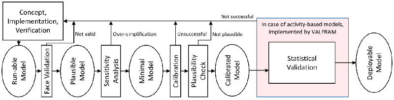
Being set in the context of activity-based modelling, the VALFRAM framework is concerned with the specific properties of activity schedules generated by agents within the model. These properties are compared to historical real-world data in order to compute a set of numeric similarity measures.
VALFRAM Description
In this section a detailed description of VALFRAM is given. We cover validation data, validation objectives and, finally, the statistics produced by VALFRAM.
Validation Data
A requirement for statistical validation of any model are the data capturing the relevant aspects of the reference system against which the model is validated. To validate an activity-based model, the VALFRAM framework requires two distinct data sets gathered in the modelled system:
- Travel Diaries: Travel diaries are usually obtained by long-term surveys (taking up to several weeks), during which participants log all their trips. The resulting data sets contain annonymised information about every participant (usually demographic attributes such as age, gender, etc.), and a collection of all their trips with the following properties: time and date, duration, transport mode(s) and purpose (the activity type at the destination). More detailed travel diaries also contain the locations of the origin and the destination of each trip. The location can be encoded either by coordinates (e.g., latitude and longitude) or by the identifier of a region. See Table 1 for an example of a travel diary for a single participant.
- Origin-Destination Matrix (O-D Matrix): The most basic O-D matrices (sometimes called trip tables) are simple two-dimensional square matrices containing the number of trips travelled between every combination of origin and destination locations during a specified time period (e.g., one day or one hour). The origin and destination locations are usually predefined, mutually exclusive zones covering the area of interest and their size determines the level of detail of the matrix. In real-world systems, O-D matrices may be obtained by roadside monitoring, household surveys or derived from mobile phone networks (Caceres et al. 2007).
| citizen id | household size | children in household | has car | has bike | |
|---|---|---|---|---|---|
| 0391 | 2 | 0 | false | false | |
| age | gender | student | education | driving license | pt card |
| 21 | male | true | secondary | true | true |
| activity | start | duration | location id | mode | |
| sleep | 0:00 | 9:45 | 551171 | node | |
| school | 10:05 | 5:40 | 550973 | pt | |
| lesure | 16:20 | 5:15 | 550103 | pt | |
| sleep | 22:15 | 1:45 | 551171 | walk |
VALFRAM Validation Objectives
The VALFRAM validation framework is concerned with a couple of specific properties of activity schedules produced by modelled agents. These particular properties need to correlate with the modelled system in order for the model to accurately reproduce the system's transport-related behaviour. At the same time, these properties can actually be validated based on available data sets - travel diaries and O-D matrices. In particular, we are interested in:
- A. Activities and their:
- 1.temporal properties (start times and durations),
- 2.spatial properties (distribution of activity locations in space),
- 3.structure of activity sequences (typical arrangement of successive activity types).
- B. Trips and their:
- 1.temporal properties (transport mode choice in different times of day; durations of trips),
- 2.spatial properties (distribution of trip's origin-destination pairs in space),
- 3.structure of transport mode choice (typical mode for each destination activity type).
VALFRAM Validation Statistics
To validate these properties of interest, we need to perform six validation steps (A1, A2, A3, B1, B2, B3), as depicted in Table 2 and detailed in the rest of this section. In each validation step, we compute specific numeric statistics. For all the statistics, the higher values indicate a larger difference between the model and validation set, i.e., lower accuracy.
A1. Activities in Time
In case of activities in time validation the problem is to compare the continuous univariate PDFs (Probability Density Functions) of start times and durations. Note that the method has to be nonparametric as we can make no assumptions about the distributions (which can be often, for example, multimodal). Well-established two-pair goodness-of-fit tests give us several possible statistics.
Kolmogorov-Smirnov two-sample statistic (Hollander et al. 2013) is defined as a maximum deviation between the empirical cumulative distribution functions (ECDFs) FM and FV which are based on the model and validation data distributions:
| $$d_{KS} = \sup_{x}|F_M(x)-F_V(x)|$$ | (1) |
| A. Activities | B. Trips | ||||
|---|---|---|---|---|---|
| Task | Dataset | Task | Dataset | ||
| 1. Time | Compare the distributions of start times and durations for each activity type using Kolmogorov-Smirnov (KS) statistic. | Travel diaries | a) Compare the distribution of selected modes by time of day and b) the distribution of travel times by mode using x2 and KS statistics. | Travel diaries | |
| 2. Space | Compare distribution of each activity type in 2D space using either kernelbased method or x2 statistic. | Space-aware Travel Diaries | Compute the distance between generated and realworld O-D matrix using RMSE. | Origin- Destination Matrix | |
| 3. Structure | a) Compare activity counts within activity schedules using x2 statistics. b) Compare distributions of activity schedule subsequences as n-grams profiles using x2 statistic. | Travel Diaries | Compare the distribution of selected transport mode for each type of target activity type using x2 statistics. | Travel Diaries |
Other possibilities are the statistics based on related Cramér-von Mises and Anderson-Darling two-sample tests (Hollander et al. 2013; Stephens 1986) defined using the sum of squared deviations of model and validation ECDFs.
For this step of VALFRAM, we recommend the Kolmogorov-Smirnov statistic as it is widely-used, easy to compute and intuitive. Nevertheless, we have done several experiments where all three statistics were compared and for most cases the results were qualitatively the same, e.g., dKSA < dKSB implied the same inequality for the other two statistics when applied to validation of any two models A and B using the same validation data. (see paragraph 4.13 for the details). For the convenience, we provide the implementation details of Kolmogorov-Smirnov statistic in the Appendix.
A2. Activities in Space
The comparison of activity distributions in space is performed separately for each activity type. In practice, there are two ways of defining of how the activities can be spatially defined. In the first case, each activity is assigned a continuous two-dimensional coordinate (e.g., latitude, longitude or other projection). The second possibility is based on regions, for example polygons3. While for the coordinate case we compare bivariate continuous PDFs, for the region-based one the validation is done by comparing the activity count per region. For the case of activities determined by the coordinates, we have developed a statistic based on the Root Mean Squared Error (RMSE) of sampled bivariate ECDFs in (Drchal et al. 2015). Unfortunately, the method has to be supplied a parameter which defines the sampling accuracy. We therefore recommend to use the z-score statistic developed by Duong (Duong et al. 2012) instead. The approach constructs a kernel-based density estimation of model and validation data and then computes their discrepancy similarly to Anderson-Darling test mentioned in the previous section.
If activities are tied to regions, we compare the activity counts per region. Well-established Pearson's x2 test statistic (Sokal & Rohlf 1994) can be employed. As in the previous case, the procedure is performed separately for each activity type. First, frequencies fMi and fVi for the region i are collected for both model and validation data. Validation data frequencies fVi are then used to get the count proportions pVi and, in turn, validation frequencies sVi are scaled to match the sum of model's frequencies \((\sum_i{s^V_i} = \sum_i{f^M_i})\). Using fMi and sVi, the x2 statistic is computed as:
| $$\chi^2 = \sum_i{(f^M_i - s^V_i)^2/s^V_i}$$ | (2) |
Note that, when applying to multiple models, one has to ensure that \(\sum_i{f^{M_j}_i}\) is the same for each model j for comparable values of \(\chi^{2}_{}\). For small validation datasets it may be inevitable to ignore regions with too few activity occurrences in order to limit the noise (see paragraph 4.17).
A3. Structure of Activities
In the previous steps, we examined the activity distributions in time and space. Here, we consider the composition of entire activity schedules. We propose a measure which compares distributions of activity counts (A3a) in activity schedules as well as a measure comparing the distribution of possible activity type sequences (A3b).
A3a. Activity Count
The comparison of activity counts in activity schedules is again based on the Pearson's \(\chi^{2}_{}\) test statistic. For both model and validation we collect frequencies fi. The value of fi is defined as the number of schedules in which the number of activity occurrences is exactly i for the selected activity type. We consider only frequencies for i > 0.
A3b. Activity Sequences
To compare activity sequence distributions we propose a method based on the well-established text mining techniques (Manning 1999; Cavnar et al. 1994). Particularly, we compare n-gram profiles using the \(\chi^{2}_{}\) statistic.
N-gram is a continuous subsequence of the original sequence having a length exactly n. Consider an example activity schedule consisting of the following activity sequence: \(\langle \texttt{none}, \texttt{sleep}, \texttt{school}, \texttt{leisure}, \texttt{sleep}, \texttt{none}\rangle\) 4. The set of all 2-grams (bigrams) is then: \(\{\langle \texttt{none}, \texttt{sleep}\rangle,\langle \texttt{sleep}, \texttt{school}\rangle, \langle \texttt{school}, \texttt{leisure}\rangle, \langle \texttt{leisure}, \texttt{sleep}\rangle, \langle \texttt{sleep}, \texttt{none}\rangle\}\).
We create an n-gram profile by counting the frequencies of all the n-grams in the range \(n\in\{1,2,\cdots,k\}\) for all the activity schedules, where k is the maximum number of activities found in validation activity schedules. All the N n-grams are then sorted by their counts in a decreasing order so that the counts are \(f_i \geq f_j\) for any two n-grams i and j where 1 ≤ i ≤ j ≤ N (for a tie fi = fj, one should sort in the lexicographical order to get deterministic results). We only work with a proportion P of n-grams having the highest count in the profile. More precisely, we take only the first M n-grams, where M is the highest value for which \(\sum_{i=1}^M{f_i} \leq P\sum_{i=1}^N{f_i}\) is true. This step is needed in order to remove the noise, similarly as described in paragraph 3.11.
In order to compare the n-gram profiles of model and validation data, we again employ \(\chi^{2}_{}\) statistic matching both profiles by the corresponding n-grams where only n-grams found in both profiles are considered. Note that the same number of schedules should be used when evaluating multiple models in order to get comparable \(\chi^{2}_{}\) values.
B1. Trips in Time
The validation of trips in time consists of two sub-steps: a comparison of mode distributions for a given time of day (B1a) and a comparison of travel time distributions for selected modes (B1b).
B1a. Modes by Time of Day
The comparison of mode distributions for a given time of day, for example \(p(\text{mode} | \text{time range})\), is again based on the \(\chi^{2}_{}\) statistic which is computed for mode frequencies of trips starting in a selected time interval. In (Drchal et al. 2015) we suggested to work with twenty four one-hour intervals per day which led to a large number of \(\chi^{2}_{}\) values per validation. For practical reasons we recommend a smaller number of longer intervals (as in paragraph 4.31). Note that the same number of trips should be used when evaluating multiple models in order to get comparable \(\chi^{2}_{}\) values.
B1b. Travel Times per Mode
Travel time distributions for modes \(p(\text{travel time}|\text{mode})\) are validated in the same way as activities in time (see validation step A1) using Kolmogorov-Smirnov statistic dKS.
B2. Trips in Space
In order to validate trip distributions in space, we propose a symmetrical dissimilarity measure based on O-D matrix comparison. The algorithm is realised in three consecutive steps. First, O-D matrices are rearranged to use a common set of origins and destinations. Second, both matrices are scaled to make trip counts comparable. Third, RMSE for all elements which have non zero trip count in either of the matrices is computed.
The algorithm starts with two O-D matrices: model matrix M and validation matrix V. Each element Mij (or Vij) represents a count of trips between origin i and destination j. The positional information (i.e., latitude/longitude, region identifier or other type of coordinates) is denoted \(m_i, m_j \in C_M\) for model and similarly \(v_i, v_j \in C_V\) for validation data where CM and CV are sets of all possible coordinates (e.g., all traffic network nodes, regions, etc.).
Note that in many practical cases \(C_M \neq C_V\). As an example we can have precise GPS coordinates generated by the model, however, only approximate or aggregated trip locations from validation travel diaries (i.e., regions). As we have to work with the same locations in order to compare the O-D matrices, we need to select a common set of coordinates C. In practice, this would be typically the validation data location set (C = CV) while all locations from CM must be projected to it by replacing each mi by its closest counterpart in C. This might eventually lead to resizing of the O-D matrix M as more origins/destinations might get aggregated into a single row/column.
In many cases, the total number of trips in M and V can be vastly different. The second step of the algorithm scales both M and V to a total element sum of one:
| $$M_{ij}' =\frac{M_{ij}}{\sum_{i}\sum_{j}M_{ij}}$$ | (3) |
| $$V_{ij}' =\frac{V_{ij}}{\sum_{i}\sum_{j}V_{ij}}$$ | (4) |
Finally, we compute the O-D matrix distance using the following equation:
| $$d_{OD} = \sqrt{\frac{\sum_{i}\sum_{j}\left(M'_{ij}-V'_{ij}\right)^2}{\left|\left\{(i,j):M'_{ij}>0 \lor V'_{ij}>0\right\}\right|}}$$ | (5) |
B3. Mode for Target Activity Type
The validation of the mode choice for a target activity type p(mode| activity type) is again based on the \(\chi^{2}_{}\) statistic. Here, we collect counts per each mode for each target activity of choice. The same number of activities should be used when evaluating multiple models in order to get comparable \(\chi^{2}_{}\) values.
VALFRAM Case Study
In general, we expect a statistical validation framework to meet the following three conditions:
- First, the framework needs to quantify the precision of validated models in a way which allows us to compare their accuracy in replicating different aspects of the behaviour of the modelled system.
- Second, the data required for the validation are available.
- Third, the validation metrics produced by the framework correlate with our expectations based on expert insight and face validation.
VALFRAM meets conditions 1 and 2 for activity-based models by explicitly expressing the spatial, temporal and structural properties of activities and trips, using only travel diaries and O-D matrices. To evaluate it with respect to condition 3, we have built six different activity-based models, formulated hypotheses about them based on our expert insight and used VALFRAM to validate them.
Evaluated Models
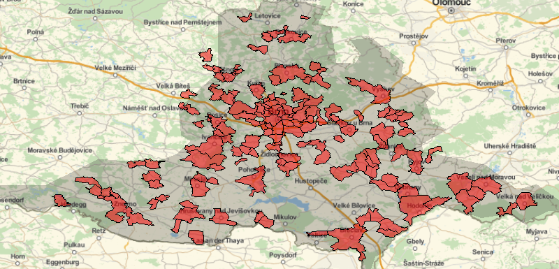
In this subsection, we describe the models used to evaluate VALFRAM. All the models considered in this case study target the South Moravian Region of Czech Republic populated by approximately 1.2 million citizens. An overview of the modelled area is depicted in Figure 2 where the red polygons denote regions for which validation data is available.
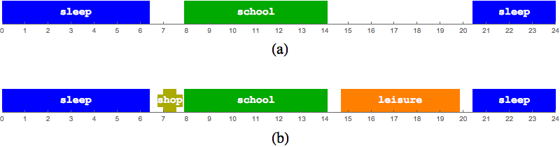
With a single exception (see below), all the models are inspired by the ALBATROSS model (Arentze & Timmermans 2000). We generate a single one-day activity schedule for all agents. However, for the sake of simplicity, we will focus mainly on a specific subset of the agents in this section - the student agents.5 The activity scheduling procedure of the ALBATROSS-inspired models is the following:
- The schedule skeleton is generated. A skeleton is a template for the final activity schedule consisting of fixed activities only. Fixed activities have locations (attractors) assigned beforehand, during population synthesis. In the schedules of the student agents, there are only two kinds of fixed activities: sleep and school. Start times and durations of these activities are generated by a probabilistic model. For an example of a skeleton, see Figure 3a.
- In order to produce the final activity schedule the skeleton's empty intervals are populated by flexible activities (leisure and shop activities). Specialised probabilistic models are used for determining both counts and durations for each flexible activity.
- All the flexible activities are assigned locations using attractor choice algorithm.
- The creation of the schedule is an iterative process in which the activities are repeatedly checked for being reachable by transport. To estimate trip durations as well as detailed composition of the trips we use a multimodal trip planner based on real transport network and time table data.
- The mode choice algorithm assigns a mode of transport to each trip between two subsequent activities. The currently supported modes are: pt (public transport), walk, car and bike.
- For an example of a final activity schedule see Figure 3b. Activity locations and selected modes are not shown.
As mentioned before, we use three types of probabilistic models as activity scheduler subcomponents. The first approximates PDFs of start times and durations for fixed activities, the second PDFs of flexible activity counts for each flexible activity type and the third one PDFs of flexible activity durations. In the past, we employed a simple Gaussian model in all cases The parameters of the Gaussian (mean and variance) were approximated by linear regression using the sociodemographic attributes of the agent. Currently we employ more advanced mixture of experts model of conditional probability as described in (Bishop 2006).
The attractor choice algorithm selects an appropriate location for each flexible activity in the schedule. Our current approach to attractor choice is to select a single attractor from a set of candidates lying in the vicinity of preceding and subsequent fixed activities. To demonstrate an influence of the attractor choice on spatial validity we also consider a simplified algorithm in which the set of candidates is limited to the vicinity of the main activity (school) only.
Our current approach to mode choice is based on a multinominal logistic regression (Bishop 2006). The logistic regression models the probability of selecting each mode based on agent's sociodemographic attributes, trip duration estimations and other inputs. Here we compare this approach to a simpler rule-based one which takes only trip duration estimations into account.
Apart from the ALBATROSS-based approaches, we evaluate VALFRAM on another kind of model, denoted LSTM. It represents a fully data-driven method based on Recurrent Neural Networks (RNNs). More specifically, the model employs fully-connected Long-Short Term Memory (LSTM) units (Hochreiter & Schmidhuber 1997) and several sets of softmax output units. Given the training dataset based on travel diaries, the model is trained to repetitively take current activity type and its end time as an input in order to produce a trip (including trip duration and mode) and the following activity (defined by its type and duration). LSTM model is currently unable to generate spatial component of the schedules (activity locations).
| designation | description | |
|---|---|---|
| MM | Baseline model using mixture of experts subcomponent probabilistic models for both fixed and flexible activities. | |
| LL | MM model predecessor using simpler linear probabilistic models for both fixed and flexible activities. | |
| ML | Using mixture of experts for fixed activities and a linear model for flexible activities. This model represents a development stage between LL and MM models. | |
| MMS | MM model with the simplified attractor choice method. Attractors are chosen in the vicinity of the main activity (school) only. MMS is expected to have inferior spatial properties when compared to MM. | |
| MMRMC | MM model with simplified rule-based mode choice method. | |
| LSTM | Fully data-driven model based on Long-Short Term Memory recurrent neural network architecture. Expected to give good results in generating activity sequences. Does not generate activity locations. |
Table 3 summarises the models used for this case study and their designations used in the following text. MM is a baseline model used in all the validation steps. LL and ML are its predecessors by means of probabilistic model subcomponents. MMS uses the simplified attractor choice algorithm and MMRMC uses the less advanced rule-based mode choice method. LSTM is an alternative approach to the above ALBATROSS-based models.
The same synthetic population was used for each model in the following subsections. The results are based on a random sample of 15,000 agents (each with one activity schedule) or on the randomly selected schedules containing 60,000 activities (same counts are needed when comparing multiple models using \(\chi^{2}_{}\) as mentioned above). We have found these numbers more than sufficient to eliminate an influence of the random selection. The amount of validation data was considerably lower: only 322 activity schedules and 865 trips of the students were available in the real-world travel surveys and O-D matrices. For the temporal and structural validation, this limited amount of validation data was satisfactory. For spatial validation, special measures were taken (see paragraph 4.23). Importantly, data used as training sets for the machine-learning subcomponents of the models were never used for validation purposes.
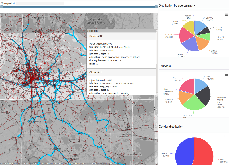
Figure 4 depicts an example output of the MM model. We use the visualization tool that allows us to analyse the activity schedules for selected agents as well as their sociodemographic distribution.
Results
In the following text we present selected results of the validation and comparison of the models. Note that all the VALFRAM steps (A1 through B3) are performed. A similar, less detailed, evaluation of VALFRAM was published in (Drchal et al. 2015). The results of the previous study cannot be compared to the results presented here due to new training and validation data sets.
Start Times and Durations
This section deals with validation of activity temporal properties: start times and durations.
Hypothesis: The performance of models will increase in order LL, ML and MM due to the use of more advanced mixture of experts subcomponent models.
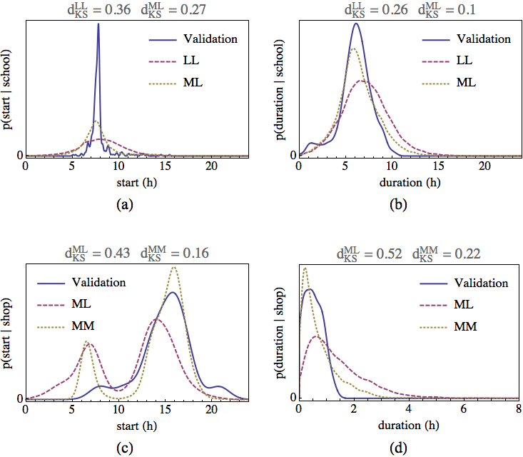
Table 4 shows a comparison of LL and ML in modelling start times and durations of fixed activities sleep and school (A1, activities in time). We have included all the discussed statistics (Kolmogorov-Smirnov, Cramér-von Mises and Anderson-Darling). We give related results for flexible activities leisure and shop for models ML and MM in Table 5. The tables clearly support the hypothesised improvements of ML over LL and MM over ML.
Moreover one can see that any statistic can be chosen in this case as \(d_{KS}^{ML} < d_{KS}^{LL}\), \(d_{CM}^{ML} < d_{CM}^{LL}\) and \(d_{AD}^{ML} < d_{AD}^{LL}\), where KS, CM and AD denote Kolmogorov-Smirnov, Cramér-von Mises and Anderson-Darling. Similar inequalities hold for validation of MM and ML models6. As we got qualitatively the same results for all kinds of models and also for comparisons of travel times per mode (B1b, see paragraph 4.28) we have decided to select Kolmogorov-Smirnov statistic for the reasons previously mentioned in paragraph 3.8. Figure 5 shows actual start time and duration PDFs for selected results.
| model | statistic | sleep | sleep | duration | duration |
|---|---|---|---|---|---|
| start time | duration | start time | duration | ||
| LL | Kolmogorov-Smirnov | 0.15 | 0.36 | 0.36 | 0.26 |
| ML | 4.9 x 10⁻² | 0.28 | 0.27 | 9.57 x 10⁻² | |
| LL | Cramér-von Mises | 1.7879 x 10³ | 43.5 | 12.3 | 7.9 |
| ML | 1.7876 x 10³ | 10.8 | 7.48 | 0.78 | |
| LL | Anderson-Darling | 13.7 | 117 | 60.6 | 38.6 |
| ML | 1.71 | 49.4 | 38.1 | 5.8 |
| model | statistic | leisure | leisure | shop | shop |
|---|---|---|---|---|---|
| start time | duration | start time | duration | ||
| ML | Kolmogorov-Smirnov | 0.66 | 0.26 | 0.43 | 0.52 |
| MM | 0.45 | 0.14 | 0.16 | 0.22 | |
| ML | Cramér-von Mises | 16 | 2.32 | 1.3 | 1.73 |
| MM | 6.71 | 0.31 | 7.8 x 10⁻² | 0.14 | |
| ML | Anderson-Darling | 102 | 11.7 | 7.34 | 10 |
| MM | 32.2 | 1.77 | 0.76 | 1.22 |
LSTM model produced varying but mostly inferior results when compared to the other models (data not presented). The analysis shown that this was most likely caused by inefficient encoding of continuous start time and duration PDFs with a combination of small training sets which led to overfitting.
Flexible Activity Counts and Sequences
Structural attributes of activity schedules are validated by means of activity count (A3a) and activity sequences (A3b) analysis.
Hypothesis: The performance of models will increase in order LL, ML, MM and LSTM due to use of more advanced mixture of experts subcomponent models in ALBATROSS-based models. LSTM model is expected to perform the best as it builds directly on data.
Table 6 shows activity count results for LL, ML, MM and LSTM. Note that only flexible activities (leisure and shop) are being considered here as the number of fixed activities is always constant in the current setup. The model performance increases in this order as hypothesised with an exception of MM and LSTM models for leisure activity. Further analysis has shown that these failures were caused by improperly trained models giving higher probabilities for two leisure activity instances. Both models can be most likely fixed by using a larger or more representative training set in future.
| model | leisure | shop |
|---|---|---|
| LL | 124 | 4.33 |
| ML | 87 | 3.73 |
| MM | 396 | 0.93 |
| LSTM | 108 | 0.27 |
Table 7 shows the result of activity sequence analysis (step A3b) for the same models using the proportion P = 0.9 and k = 11 (longest sequence in data). Although we have expected the same order of model precision as in the previous case, LSTM performed only second best. By a further analysis, we have found out that the reduced performance of the LSTM was caused by insufficient size of the training set.
Activity sequence analysis involves a comparison of activity n-gram frequencies. We have found the method very helpful for both model validation and calibration phases as by checking the n-grams having the highest frequency difference we were repeatedly able to quickly discover and fix the cause of model imprecision.
| LL | ML | MM | LSTM | \(\chi^{2}_{}\) | 10691 | 4406 | 1203 | 3983 |
|---|
Attractor Choice
This section evaluates VALFRAM's abilities of spatial validation (A2 and B2). We compare two approaches of attractor choice for flexible activities leisure and shop. Full attractor choice method employed by the MM model considers attractors in the vicinity of all fixed activities in the schedule while the simpler method (MMS model) takes only attractors close to the main activity location (school in the case of students) into account.
Hypothesis: MM model will be superior to MMS model.
There were only 105 activities available for as much as 47 regions in the validation dataset. In order to reduce the noise we have removed the regions which contained less than three activity records. Hence, the validation was done on 20 remaining regions.
Table 8 shows the result of MM and MMS models analysis of activities in space (A2). We give x2 for region determined activities where the model generated activity locations determined by latitude and longitude were transformed to the corresponding region identifiers. We also present the z-score of the kernel-based test method described in paragraph 3.9 using centroids of validation region polygons to generate continuous data. In all cases the results support the expected improvement of MM over MMS.
Related experiment considering trips in space distributions (B2) reveals similar results: \(d_{OD}^{MM} = 1.73\times 10^{-3} < d_{OD}^{MMS} = 1.78\times 10^{-3}\) which indicates that when compared with MMS, MM leads to OD-matrices better approximating validation data.
| model | leisure | leisure | shop | shop |
|---|---|---|---|---|
| \(\chi^{2}_{}\) | z-score | \(\chi^{2}_{}\) | z-score | |
| MM | 2574 | 2.65 | 213 | 6.42 |
| MMS | 3186 | 3.37 | 260 | 7.21 |
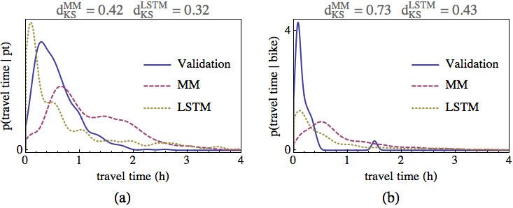
Travel Times per Mode
In this section we demonstrate VALFRAM's behaviour when comparing travel times per mode PDFs (B1b). All ALBATROSS-based models in this study depend on a same trip planner based on real transport network and time table data. Therefore we present only a comparison of the MM model to the LSTM one which infers the trip times solely from the data. Note that modelling the trip times directly from data avoids the imprecisions accumulated by a more complex model.
Hypothesis: LSTM model will be superior to MM model.
Table 9 supports this hypothesis: with an exception of walk mode, where the values of Kolmogorov-Smirnov statistic are the same, LSTM performs better than MM as expected. Figure 6 shows selected travel time PDFs so one can get an idea how the actual PDFs influence the value of the statistic.
| model | pt | walk | car | bike |
|---|---|---|---|---|
| MM | 0.42 | 0.37 | 0.44 | 0.73 |
| LSTM | 0.32 | 0.37 | 0.31 | 0.43 |
Mode Choice
This section compares the original rule-based mode choice method (MMRMC model) to the current mode choice method based on machine learning techniques (MM model). We add also the results for LSTM for completeness.
Hypothesis: The performance of models will increase in order MMRMC, MM. LSTM model has no access to trip-planning data (i.e., transport network, timetables) which considerably influences the mode choice. This should make its performance lower compared to the other two models provided the mode choice methods and the trip planner used by MM and MMRMC are accurate enough. While ALBATROSS-based models optimize the whole daily activity schedules, LSTM model works sequentially and schedules new activity based only on the previous ones. Therefore, it will be less precise towards the end of the day.
Figure 7 summarises the distribution of modes by time of a day (B1a) showing the expected superiority of MM over MMRMC. We present mode distributions as well as \(\chi^{2}_{}\) values for five four-hour intervals although other partitionings are possible. The interval 0:00-4:00 is not shown as there were not enough validation data for all modes to compute \(\chi^{2}_{}\)statistics. The rule-based method chooses an available mode having a shortest trip duration which is clearly demonstrated by students using bicycles excessively in Figure 7b.
With an exception of 16:00-20:00 interval LSTM gives the best results of all. Analysis shown that while the trip planner used by MM and MMRMC models is reasonably accurate the mode choice methods are not (e.g., notice how MM model overestimates the walk over the pt mode).
Note, however, that LSTM model precision decreases towards the end of the day, as expected, which can be explained by accumulating errors when sequentially constructing the activity schedules. This phenomenon can be better demonstrated for shorter validation intervals (e.g., one hour).
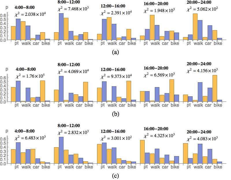
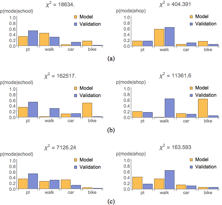
In Figure 8 we compare mode choice for target activity type (B3) using the same models MM, MMRMC and LSTM. Again, the lower values of \(\chi^{2}_{})\ indicate the improvement of MM over MMRMC. LSTM shows its superiority over both other models.
Discussion of Results
The results given in the previous sections shown the hypothesised increase of performance for models gradually more dependent on mixture of experts subcomponent models (in order LL, ML and MM). Comparison of MM model with MMS and MMRMC using simplified approaches to attractor and mode choice demonstrated that the improved methods are indeed beneficial. Although currently unable to generate activity locations, LSTM model was shown to be a promising approach. However, more efficient encoding of continuous PDFs for start times and durations should be considered in the future.
Spatial validation (mostly the step A2) suffered from the insufficient size of the validation dataset where the number of validated regions has to be substantially reduced. Although this currently limits us from the proper assessment of our models, it is not an issue from the VALFRAM methodology evaluation perspective.
Most VALFRAM steps return multiple statistic values (e.g., B1a, modes by time of day gives a \(\chi^{2}_{i}\) value for each defined interval i) which can be impractical. A possible solution is to marginalise the validated PDFs, i.e., evaluate \(p(\text{mode})\) instead of \(p(\text{mode} | \text{time range})\). For \(\chi^{2}_{}\) statistics there is another possibility of computing a single statistic value as \(\chi^2 = \sum_i{\chi_i^2}\) is the value of the statistic for component i. Such aggregations would, however, discard important information.
Conclusion
We have introduced a detailed methodological framework for data-driven statistical validation of multiagent activity-based models. The VALFRAM framework compares activity-based models against real-world travel diaries and origin-destination matrices. The framework produces several validation statistics quantifying the temporal, spatial and structural validity of activity schedules generated by the model. These values can be used to assess the accuracy of the model, guide its development, or compare it to other models. We have utilized the VALFRAM framework to validate and compare six different activity-based models of the same real-world region, populated by approximately 1 million inhabitants. The framework identified strong and weak aspects of each model with accordance to the insight of human experts, thus confirming its viability and usefulness. VALFRAM presents the first methodological statistical validation framework designed specifically for activity-based models (even though some parts of VALFRAM, like spatial validation of activities or activity sequence validation, could also prove usable for more general agent-based models).
Acknowledgements
This work was funded by Ministry of Education, Youth and Sports of Czech Republic (grants no. 7E12065 and LD12044), Technology Agency of the Czech Republic (grant no. TE01020155) and by the European Union Seventh Framework Programme FP7/2007-2013 (grant agreement no. 289067). Access to computing and storage facilities owned by parties and projects contributing to the National Grid Infrastructure MetaCentrum, provided under the programme "Projects of Large Research, Development, and Innovations Infrastructures" (CESNET LM2015042), is greatly appreciated. This work was also supported by The Ministry of Education, Youth and Sports from the Large Infrastructures for Research, Experimental Development and Innovations project "IT4Innovations National Supercomputing Center - LM2015070".Notes
- Activity-based models were an alternative to traditional four-step travel demand models created in 1950s.
- In general, the trips between activities can be multi-modal. In such case,we denote themodeof the longest leg (in terms of travel distance or time) as the “main mode” and denote the whole trip by it.
- This possibility was not covered in the first version of VALFRAM (Drchal et al. 2015).
- Note that "none" activities are added to the beginning and the end of the activity schedule in order to preserve the information about the initial/terminal activity.
- We call the agents with at least one school activity and no work activities the students. There are unnecessarily many non-student agents with overly complex schedules. While we do not have a representative validation set for the whole population we have it for the students. For the purposes of this case study, it is sufficient to focus on a subset of all the agents.
- This observation does not apply generally. While experimenting with other models (results not here) we have came across several cases when the order of the values was different for pairs of statistics. Nevertheless this happened for very similar models only.
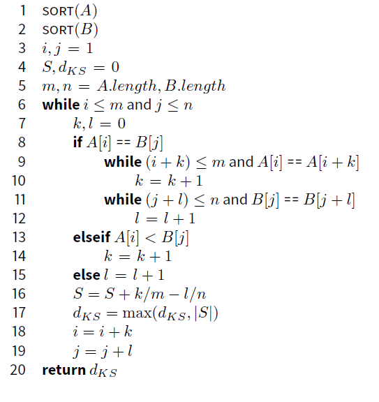
Appendix: Kolmogorov-Smirnov Statistic
The Kolmogorov-Smirnov deviation statistic is implemented in many software packages (e.g., R, Wolfram Mathematica, MATLAB). We give the pseudocode for convenience. The function Kolmogorov-Smirnov-Max-Deviation expects two arrays A and B of values as its input (activity start times, durations or trip durations in our case). The implementation is loosely based on (Monahan 2011).
References
ARENTZE, TIMMERMANS, H. (2000). Albatross: a learning based transportation oriented simulation system. Eirass Eindhoven.
BALCI, O. (1994).Validation, verification, and testing techniques throughout the life cycle of a simulation study. Annals of operations research, 53 (1), 121-173.
BEHRISCH, M., BIEKER, L., ERDMANN, J. & KRAJZEWICZ, D. (2011). Sumo - simulation of urban mobility. In: The Third International Conference on Advances in System Simulation (SIMUL 2011), Barcelona, Spain.
BEN-AKIVA, M., BOWMAN, J. L. & GOPINATH, D. (1996). Travel demand model system for the information era. Transportation 23 (3), 241-266.
BHAT, C. R. & KOPPELMAN, F. S. (1999). Activity-based modeling of travel demand. In: Handbook of transportation Science. Springer, pp. 35-61.
BISHOP, C. M.(2006).Pattern Recognition and Machine Learning (Information Science and Statistics). Secaucus, NJ, USA: Springer-Verlag New York, Inc.
BONABEAU, E. (2002). Agent-based modeling: Methods and techniques for simulating human systems. Proceedings of the National Academy of Sciences 99 (suppl 3), 7280-7287.
BRADLEY, M., BOWMAN, J. L. & GRIESENBECK, B. (2010). SACSIM: An applied activity-based model system with fine-level spatial and temporal resolution. Journal of Choice Modelling, 3 (1), 5-31.
CACERES, N., WIDEBERG, J. & BENITEZ, F. (2007). Deriving origin destination data from a mobile phone network. IET, 1 (1), 15-26.
CAVNAR, W. B., TRENKLE, J. M. et al. (1994). N-gram-based text categorization. Ann Arbor MI, 48113 (2), 161-175.
ČERTICKý, M., DRCHAL, J., CUCHý, M. & JAKOB, M. (2015). Fully agent-based simulation model of multimodal mobility in european cities. Proceedings of the 4th International Conference on Models and Technologies for Intelligent Transportation Systems (MT-ITS 2015).
CHEN, B. & CHENG, H. H. (2010). A review of the applications of agent technology in traffic and transportation systems. IEEE Transactions on Intelligent Transportation Systems, 11 (2), 485-497.
COOLEY, P. & SOLANO, E. (2011). Agent-based model (ABM) validation considerations. In: Proceedings of the Third International Conference on Advances in System Simulation (SIMUL 2011). Citeseer.
CSISZAR, C. G, W. (1999). Modeling of computer integrated transportation. Periodica Polytechnica Transportation Engineering, 27 (1-2), 43-59.
DE DIOS ORTúZAR, J. & WILLUMSEN, L. (2011). Modelling Transport. Wiley: http://books.google.cz/books?id=r7P0b8IdQRwC.
DRCHAL, J., ČERTICKý, M. & JAKOB, M. (2015). Data driven validation framework for multi-agent activity-based models. CoRR, abs/1502.07601: http://arxiv.org/abs/1502.07601.
DUONG, T., GOUD, B. & SCHAUER, K. (2012). Closed-form density-based framework for automatic detection of cellular morphology changes. PNAS, 109 (22), 8382-8387,
GäRLING, T., KWAN, M.- P. & GOLLEDGE, R. G. (1994). Computational-process modelling of household activity scheduling. Transportation Research Part B: Methodological, 28 (5), 355-364.
GEOFFRION, A. M. (1976). The purpose of mathematical programming is insight, not numbers. Interfaces, 7 (1), 81-92.
GORE, R. REYNOLDS, Jr, P.F. (2008). Applying causal inference to understand emergent behavior. In: Proceedings of the 40th Conference on Winter Simulation.
HALL, R. W. (1986). Discrete models/continuous models. Omega, 14 (3), 213-220.
HOCHREITER, S. & SCHMIDHUBER, J. (1997). Long short-term memory. Neural computation, 9 (8), 1735-1780.
HOLLANDER, M., WOLFE, D. A. & CHICKEN, E. (2013). Nonparametric Statistical Methods. Wiley, 3rd ed.
JONES, P. M., DIX, M. C., CLARKE, M. I. & HEGGIE, I. G. (1983). Understanding travel behaviour. Monograph.
JONES, P. M., KOPPELMAN, F. & ORFEUIL, J.-P. (1990). Activity analysis: State-of-the-art and future directions. Developments in dynamic and activity-based approaches to travel analysis , 34-55.
KLüGL, F. (2009). Agent-based simulation engineering. Ph.D. thesis, Habilitation Thesis, University of Würzburg.
LANGEVIN, A., MBARAGA, P. & CAMPBELL, J. F. (1996). Continuous approximation models in freight distribution: An overview. Transportation Research Part B: Methodological, 30 (3), 163-188.
LAW, A. M. (2007). Simulation modeling and analysis, 4th edition. McGraw-Hill New York.
LAW, A. M. (2009). How to build valid and credible simulation models. In: Simulation Conference (WSC), Proceedings of the 2009 Winter. IEEE.
LIGTENBERG, A.,VAN LAMMEREN, R. J., BREGT, A. K. & BEULENS, A. J. (2010). Validation of an agent-based model for spatial planning: A role-playing approach. Computers, Environment and Urban Systems, 34 (5), 424-434.
MACAL, C. M. & NORTH, M. J. (2010). Tutorial on agent-based modelling and simulation. Journal of simulation, 4(3), 151-162.
MANNING,C. D. (1999). Foundations of Statistical Natural Language Processing. MIT press.
McNALLY, M. G. (1986). On the formation of household travel/activity patterns: a simulation approach. Tech. rep.
MONAHAN, J. F. (2011). Numerical Methods of Statistics. Cambridge University Press, 2nd ed.
MOSS, S. (2008). Alternative approaches to the empirical validation of agent-based models. Journal of Artificial Societies and Social Simulation 11 (1), 5: https://www.jasss.org/11/1/5.html.
PRELIPCEAN, A. C. (2015). Comparative framework for activity-travel diary collection systems. Proceedings of the 4th IEEE International Conference on Models and Technologies for Intelligent Transport Systems (MT-ITS 2015).
SMITH, L., BECKMAN, R., ANSON, D., NAGEL, K. & WILLIAMS, M. E. (1995). TRANSIMS: Transportation analysis and simulation system. In: 5th National Conference on Transportation Planning Methods Applications-Volume II.
SOKAL, R. R. & ROHLF, F. J. (1994). Biometry: The Principles and Practices of Statistics in Biological Research. W. H. Freeman, 3rd ed.
STEPHENS, M. A. (1986). Tests based on EDF statistics. Goodness-of-fit Techniques, 68, 97-193.
WILSON, N. H. M., SUSSMAN, J., GOODMAN, L. & HIGNNET, B. (1969). Simulation of a computer aided routing system (cars). In: Proceedings of the third conference on applications of simulation. Winter Simulation Conference.