
 Abstract
- A large number of complex hypotheses exists that aim to explain aspects of the Roman economy, consisting of many explanatory factors that are argued to affect each other. Such complex hypotheses cannot be compared or tested through the traditional practice of qualitative argumentation and comparison with selected small sets of written and material sources alone. Moreover, these hypotheses often draw on different conceptual frameworks to abstract the same past phenomenon under study, hampering formal comparison. There is a need in the study of the Roman economy for more formal computational modelling for representing and comparing the many existing conceptual models, and for testing their ability to explain patterns observed in archaeological data where possible. This paper aims to address this need. It argues that communicating the potential contribution of computational modelling to scholars of the Roman economy should focus on providing theoretically well-founded arguments for the selection of the included and excluded variables, the conceptualisation used, and to address those elements of conceptual models that are at the forefront of scholarly debates. This approach is illustrated in this paper through MERCURY (Market Economy and Roman Ceramics Redistribution, after the Roman patron god of commerce), an agent-based model (ABM) of ceramic tableware trade in the Roman East. MERCURY presents a representation of two conflicting conceptual models of the degree of market integration in the Roman Empire, both of which serve as potential explanations for the empirically observed strong differences in the distribution patterns of tablewares. This paper illustrates how concepts derived from network science can be used to abstract both conceptual models, to implement these in an ABM and to formally compare them. The results of experiments with MERCURY suggest that limited degrees of market integration are unlikely to result in wide tableware distributions and strong differences between the tableware distributions. We conclude that in order for the discussion on the functioning of the Roman economy to progress, authors of conceptual models should (a) clearly define the concepts used and discuss exactly how these differ from the concepts used by others, (b) make explicit how these concepts can be represented as data, (c) describe the expected behaviour of the system using the defined concepts, (d) describe the expected data patterns resulting from this behaviour, and (d) define how (if at all) archaeological and historical sources can be used as reflections or proxies of these expected data patterns.
- Keywords:
- Roman Economy, Network Science, Economics, Archaeology, Ceramics, History
Introduction
- 1.1
- The vast amounts of Roman pottery found on sites throughout the former Roman Empire are the archaeologist's main source of data used to investigate the functioning and performance of the Roman economy. However, so far the study of the Roman economy through pottery distributions has been dominated by exploratory data analysis and conceptual models (hypotheses). The undoubted complexity of the real past phenomenon that is the Roman economy and the many factors that played a role in its functioning and performance have led scholars of the Roman economy to focus on qualitative evaluation of models and comparison with selected small sets of written and material sources alone. There is an almost complete absence of applications or approaches that allow for different conceptual models to be formally compared or tested. There is a need in the study of the Roman economy for more formal computational modelling for representing and comparing the many existing conceptual models, and for testing their ability to explain patterns observed in archaeological data where possible. Moreover, the ability of this approach to evaluate many explanatory factors through experimentation and how it can contribute to ongoing qualitative debates need to be illustrated.
- 1.2
- This paper aims to address this need by presenting a computational modelling approach to the Roman economy and focusing on providing theoretically well-founded arguments for the selection of the included and excluded variables, the conceptualisation used, and to address those elements of conceptual models that are at the forefront of scholarly debates. We believe this approach and argumentation will facilitate communication of the potential of this approach to scholars of the Roman economy and enable it to make constructive contributions to ongoing debates.
- 1.3
- This approach is illustrated in this paper through MERCURY (Market Economy and Roman Ceramics Redistribution, after the Roman patron god of commerce), an agent-based model (ABM) of ceramic tableware trade in the Roman East, developed to illustrate the potential of computational modelling for the study of the Roman economy. It aims to abstract aspects of two conflicting conceptual models of the functioning of the Roman trade system using comparable network science concepts. This paper places a strong emphasis on the conceptualisation and implementation of MERCURY, and additionally describes the sensitivity analysis measuring effects of changing independent variables on the resulting simulated tableware distributions (the dependent variable). A comparison of the simulated output of MERCURY with archaeologically observed tableware distribution patterns, as well as a more detailed discussion of the two conceptual models introduced briefly below, can be found in Brughmans and Poblome (2016).
Explaining
pottery distributions
- 2.1
- The study of tableware distributions in the Roman Eastern Mediterranean between 25BC and 150AD offers a good example of the potential for computational modelling to push the study of the Roman economy forward. Four different wares (pottery produced from different clays in different centres or regions) produced in the Eastern Mediterranean in this period are assumed to be of regional and supra-regional importance, since they are found on many sites around the Eastern Mediterranean: Eastern Sigillata A (ESA), Eastern Sigillata B (ESB), Eastern Sigillata C (ESC), and Eastern Sigillata D (ESD). Of these four, however, only one is found in abundance on a significantly higher number of sites than the others: ESA. An exploratory analysis (Brughmans & Poblome 2016) reveals that ESA has by far the widest distribution until at least 75AD, i.e. ESA is attested at far more sites than other wares (Fig. 1). After 75AD its width of distribution gradually decreased, whilst the distribution width of ESB and ESD slowly increased in the period 50-125AD.
- 2.2
- MERCURY was designed to study this pattern by addressing
the following research questions: what hypothesised processes could
give rise to this pattern? How does the availability of reliable
commercial information to traders affect the distribution patterns of
tableware?
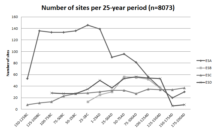
Figure 1. The number of sites each ware is attested at per 25-year period (data from the ICRATES database, \(n=8073\) tableware sherds). This figure illustrates that ESA is attested on far more sites than the other three wares for the period of 150BC-75AD. - 2.3
- Archaeologists and historians have argued over a wide range of different conceptual models to explain this pattern in the tableware distribution (e.g. Abadie-Reynal 1989; Bang 2008; Bes 2015; Lewit 2011; Reynolds 1995). Although each author argues the Roman trade system was a complex system and agrees it consisted of a combination of driving forces, each author places an emphasis on different factors (e.g. state involvement, redistributive centres, consumption "pulling forces", commercial "piggy-back" trade, closeness to large-scale agricultural production). However, the ability to compare different models in a strictly conceptual way, as thought-experiments, is limited due to a number of issues. Firstly, the existing conceptual models rarely abstract the complex past phenomenon that is the Roman trade system in terms of concepts more commonly used in economics or other disciplines that would facilitate comparison, or commonly used concepts and how these can be identified in the available sources are defined differently by different authors. Secondly, specifications for the kinds of data patterns one would expect to see as an outcome of different conceptual models (i.e. model predictions) are rarely provided.
- 2.4
- To illustrate these issues and the potential of computational modelling for the study of the Roman economy, we will focus here on two conflicting conceptual models: Peter Bang's Roman bazaar (2008) and Peter Temin's Roman market economy (2013). Here we will focus in particular on the elements of these models that concern the flow of commercial information between traders. Bang suggests the Roman Bazaar concept to describe such flows: local markets distinguished by high uncertainty of information; relative unpredictability of supply and demand; communities of traders active on different markets were opportunistic and protectionist. In Bang's conceptualisation all of these factors led to poorly integrated markets throughout the empire characterised by a limited availability of commercial information between markets. Temin agrees with Bang that the information available to individuals was limited and that local markets are key structuring factors. However, contrary to Bang he believes that the Roman economy was a well-functioning integrated market where prices are determined by supply and demand. A key difference between both models is the degree of market integration, which represents the availability of commercial information (supply, demand, prices) to traders on different markets. Bang argues that different circuits for the flow of goods could emerge as the result of different circuits for the flow of commercial information. In other words, the observed distribution patterns of wares are a reflection of the functioning of past social networks between traders on different markets (Bang 2008, 288). Temin's model can be considered to offer an alternative, where the structure of social networks as a channel for the flow of commercial information must have enabled strongly integrated markets.
Model
description
- 3.1
- We will first present a summary overview of the workings of the model. This will be followed by a description of how the conceptual models by Bang and Temin are abstracted using a conceptualisation that allows for comparisons between both, and how this conceptualisation is represented in MERCURY. We will then provide a technical description of the procedures used to initialise the model, and of the trade procedures used when the model is running. Finally, the design of the presented experiments and the selected parameter ranges are discussed. Variable names used in the model are in italics. Table 1 lists all independent and dependent variables included in this ABM with a short description and their tested or default value (excluding reporter and counter variables which are listed in Supplement 2).
- 3.2
- These conceptualisations, representations, and procedures
are implemented in an ABM coded in Netlogo v.5.0.5 using the 'network'
and 'nw' extensions.[1]
MERCURY and its documentation following the ODD (Overview, Design
concepts, Details) protocol (Grimm et
al. 2006; 2010)
can be downloaded from the OpenABM repository (Brughmans & Poblome 2015).
Model overview
- 3.3
- The MERCURY model represents the structure of social
networks between traders that act as the channels for the flow of
commercial information and goods. The model is initialised by creating
a social network between traders who are distributed among sites. Four
of these sites are production centres. Each of them produces one of the
four different wares, and traders located at these sites obtain a
number of items of this locally produced ware in each turn. At each
time step traders will determine the local demand for tableware they
want to satisfy, and will estimate the price they believe an item of
tableware is worth based on their knowledge of the supply and demand of
the traders they are connected to. Every item of tableware is then put
up for sale, and pairs of traders who are connected in the network can
buy or sell an item. When an item is successfully traded, the buyer
will decide to either sell it to a local consumer to lower the demand
(in which case the item is taken out of the trade system and is
deposited at that site), or to store it for redistribution in the
following turn in case this promises a higher profit. Over time, this
model therefore gives rise to distributions of four tablewares which
can be compared to the archaeological data.
Conceptualisation and representation
- 3.4
- The social networks described by Bang consist of a strong community
structure within markets, limited
availability of commercial information between communities,
and weakly integrated markets. The system described
by Temin consists of limited availability of commercial
information, and well integrated markets
where prices are determined by supply and demand.
The terms in bold are concepts these authors use to abstract their
ideas about Roman trade, and need to be clearly defined before their
implementation in computer code. The social network aspects of the
models by Bang and Temin can be usefully conceptualised and represented
as follows (the most fundamental concepts are introduced first,
followed by more elaborate concepts that build on the definitions of
the fundamental concepts):
- Commercial actors.
Conceptualisation: these have agency and are here referred to as traders. No differentiation is made between types of traders, other than the ability to trade within a market and/or between markets, depending on the network neighbours of the trader.
Representation: software agents represented as nodes. - Markets.
Conceptualisation: places where traders come together, where different communities of traders exist, and where tableware and commercial information are available. We decided to use the archaeological term "sites" in this paper and in the ABM code to refer to our representation of the markets discussed by Bang and Temin, for two reasons: to avoid equating the past phenomenon under study (the Roman market economy) with the approach (ABM) and data (archaeological finds) we use to study it; and to facilitate comparison between the simulated distributions and the archaeologically observed pottery distributions (referred to by archaeologists as the assemblages excavated at sites).
Representation: a location in abstract space on which a set of traders is located. All traders are distributed among all sites. Tableware is deposited on sites through trade procedures, and these simulated deposits can be compared to excavated deposits at archaeological sites. - Product.
Conceptualisation: one of four tablewares.
Representation: four tablewares are here referred to as four products (A, B, C, D). Each product is produced at a different site. Units of each product are exchanged between traders through trade, and are deposited at sites. Each product is valued equally by traders, since we assume consumers obtain tableware for functional rather than aesthetic or other purposes. MERCURY is not designed to test alternative valuations. - Supply.
Conceptualisation: the amount of tableware a trader owns and is willing to sell.
Representation: the amount of tableware each trader owns at the start of each time step. - Demand.
Conceptualisation: here used as the demand for tablewares of consumers at a site a trader is aware of and is able to supply for.
Representation: Demand is a variable of traders. Demand can only be satisfied by obtaining an item of any product through a successful transaction between a pair of traders. It is assumed here that each trader has the ability to supply at most for a fixed maximum demand in each time step, determined by the independent variable max-demand. MERCURY is not designed to test traders with variable abilities to satisfy demand. - Commercial information.
Conceptualisation: the knowledge a trader obtains of supply and demand.
Representation: traders obtain the values of supply and demand from a proportion of the traders they are connected to and use it to estimate the price they believe tableware is worth within their part of the social network. - Social network.
Conceptualisation: traders have the ability to share commercial information and tableware with other traders they are directly connected to in a social network.
Representation: a non-directed edge between a pair of nodes represents the ability to share tableware and commercial information between this pair of nodes. The set of all nodes and the set of all edges constitute the social network. - Limited availability of information.
Conceptualisation: only a proportion of the traders a trader is able to trade with shares commercial information with that trader.
Representation: the proportion of a node's neighbouring nodes in the social network of which it knows the supply and demand. The variable local-knowledge is used to implement this proportion in the code, one of the dependent variables of the model tested in experiments. A low value of this variable represents limited availability of accurate commercial information (as both Bang and Temin argues was the case in the Roman trade system). - Community structure.
Conceptualisation: communities consist of traders who are more likely to trade and share commercial information with each other.
Representation: a social network structure with a high clustering coefficient within sites, and with a lower number of links between clusters than within clusters. In other words, the social network of traders within each site will have a 'small-world' network structure with a high clustering coefficient and a low average shortest path length (Watts & Strogatz 1998). - Market integration
Conceptualisation: the ability to share commercial information and goods between markets.
Representation: the proportion of all possible edges between nodes that connect nodes on different sites. This proportion is tested by varying the variable proportion-inter-site-links in experiments. A high value for this variable represents highly integrated markets (as suggested by Temin), a low value represents weakly integrated markets (as suggested by Bang).
- Commercial actors.
- 3.5
- A final important factor is the conceptualisation of time
in the model. In archaeology, the accuracy of dates is often
problematic. The lower and upper limits of how long an item of
tableware remained in use vary greatly, as shown by Peña (2007) in his model of the
use-life of this type of pottery. Moreover, as illustrated by Willet's (2012, 44–46) calculation, these
are only estimates and they suggest extreme differences in the volumes
of tableware in circulation in the Eastern Mediterranean during the
study period. In this model we therefore decided to work with a
relative 'transaction time' rather than an absolute timeframe: the time
of each time step is the time it takes for all tableware available for
trade to be considered in a transaction, and the demand to increase by
one item per trader if it is not at its maximum.
Initialization procedures
- 3.6
- The model is initialized in three steps, in this order:
creating sites and traders, distributing the traders among the sites,
and connecting traders in a network (Figure 4
presents a flowchart of the initialization).
Creating sites and traders
- 3.7
- A set of sites and a set of traders are created determined
by the variables num-sites and num-traders
respectively. The numbers of sites and traders do not
change throughout an experiment. Sites are positioned in a circular
layout, which is convenient for setting up the social network and for
visualisation, but the network is the only means of determining
proximity between sites. The model is not spatial as it does not
represent the geographical distribution of sites. Four sites, equally
spaced along the circle, are selected to become production sites of one
of four products each.
Distributing traders
- 3.8
- When equal-traders-production-site is set to 'true', an equal number of traders (determined by the variable traders-production-site) is moved to each production site. The remaining traders are then distributed on the other sites following a uniform or exponential frequency distribution, depending on the setting of the variable traders-distribution.
- 3.9
- When equal-traders-production-site is set to 'false', all traders are distributed among all sites (i.e. including the production sites) following a uniform or exponential frequency distribution, depending on the setting of the variable traders-distribution.
- 3.10
- The mean of the exponential frequency distribution is the number of traders that have not yet been moved to a site divided by the number of sites.
- 3.11
- The exponential frequency distribution will result in
strong differences between the number of traders per site, where a few
sites have a very high number of traders and most sites have a much
lower number of traders. Since the maximum demand of a site in this
model is determined by the number of traders present at a site, this
exponential distribution of traders is considered to reflect the
differing demands of markets throughout the Mediterranean: markets with
an extremely high demand are relatively rare (e.g. in the cities of
Alexandria, Antioch, Ephesos) whilst most markets will have a much more
modest demand. A uniform frequency distribution of traders is
considered unrealistic, but is included as a benchmark to compare its
outputs with that of experiments with an exponential frequency
distribution.
Creating the social network
- 3.12
- Traders are subsequently connected to each other to form a
social network with a structure that represents the hypotheses tested
by setting the variable network-structure to the
value "hypothesis" (this variable can also be set to "random" in order
to compare the results of experiments to those of an experiment with a
graph created through a random process with the same density). This
hypothesised structure, as mentioned above in section
Conceptualisation and repesentation
is considered to have a high
clustering coefficient within sites, relatively few links between
clusters within sites, and a modifiable proportion of links between
sites. It was decided to use the 'small-world' network structure as a
baseline for creating this hypothesised network within sites, and to
combine this with a variable that allows for modifying the proportion
of links between sites (proportion-inter-site-links).
The procedures to create a social network in MERCURY are based on the
initialisation procedures of the model for the growth of social
networks with a 'small-world' structure by Jin, Girvan and Newman (2001; referred to in Jin et al.
2001 as Model II), which has previously been applied in an
archaeological model of exchange by Bentley, Lake and Shennan (2005). The simplified version
of the model was selected because it gives rise to the network
structure of interest (maximum degree, low average shortest-path
length, high clustering coefficient) with relatively few parameters.
MERCURY's network creation procedures consist of five steps (see Fig. 2;
Supplement 1 includes the number
of edges created in each of these five steps for each experiment):
- Firstly (Fig. 2a), between each pair of neighbouring sites on the circular layout, one pair of randomly selected traders located on neighbouring sites is connected. This ensures a minimum of connectivity between sites that allows for goods to still be distributed to all sites. In scenarios where no other inter-site links are added, information and goods will therefore need to travel from site to site along the circular layout.
- Secondly (Fig. 2b),
a number of inter-site links is created. A proportion (determined by
the variable proportion-inter-site-links) of all
trader pairs are connected if a pair is not located on the same site
and is not connected yet. The total number of trader pairs is
calculated as:
Calculation of total number of trader pairs:
$$ \frac{1}{2} N (N-1)$$(1) - Steps three and four will result in a 'small-world' network structure within sites, where clusters exist that have few connections between clusters. These steps are adopted from the model by Jin et al. (2001). Thirdly (Fig. 2c), randomly selected pairs of traders on the same site are connected. More formally, a proportion of all trader pairs determined by the variable proportion-intra-site-links are connected if they meet the following requirements: both are located at the same site, the pair is not connected yet, and neither of the traders has the maximum-degree.
- Fourthly (Fig. 2d),
pairs of traders on the same site with a mutual neighbour in the
network will be connected. This step is responsible for the high level
of clustering and is a process common in social networks called
transitivity, which stands for the idea that a pair of individuals who
have a mutual friend have a high probability of becoming friends
themselves in the future. The step is implemented as follows: a number
of traders are selected uniformly at random; the number of selected
traders is a proportion of all trader pairs with a mutual neighbour
(the proportion is determined by the variable proportion-mutual-neighbors,
and the number of trader pairs with a mutual neighbour is calculated as
in eq. 2); if these randomly selected traders are connected to a pair
of traders on the same site that are not connected yet and do not have
the maximum-degree, then such a pair of traders of
whom the randomly selected trader is a mutual neighbour will be
connected. Equation 2 shows the calculation of all trader pairs with a
mutual neighbour:
Calculation of all trader pairs with a mutual neighbour:
$$\frac{1}{2} \sum_{i} z_i (z_i-1)$$(2) - Fifthly (Fig. 2e), at this stage the network can still consist of multiple components, i.e. there exist subsets of nodes, where nodes within subsets can be connected but there are no edges between the subsets. This would prohibit tableware produced in one area of the network to reach traders in another. Therefore, a minimum number of edges are added between pairs of traders on the same site which are not in the same component, to ensure all traders become part of a single component. This generally results in very few extra links being created (between 2 and 19 in the experiments presented here) and has a minimal impact on the 'small-world' structure of the networks within sites.
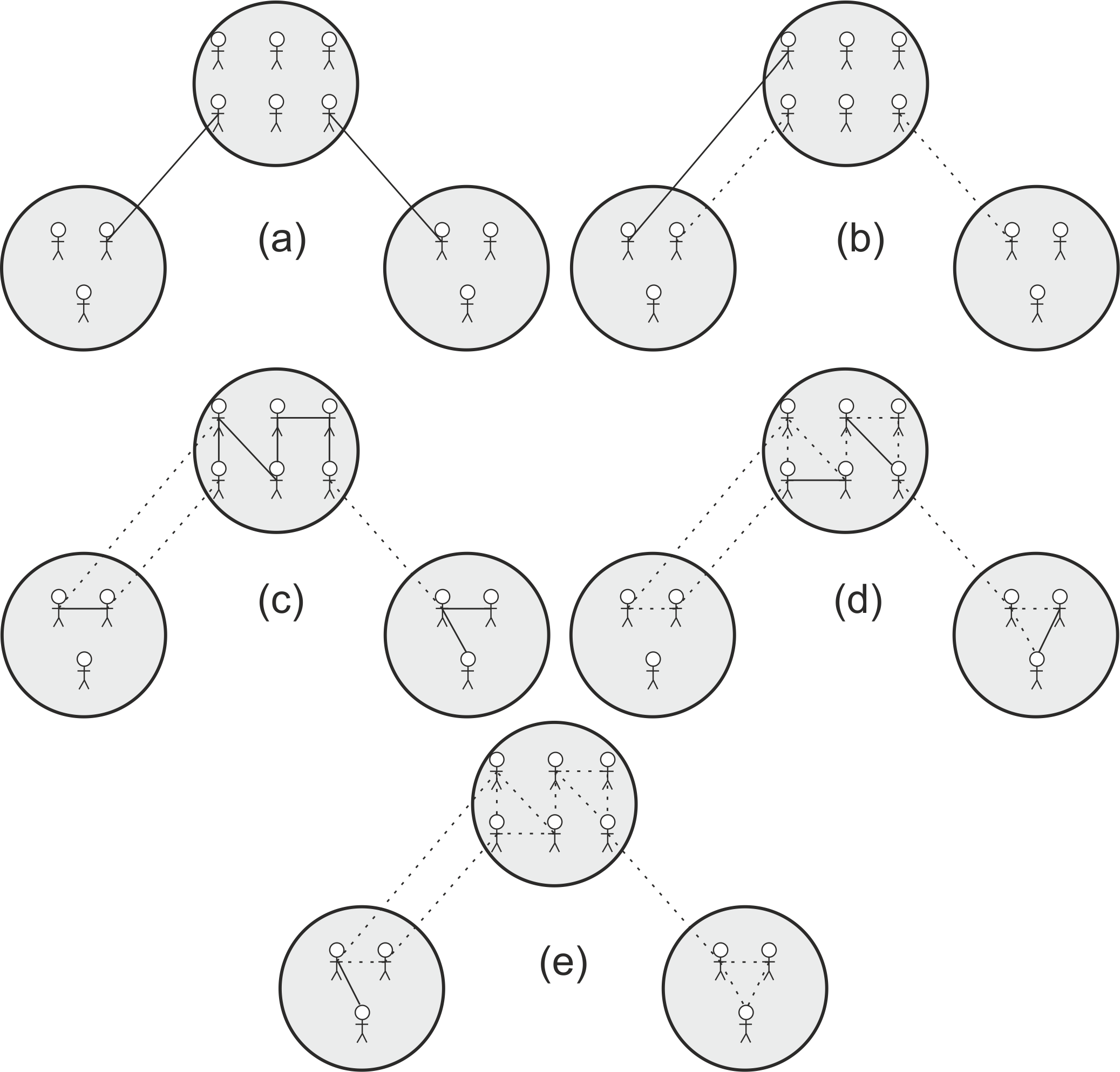
Figure 2. Abstract representation of the five-step procedure (a-e) used to create the hypothesised network structure. Traders are represented as stick figures and are distributed among sites represented as circles. Newly created edges are represented as solid lines, dashed lines represent existing edges. (a) a pair of traders on each pair of neighbouring sites is connected; (b) randomly selected pairs of traders on different sites are connected; (c) randomly selected pairs of traders on the same site are connected; (d) pairs of traders on the same site with a mutual neighbour are connected; (c) and (d) are repeated until all or most traders have the maximum allowed number of connections; (e) a minimal number of randomly selected traders in different components on the same site are connected. Note the final network structure (e) consists of clusters of traders on sites, a limited number of edges between clusters, a proportion of edges between traders on different sites, and a single connected component. - 3.13
- The result is a network structure where neighbouring sites
are connected by at least one edge between a pair of traders, where
traders within the same site are connected in clusters with few
connections crossing clusters, and with a variable number of inter-site
links depending on whether Bang's or Temin's hypothesis is being tested
(Fig. 3), and all traders being
part of a single connected component. Traders on each site are
therefore connected following a 'small-world' network structure (Watts
and Strogatz 1998), with a high clustering coefficient and a
low
average shortest path length. However, the overall network structure of
all traders on all sites combined will not always show the
characteristics of a 'small-world' network, since the number of
inter-site edges added in addition to the edges connecting traders on
neighbouring sites is determined by the variable proportion-inter-site-links
used to represent different degrees of integration of markets (see
Supplement 1).
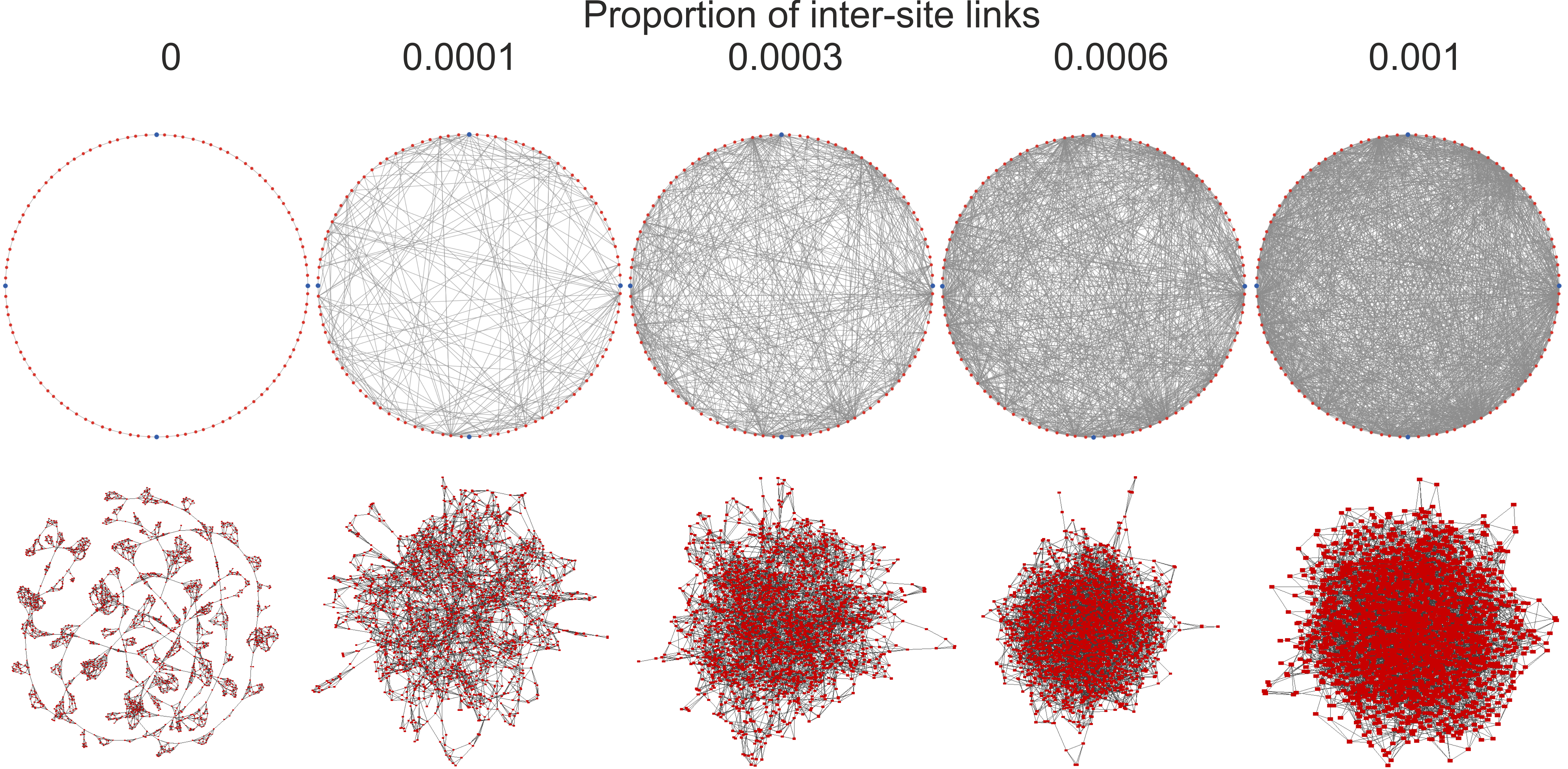
Figure 3. Example of the network structure generated in the setup procedure of MERCURY showing the resulting networks for different values of the proportion-inter-site-links variable. The top row shows a network of sites layed-out along a circle with traders positioned at sites. The bottom row shows the same networks but nodes now represent traders and the traders' social network laid-out using a force-directed layout algorithm (yFiles Organic layout in the network science software Cytoscape) to display its structure. Note the existence of clusters of traders on sites connected to few other clusters when the proportion of inter-site links is low (extreme left), a pattern which gradually disappears as traders receive more inter-site links and the sites become more integrated. 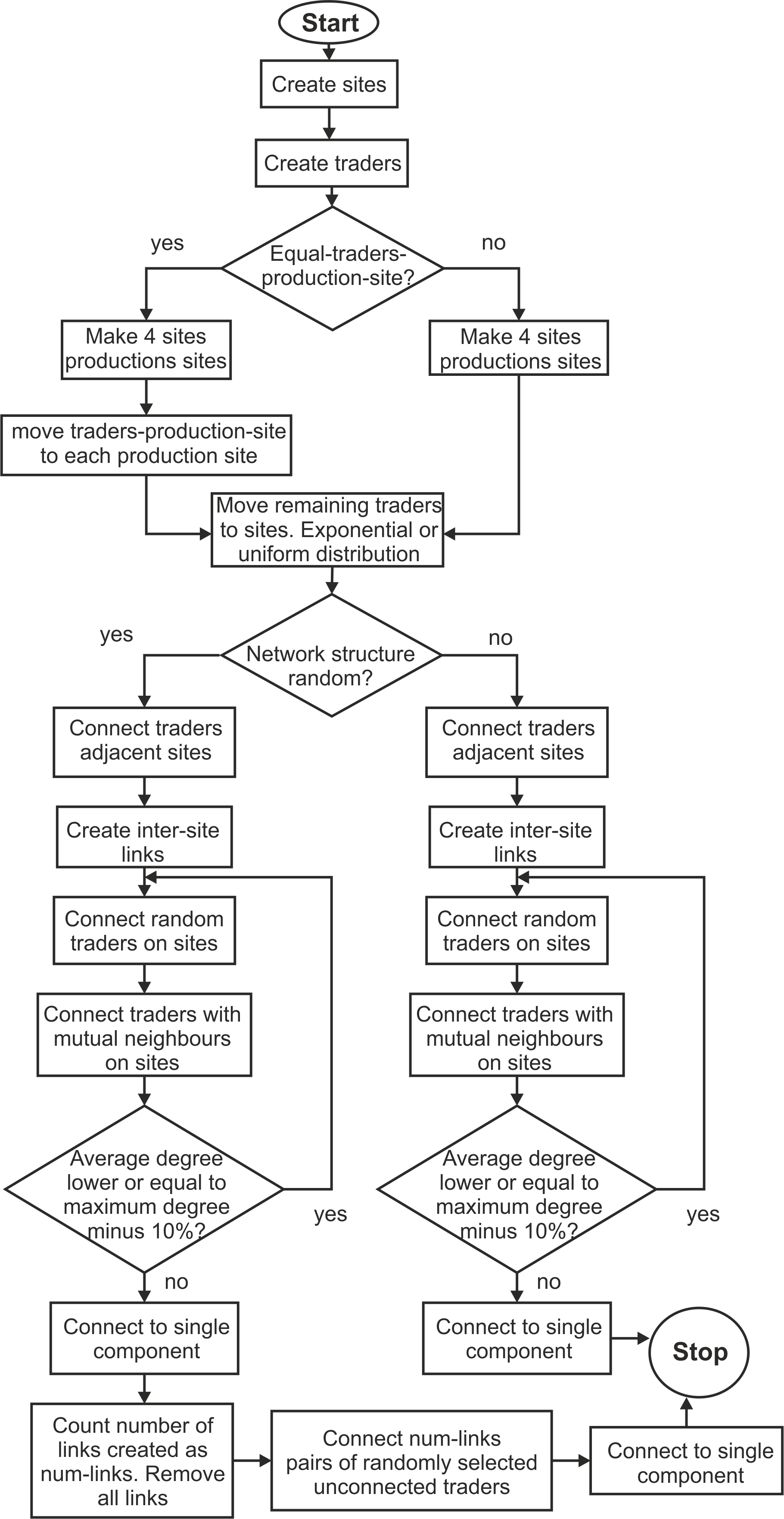
Figure 4. Flowchart of initialization procedures in MERCURY. Trade procedures
- 3.14
- In every time step of the model the trade procedures follow
these steps: 1) all traders determine demand, 2) they discard part of
their stock, 3) traders on tableware production sites obtain new items,
4) all traders obtain commercial information, 5) they determine what
they believe to be the current price for a tableware item, 6) they
determine the maximum amount of items they are willing to stock in that
time step, and finally 7) all items owned by all traders and not in
stock are traded. Each step will be described in detail in the next
subsections (Figure 5 presents
a flowchart of the trade procedures).
Determining demand
- 3.15
- The demand of each trader is 0 at the
start of the simulation. At each time step, a traders' demand
is increased by 1 if his demand is lower than the
trader's maximum demand determined by the independent variable max-demand.
In other words, when a consumer obtains an item they do not immediately
require a new one and at some point the inhabitants of a site do not
require any more tableware. Instead, the demand gradually increases to
the maximum. This mirrors the background microprocesses of losing, or
breaking an item of tableware, of items becoming unfashionable with
time, or any other microprocesses that result in the renewed need for
the item. The total demand at sites will therefore reflect the
distribution of traders among sites: the summed maximum demand per site
will be equal for all sites in case of a uniform distribution of
traders among sites, and will show strong differences in case of an
exponential distribution of traders among sites. However, the total sum
of maximum demand in the model for experiments with the same number of
traders will always be the same, which facilitates comparison of
experiment results.
Discard part of stock
- 3.16
- The ability for goods to be redistributed is key in both
Bang's and Temin's conceptual models of the Roman trade system and is
implemented in MERCURY by allowing traders to stock products. In the
previous time step products can be put in stock as a result of either a
failed transaction or a deliberate storing of the item for
redistribution in the next turn (see Trade
products below). At the start of a
time step traders who have stock will need to discard a fixed
proportion of it. This penalty reflects the risks involved in not
immediately selling an item on to a consumer but storing it for
redistribution and represents broken or unfashionable items. The
remainder of the stock is then considered for trade in the rest of this
time step. The proportion of discarded items is set to 14%, which is a
proportion suggested by Peña's (2007,
Fig. 11.5) model for the life cycle of tableware distributed beyond the
local area of its manufacture.
Production
- 3.17
- Traders located on sites that were selected in the setup
procedures as the production sites will obtain newly produced items
each time step, only if their total current possession of all four
products is less than their demand. If this is the
case then they obtain items of the product being produced at that site
equal to their demand minus the sum of the products
they already possess, i.e. they obtain the number of items needed to
reach their demand.
Obtaining commercial information and price-setting
- 3.18
- Once every time step, and before trade happens, a
proportion of a trader's neighbours in the social network will be
randomly selected as the trader's informants. From this proportion of
neighbours the trader will know the demand and the
sum of all items of all products they own (i.e. their supply). This
proportion is determined by the independent variable local-knowledge
and is used in the experiments to test scenarios with differing
availability of information (together with the proportion-inter-site-links
variable). The trader then calculates the average demand and average
supply of this proportion of neighbours, including his own supply and
demand. Using this commercial information available to him he then
determines what he believes is the price of one item of any product as
follows:
$$ price = \frac{average~demand}{average~supply + average~demand} $$ (3) - 3.19
- This results in a float value normalised between 0 and 1
following the logic of supply and demand: if the average demand is
equal to the average supply then the price will be 0.5; if the average
demand is higher than the average supply then the price will be between
0.5 and 1; if the average demand is lower than the average supply then
the price will be between 0 and 0.5.
Determine maximum stock
- 3.20
- The traders will subsequently determine how many items they
are happy to store for redistribution in the next turn. For each trader
the maximum-stock-size dependent variable is
calculated as the average of the demand of the
other traders he knows commercial information of, minus his own demand,
rounded. The maximum stock is only higher than 0 when the average demand
is higher than his own demand, i.e. when the trader
believes there is a high demand which promises
higher profits (because his own demand is lower) he
will be willing to store the number of items necessary to supply for
the average demand.
Trade products
- 3.21
- Each item of every product is considered for trade once per time step. A single item is selected at random and the trader who owns it will consider selling it individually. An item is put in the trader's stock if he cannot make a profit or if none of his neighbours in the network require an item (i.e. their demand equals 0). An item is sold to a buyer if the buyer's price offers a profit or break-even for the seller. A seller will therefore only agree to sell tableware for more or the exact amount he estimates it is worth, and a buyer will only buy tableware for less or the exact amount he estimates it is worth (this means that there is no formal procedures for negotiation of prices and market clearance, a simplification introduced because MERCURY is designed only to evaluate the impact of differential availability of commercial information).
- 3.22
- The buyer either places the obtained item in stock for redistribution if the average demand is higher than his demand (i.e. redistribution holds the promise of a higher profit), or if this is not the case he deposits it on his site (this action represents the trader selling the item to a consumer and the item leaving the trade cycle). In the latter case the buyer's demand is decreased by 1 because some of the local consumers' demand is satisfied; the item is taken out of the trade system because the consumer does not redistribute it; and it is deposited on the buyer's site (the site's dependent variable for that product (volume-A, -B, -C, or –D), is increased by 1).
- 3.23
- This sequence of procedures results in distribution of four
different products representing tablewares on sites. The volume and
diversity of tableware deposited on sites can subsequently be used to
compare the simulated tableware distribution with the archaeologically
attested one (see Brughmans
& Poblome 2016).
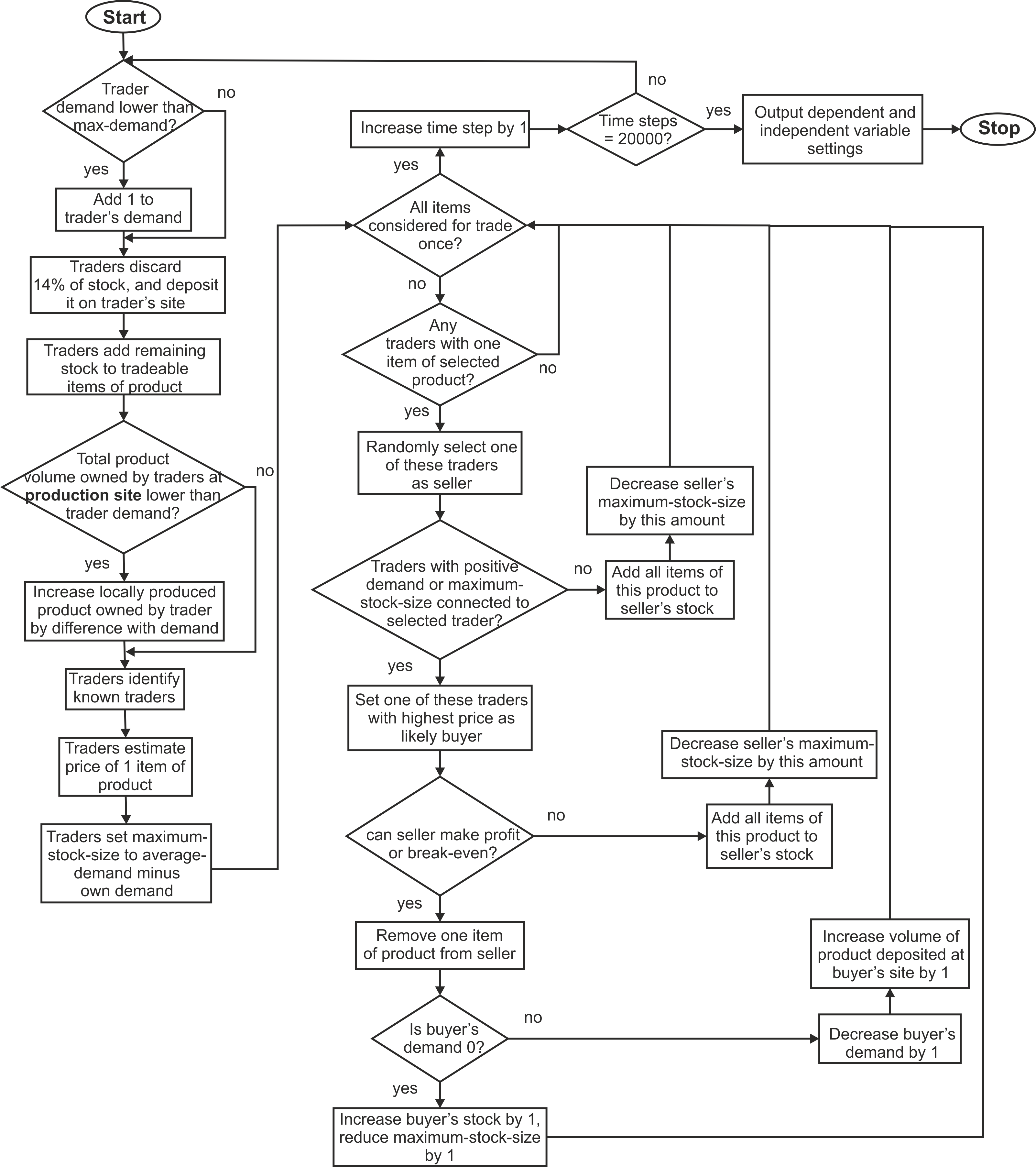
Figure 5. Flowchart of trade procedures in MERCURY. Experiments and variable settings
- 3.24
- MERCURY allows us to compare and provide predictions for
the conceptual models of Bang and Temin by changing the degree of
market integration (i.e. the proportion of edges between traders
located on different sites, controlled by the proportion-inter-site-links
variable) and by changing the availability of commercial
information (controlled by the local-knowledge and
proportion-inter-site-links variables). A
number of other independent variables are changed in separate
experiments to explore different social network structures and trade
procedures.
Supplement 1 lists each experiment's settings for the
independent variables, summary network measures for the resulting
network structure, and summary statistics for the simulated
distribution of products. Experiments were designed to explore the
effects of changing the following independent variables:
- Changing the proportion of all trader pairs that are connected and are not located on the same site from 0%, to 0.01%, 0.06%, 0.1%, 0.2% and 0.3% (i.e. changing the proportion-inter-site-links variable);
- changing the proportion of neighbours a trader can obtain commercial information from between 10%, 50% and 100% (i.e. changing the local-knowledge variable);
- replacing the hypothesised social network structure with a randomly created network structure with the same density (i.e. changing the network-structure variable);
- varying the number of traders located at production sites in a range between 1 and 30 (i.e. changing the traders-production-site variable);
- changing the distribution of all traders at all sites between uniform and exponential (i.e. changing the traders-distribution variable);
- varying the maximum demand of traders in a range between 1 and 30 (i.e. changing the max-demand variable).
- 3.25
- In these experiments, the independent variables listed in
Table 1 are hypothesised to
cause the differences in the volume and diversity of products deposited
at sites (dependent variables), and once their values are set during
the initialisation of the model they will not change during an
experiment. The dependent variables (Table 1)
dynamically change throughout the simulation as a result of the
simulated trade procedures. The model outputs are the values of the
dependent variables at the end of an experiment, i.e. the simulated
volume of each tableware at sites. The output allows us to derive the
diversity of products at sites and the wideness of products'
distributions. The latter output in particular can be compared with the
distributions of tablewares in archaeological datasets. The default
values used in the experiments presented here for a number of
independent variables are further discussed in
Supplement 2. Each
experiment was run for 20,000 time steps, a decision made in the
absence of a realistic conceptualisation of time as described above,
motivated by the observation that the wideness of wares' distributions
(the pattern of interest in this study) stabilises the first 5000 time
steps, and remains more or less fixed for the remaining time.
Table 1: Independent and dependent variables used in MERCURY, with a short description and the values used in experiments. See Supplement 2 for a similar list which additionally includes all counter and reporter variables, and a motivation for the selection of a default value in experiments for a number of independent variables. Independent variables Variable Description Tested values Global variables num-traders The total number of traders to be distributed among all sites 1000 num-sites The total number of sites 100 equal-traders-production-site Determines whether the number of traders at production sites will be equal and determined by the variable 'traders-production-site' or whether it will follow the same frequency distribution as all other sites determined by the variable 'traders-distribution' true, false traders-distribution Determines how the traders are distributed among the sites exponential, uniform traders-production-site Determines the number of traders located at production sites if 'equal-traders-production-site' is set to 'true' 1, 10, 20, 30 network-structure Determines how the social network is created when initialising an experiment: a randomly created network, or the network structure hypothesised by Bang or Temin. hypothesis, random maximum-degree The maximum number of connections any single trader can have 5 proportion-inter-site-links The proportion of all pairs of traders that are connected in step two of the network creation procedure by inter-site links 0, 0.0001, 0.0006, 0.001, 0.002, 0.003 proportion-intra-site-links The proportion of all pairs of traders that are considered in step three of the network creation procedure to become connected by intra-site links 0.0005 proportion-mutual-neighbors The proportion of all pairs of traders with a mutual neighbour that are considered for becoming connected in step four of the network creation procedure by intra-site-links 2 Site-specific variables production-site Set to "true" if the site is a production centre of one of the products true, false producer-A Set to "true" if the site is the production centre of product-A true, false producer-B Set to "true" if the site is the production centre of product-B true, false producer-C Set to "true" if the site is the production centre of product-C true, false producer-D Set to "true" if the site is the production centre of product-D true, false Trader-specific variables max-demand The maximum demand each trader aims to satisfy 1, 10, 20, 30 local-knowledge The proportion of all link neighbours a trader receives commercial information from (supply and demand) in each turn 0.1, 0.5, 1 Dependent variables
Variable Description Site-specific variables volume-A The number of items of product A deposited on the site as a result of a successful transaction volume-B The number of items of product B deposited on the site as a result of a successful transaction volume-C The number of items of product C deposited on the site as a result of a successful transaction volume-D The number of items of product D deposited on the site as a result of a successful transaction Trader-specific variables product-A The number of items of product A the trader owns and can trade or store in this turn product-B The number of items of product B the trader owns and can trade or store in this turn product-C The number of items of product C the trader owns and can trade or store in this turn product-D The number of items of product D the trader owns and can trade or store in this turn stock-A The number of items of product A the trader puts in his stock in this turn as a result of an unsuccessful transaction or for redistribution in the next turn stock-B The number of items of product B the trader puts in his stock in this turn as a result of an unsuccessful transaction or for redistribution in the next turn stock-C The number of items of product C the trader puts in his stock in this turn as a result of an unsuccessful transaction or for redistribution in the next turn stock-D The number of items of product D the trader puts in his stock in this turn as a result of an unsuccessful transaction or for redistribution in the next turn maximum-stock-size The number of items the trader is willing to obtain through trade this turn in addition to his own demand if the average demand is higher than his demand price The price the trader believes an item is worth based on his knowledge of supply and demand on the market demand The proportion of the demand at the market the trader is located at that he aims to satisfy by obtaining products through trade. Constant increase of 1 per turn; maximum = max-demand
Results
- 4.1
- As discussed in the introduction, the research question
that motivated the creation of MERCURY is: under what conditions does
the model give rise to one product being much more widely distributed
than the three other products? This pattern is here studied through two
measures: the number of sites at which each of the four products was
deposited in experiments (referred to as the width of a product's
distribution), and the maximum number of sites a ware is deposited on
minus the minimum number of sites another ware is deposited on per
iteration of each experiment (referred to as the range of
distribution). In order to assess whether an experiment approximates
the pattern observed in the archaeological record we evaluate whether
it shows a high range of distribution and whether on average one
product has a higher width than others, i.e. one product is deposited
on far more sites than others.
Number of edges
- 4.2
- The setup procedure of MERCURY results in a static network structure with different proportions of edges between traders located on different sites depending on the setting of the proportion-inter-site-links variable. However, the total number of edges is similar in all experiments, with small variations due to the stochasticity (built-in randomness, see the ODD for a list of stochastic processes) in the model (Table 2, see also Supplement 1 for all experiments). Thus an increased proportion of inter-site edges results in a lower number of randomly created intra-site edges (step 3) and, in particular, intra-site edges between traders with a mutual neighbour (step 4). The latter is caused by the decreasing number of trader pairs on sites that have a mutual neighbour as the value of proportion-inter-site-links is increased. The tested values for proportion-inter-site-links range from 0%, to 0.01%, 0.06%, 0.1%, 0.2% and 0.3% of all trader pairs (see Table 2, in grey and underlined), resulting in almost no market integration to 100% market integration where all links are between trader pairs on different sites (see Table 2, in bold and underlined). These different degrees of market integration strongly affect the overall structure of the network as shown by the network measures in Table 2: both the clustering coefficient and the average shortest path length decrease considerably with an increase in market integration.
- 4.3
- The social networks created in MERCURY are therefore very
different depending on the degree of market integration selected in
experiments: in scenarios with low market integration there will be
strong clustering within markets (representing communities) but the
shortest paths between trader pairs will be long (e.g. experiment 1)
representing the conceptual model of Bang. On the other hand, in
scenarios with high market integration there will be very limited
clustering within markets but short paths between all trader pairs as
proposed by Temin. A graph created through a random process with the
same density (i.e. number of edges divided by the number of traders)
and consisting of one connected component represents almost no
clustering within markets and almost complete market integration (e.g.
experiment 35).
Table 2: The number of edges created in each step of the setup procedure for selected experiments representing different degrees of market integration (i.e. different values for the variable proportion-inter-site-links in grey and underlined). The total proportion of inter-site edges is the sum of steps 1 and 2 divided by the total number of edges in the network, results are shown in bold and underlined. Some variable settings for experiment 35 are presented in brackets, because in this experiment a randomly created network is considered with the same number of edges as the equivalent hypothesised network structure with the same variable settings. (exp. = exponential, hypo. = hypothesis). 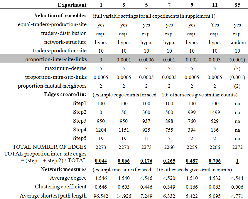
Effects of proportion-inter-site-links and local-knowledge
- 4.4
- The proportion of commercial information available to
traders has a limited effect on the wideness of the distribution of
products. Experiments where traders have access to the commercial
information of 10% of the traders they are connected to show only
slightly more widely distributed products than those where traders have
access to information from 100% of their contacts (i.e. changing the local-knowledge
variable between 0.1 and 1; Table 3).
A higher integration of markets (i.e. a higher value for proportion-inter-site-links)
does give rise to more widely distributed products. Despite this wide
distribution of products, the range of their distribution (i.e. the
difference between the maximum and minimum wideness of four products'
distributions per simulation) is rather low. These results suggest that
the impact of the local-knowledge variable on the
wideness of distribution is limited, and that a high degree of market
integration as represented by a high value for proportion-inter-site-links
can give rise to widely distributed products but that it
is not sufficient for explaining the differences in the width of
products' distributions.
Table 3: Selected variable settings and summary results for experiments designed to evaluate the effects of two independent variables: proportion-inter-site-links and local-knowledge. The following describes the information presented in Tables 3, 4, 5 and 6. Results are highlighted using a colour range from light grey for 0 and dark grey for 100 (the minimum and maximum widths of distributions in these experiments). 'Ranked width distributions' presents the number of sites each product is deposited on, averaged over 100 iterations per experiment (seed 1-100). Results for the most widely distributed wares in all iterations of an experiment were averaged and reported as 'Product 1', results for the second most widely distributed products as 'product 2', etc. 'Range of distributions' presents summary statistics of the difference in distribution width between product 1 and product 4 for all iterations per experiment. See Supplement 1 for a full list of experiments with their variable settings and summary results. 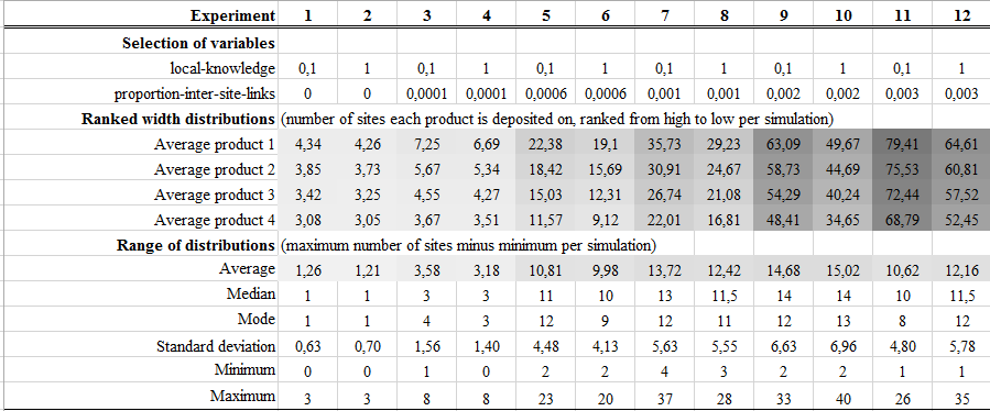
Effects of traders-production-site and max-demand
- 4.5
- The results of experiments 13 to 20 presented in Table 4 show the distribution of products
in scenarios where an equal number of traders are present on each of
the four production sites, determined by the variable traders-production-site,
and the rest of the traders are distributed exponentially among the
remaining sites, determined by the variable traders-distribution.
Increasing either or both the traders-production-site
and max-demand variables results in more widely
distributed products (i.e. higher width of distributions for products
1, 2, 3, and 4), but does not lead to very strong differences between
the width of products' distributions (i.e. limited ranges of
distributions).
Table 4: Selected variable settings and summary results for experiments designed to evaluate the effects of two independent variables: traders-production-site and max-demand. See caption Table 3 for a detailed description of the information presented in this table. 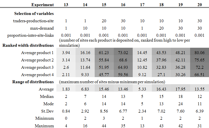
Effects of traders-distribution and equal-traders-production-site
- 4.6
- The results of the experiments presented in Table 5 are the outputs of scenarios
where the number of traders at the four production sites are unequal
and follow the exponential or uniform (determined by the variable traders-distribution)
distribution of all traders among all sites. We notice that an overall
exponential distribution of traders on all sites in a scenario with
limited market integration does not give rise to widely distributed
products and high ranges of distribution (see experiment 21). However,
increasing the degree of market integration (by increasing the proportion-inter-site-links
variable) does result in more widely distributed products
and higher ranges of distribution (see experiments 24-28). Moreover,
when one production site has far more traders than any of the others,
the product produced at this site will be far more widely distributed
than the others (see experiment 33). We again notice that, even with an
unequal number of traders at production sites, a local-knowledge
value of 0.5 results in slightly more widely distributed products and
slightly higher ranges of distribution than a value of 1, as mentioned
in section 'Effects of proportion-inter-site-links and
local-knowledge' above (compare experiments 24
and 31). A uniform distribution of all traders among all sites results
in wide distributions of products, but also a low range of distribution
(see experiment 23).
Table 5: . Selected variable settings and summary results for experiments designed to evaluate the effects of two independent variables: equal-traders-production-site and traders-distribution. The setting for traders-production-site for experiment 33 is given in brackets, because in each iteration of this experiment the number of traders at production sites A, B, C, and D was set to 30, 1, 1, and 1 respectively. See caption Table 3 for a detailed description of the information presented in this table. 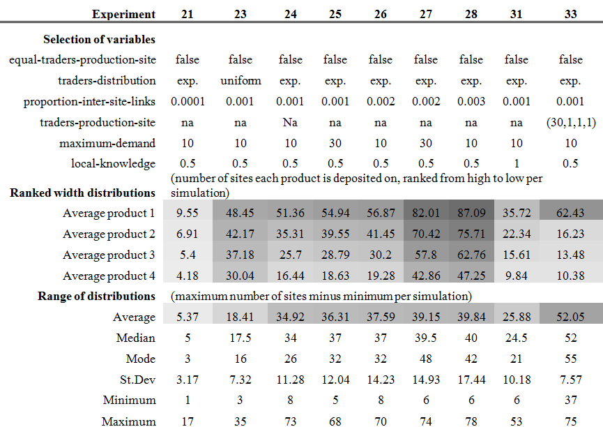
Comparison with randomly created networks
- 4.7
- Table 6 presents
results of experiments with the hypothesised social network structure
(experiments 22; 24; 25; 33) and experiments with the same independent
variable settings but with a randomly created network structure with
the same density (experiments 35; 29; 32; 34). The experiments with
randomly created networks give rise to more widely distributed products
in all tested cases. This is not surprising since the proportion of all
links that exist between pairs of traders on different sites is much
higher in experiments with randomly created networks than in those with
the hypothesised social network structure (Table 2).
However, the experiments with randomly created networks do not give
rise to high ranges of distribution (Table 6).
See in particular the average ranges of experiments 35 and 32, which
are much lower than those of experiments with the hypothesised social
network structure (experiments 22 and 25 respectively). However,
experiment 29 (randomly created network) shows a very similar average
range to that of experiment 24 (hypothesised network structure). As
illustrated in Figure 6, this
is caused by the very strong differences between iterations of the
experiment in the distribution of wares, and of the least distributed
ware in particular (ware 4 of experiment 29 in Fig. 6).
Finally, in experiment 33, strong differences in the number of traders
at each production site gave rise to one very widely distributed
product and three less widely distributed products. Note that this
reflects the archaeologically attested pattern described in section
Explaining pottery distributions that we aim to study here.
The
results of experiment 34 with a randomly created network and otherwise
the same variable settings as the latter experiment echo these results,
but show a higher range and wider average distribution for all four
products, as would be expected given the randomly created network
(Table 6; Fig. 7). This result suggests that the
hypothesised network structure is less important for giving rise to
widely distributed products and strong differences between
distributions in scenarios where one production centre produces a far
higher quantity of products than the other three.
Table 6: Selected variable settings and summary results for experiments designed to evaluate the effects of one independent variable: network-structure. The setting for traders-production-site for experiments 33 and 34 is given in brackets, because in each iteration of these experiments the number of traders at production sites A, B, C, and D was set to 30, 1, 1, and 1 respectively. See caption Table 3 for a detailed description of the information presented in this table. Note how the experiments with a randomly generated network structure have a higher width of distribution, but not necessarily a higher average range of distribution (with the exception of experiment 34). 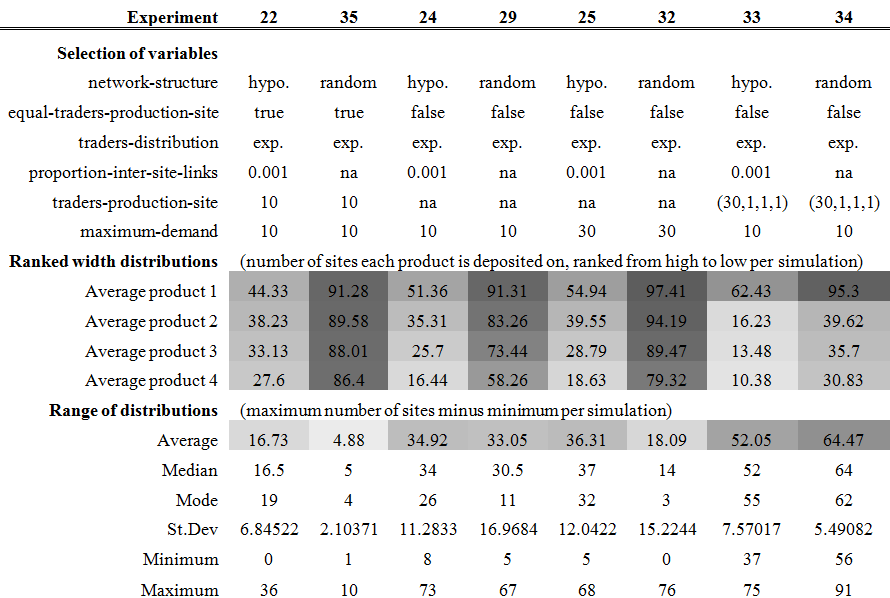
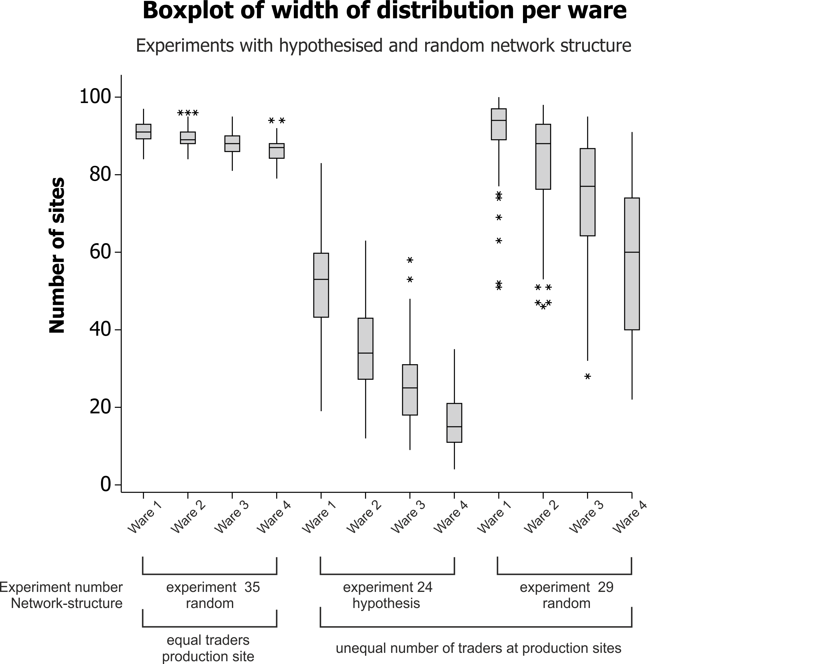
Figure 6. Boxplot of the width of distribution per ware for four experiments. Each boxplot combines the results of 100 iterations per experiment, and they represent the wares from the most widely distributed (ware 1) to the least widely distributed (ware 4). Note that the results of experiment 35 show widely distributed wares but with a very limited range of distributions between different types of wares. Experiments 24 and 29 have the same independent variable settings but for their hypothesised and randomly created network structures respectively. Their average ranges are similar but experiment 29 shows more widely distributed wares. See Table 6 for summary statistics and Supplement 1 for all independent variable settings for the experiments presented here. 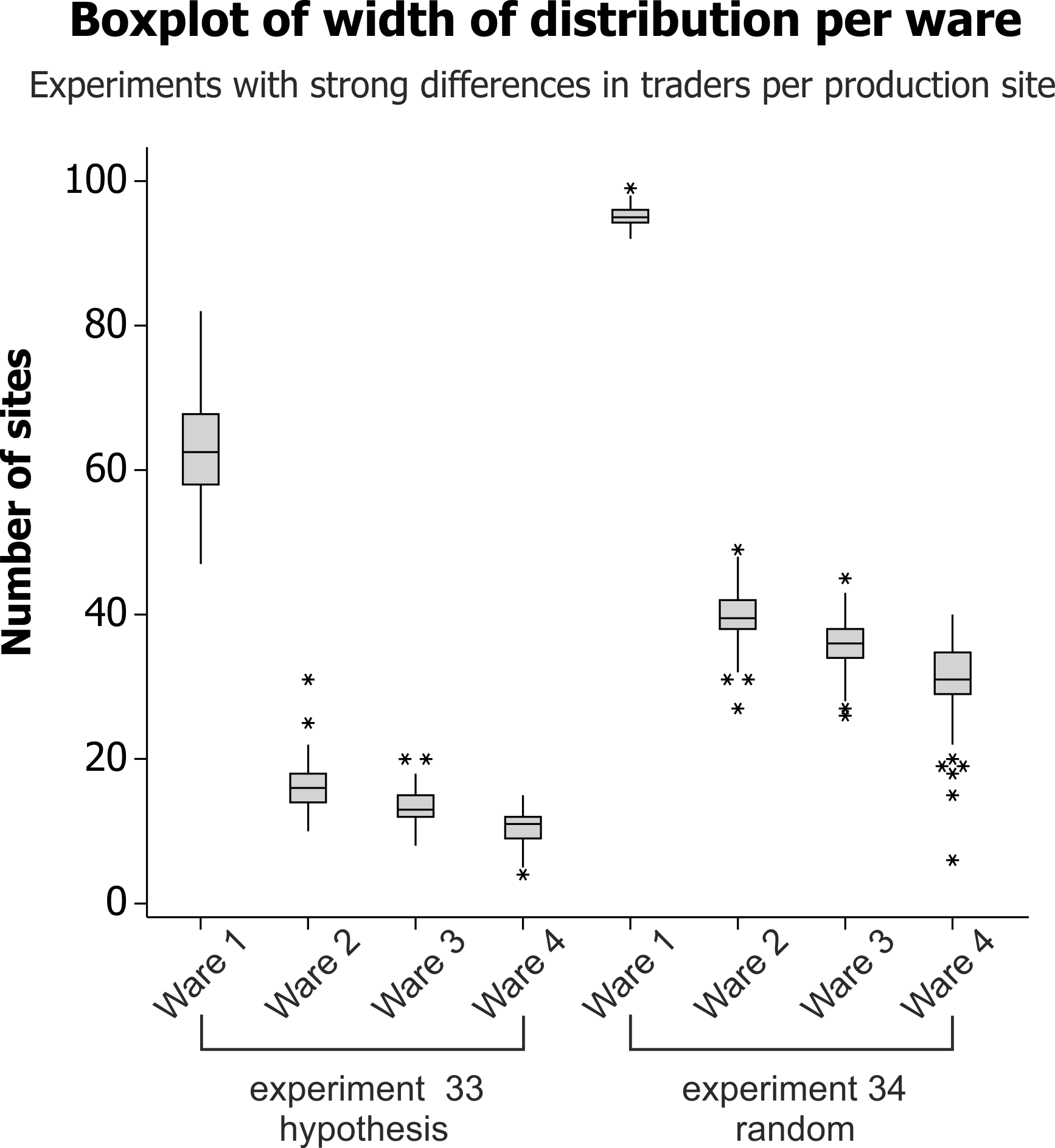
Figure 7. Boxplot of the width of distribution per ware for two experiments. Each boxplot combines the results of 100 iterations per experiment, and they represent the wares from the most widely distributed (ware 1) to the least widely distributed (ware 4). Experiments 33 and 34 have the same independent variable settings but for their hypothesised and randomly created network structures respectively. Note the similar range of distribution of both, and the similar pattern of one ware being far more widely distributed than the other three, but wares are more widely distributed on a randomly created network. See Table 6 for summary statistics and see Supplement 1 for all independent variable settings for the experiments presented here.
Discussion
and conclusions
- 5.1
- In this paper we have presented the conceptualisation and implementation of MERCURY, an Agent-based Model of Roman Trade, as well as the results of a series of experiments. This work represents the first attempts at formalising and simulating some of the hypotheses that aim to explain Roman tableware distributions using computational modelling (see Graham and Weingart (2015) for related work). To further clarify the potential of this approach, we will discuss the implications of the results, how they suggest some promising future research directions and ways of modifying and improving MERCURY to answer a wider range of research questions.
- 5.2
- The main results are represented in Figure 8 and indicate that the proportion-inter-site-links,
traders-production-site, and
max-demand variables positively correlate with the width of
distribution of all the products but not with the range of distribution
(i.e. not with strong differences in the distributions between products
similar to the ones observed in archaeological data). Secondly,
randomly created networks, which have a higher proportion of inter-site
links than the hypothesised social network structure, also give rise to
a wide distribution of all products but not to high ranges of
distribution (i.e. they show a small difference between the most widely
and least widely distributed products). The pattern of a strong
difference between the most widely and least widely distributed
products is achieved only in a scenario in which one production site
has far more traders and therefore has the potential of exporting more
produce than any of the others (see experiment 33). This result holds
true even when the hypothesised social network structure is replaced by
a randomly generated network (see experiment 34).
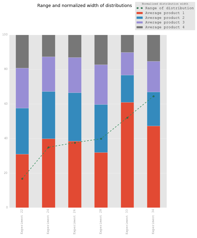
Figure 8. Range and normalized width of distribution for selected experiments. The pattern observed in the archaeological data (i.e. that one product is significantly more widely distributed and the difference in distribution width between this product and the least widely distributed product (range) is high, see Fig. 1) was only reproduced in scenarios where one production centre has far more traders than any other production centre and the number of inter-site links is high (proportion-inter-site-links 0.001) (see experiments 33 and 34). This pattern is not strongly affected by the proportion of available commercial information (local-knowledge). - 5.3
- The results presented here suggest that market integration in part might cause wide distributions of tablewares and differences in tableware distributions. However, market integration alone is not sufficient as an explanation. The potential of one production centre to produce far more than the others is a second necessary ingredient. Nevertheless, limited degrees of market integration are unlikely to result in wide tableware distributions and strong differences between the tableware distributions. We therefore argue that the emphasis on limited market integration in Bang's model is highly unlikely.
- 5.4
- The aim of this research was not to find an exact fit to the archaeologically observed data patterns, but to investigate elements of two conceptual models and produce predictions for each of them which can then be compared to broad archaeologically attested patterns. We have shown that some of the causal factors of the proposed conceptual models (e.g. changing the availability of commercial information from trade contacts) turn out to have less of an impact on generating the pattern of interest, while other factors show more promise in this regard (e.g. changing the degree of market integration). Under the conditions and assumptions imposed in this particular implementation of Bang's and Temin's conceptual models, our experiments suggest that future research into the functioning of tableware distribution processes should focus more on two factors: (1) actors and processes that enable market integration, and (2) the requirements to enable extremely high production of tableware consistently throughout long time periods. The former should include a closer look at the role of government and institutions in regulating trade and in providing incentives to individuals or groups of traders to supply for large demands, as well as into those commercial actors (individuals, communities, institutions) that had the financial and logistical means to gather reliable commercial information and trade between markets. The latter should include an examination of the possibility that historical contingency played a role in giving an edge to one type of tableware production centre over others, for example one tableware (ESA) being produced first and using the earlier development of distribution channels as an advantage to remain the dominant tableware in the Eastern Mediterranean. Moreover, it should be evaluated whether other factors hinted at in this model might have contributed to one tableware being more widely distributed, such as the existence of an urban hub close by the tableware production centre or region, which acts as a primary and stable source of demand for the product, and a productive hinterland able to supply the primary products and labour needed to supply for high demands.
- 5.5
- Moreover, the model could be improved by adding a market-clearing mechanism, a set or variable cost of transporting goods, and a more controlled conceptualisation of time. Finally, the model can be expanded to test some of the topics of future research interest suggested above by elaborating on the production processes, allowing for heterogenous traders with different rules of behaviour (which would leverage more the advantages of ABM than the current version of the model), allowing for changes in the social network structure, incorporating state influence, distinguishing between channels for the flow of information and those for the flow of goods, and considering transport costs. Some of these might require alternative conceptualisations to the one presented here.
- 5.6
- We have placed a particular emphasis here on illustrating that two conceptual models which stand for fundamentally different interpretations of the functioning of the Roman economy can be compared by abstracting them using the same set of concepts. Indeed, we argue that the conceptualisation is the most crucial stage of any computational modelling of the Roman economy and that it should be considered a task of the archaeologists and historians who create conceptual models. It should be clear that we do not argue that every scholar of the Roman economy should become a computer programmer. Instead, we believe that in order for the discussion on the functioning of the Roman economy to progress, scholars should (a) clearly define the concepts used and discuss exactly how these differ from the concepts used by others, (b) make explicit how these concepts can be represented as data, (c) describe the expected behaviour of the system using the defined concepts, (d) describe the expected data patterns resulting from this behaviour, and (d) define how (if at all) archaeological and historical sources can be used as reflections or proxies of these expected data patterns. By doing so, conceptual models of the Roman economy, as they are envisaged by their authors, hold the potential of being compared and falsified if the necessary archaeological or historical sources become available. These conclusions also do not imply the limitation of the study of the Roman economy to a single conceptual framework or a limited set of computational models. At this early stage of the use of computational modelling in Roman economy studies, multi-vocality of concepts and computational models is a virtue. What matters is to define how these differ and to develop them in ways that allow for comparisons between them.
- 5.7
- The study of the Roman economy is a fascinating and thriving discipline in need of methodological developments. We have shown here that agent-based modelling shows great potential in this respect, and argue that the use of computational modelling as a whole should become more common practice in the study of the Roman economy.
Acknowledgements
- This research was supported by the Belgian Programme on Interuniversity Poles of Attraction (IAP 07/09), the Research Fund of the University of Leuven (GOA 13/04), and Projects G.0562.11 and G. 0637.15 of the Research Foundation Flanders (FWO). Part of this paper was written during employment on the CARIB project, and financially supported by the HERA Joint Research Programme, which is co-funded by AHRC, AKA, BMBF via PT-DLR, DASTI, ETAG, FCT, FNR, FNRS, FWF, FWO, HAZU, IRC, LMT, MHEST, NWO, NCN, RANNÍS, RCN, VR and The European Community FP7 2007–2013, under the Socio-economic Sciences and Humanities programme. This work benefited from a research stay at the Belgian School in Rome, funded by a Stipendium Academia Belgica. We would like to thank Fraser Sturt, Andy Bevan, Simon Keay, Graeme Earl, Iza Romanowska, Viviana Amati, Arlind Nocaj and Mereke van Garderen for helpful comments on drafts of this paper.
Notes
- 1https://github.com/NetLogo/NetLogo/wiki/Extensions (accessed 05-01-2015).
References
- ABADIE-REYNAL, C. (1989).
Céramique et commerce dans le bassin Egéen du IVe au VIIe siecle. In V.
Kravari, J. Lefort, & C. Morrisson (Eds.), Hommes et
richesses dans l'empire byzantin. Tome I, IVe-VIIe siècle
(pp. 143–159). Paris.
BANG, P. F. (2008). The Roman bazaar, a comparative study of trade and markets in a tributary empire. Cambridge: Cambridge University Press.
BENTLEY, R., Lake, M., & Shennan, S. (2005). Specialisation and wealth inequality in a model of a clustered economic network. Journal of Archaeological Science, 32(9), 1346–1356. [doi://dx.doi.org/10.1016/j.jas.2005.03.008]
BES, P. (2015). The Distribution of Terra Sigillata and Red Slip Ware in the Roman East: a Chronological and Geographical Study. Oxford: Archaeopress.
BRUGHMANS, T., & Poblome, J. (2015). MERCURY: an ABM of tableware trade in the Roman East. CoMSES Computational Model Library. https://www.openabm.org/model/4347/version/2/view
BRUGHMANS, T., & Poblome, J. (2016). Roman bazaar or market economy? Explaining tableware distributions in the Roman East through computational modelling. Antiquity, 349/1.
GRAHAM, S., & Weingart, S. (2015). The Equifinality of Archaeological Networks: An Agent Based Exploratory Lab Approach. Journal of Archaeological Method and Theory, 22, 248–274.
GRIMM, V., Berger, U., Bastiansen, F., Eliassen, S., Ginot, V., Giske, J., … DeAngelis, D. L. (2006). A standard protocol for describing individual-based and agent-based models. Ecological Modelling, 198(1-2), 115–126. [doi://dx.doi.org/10.1016/j.ecolmodel.2006.04.023]
GRIMM, V., Berger, U., DeAngelis, D. L., Polhill, J. G., Giske, J., & Railsback, S. F. (2010). The ODD protocol: A review and first update. Ecological Modelling, 221(23), 2760–2768. [doi://dx.doi.org/10.1016/j.ecolmodel.2010.08.019]
JIN, E. M., Girvan, M., & Newman, M. E. (2001). Structure of growing social networks. Physical Review. E, Statistical, Nonlinear, and Soft Matter Physics, 64(4 Pt 2), 046132. Retrieved from http://www.ncbi.nlm.nih.gov/pubmed/11690115
LEWIT, T. (2011). Dynamics of fineware production and trade: the puzzle of supra-regional exporters. Journal of Roman Archaeology, 24, 313–332.
PEÑA, T. (2007). Roman pottery in the archaeological record. Cambridge: Cambridge University Press.
REYNOLDS, P. (1995). Trade in the Western Mediterranean, AD 400-700: the ceramic evidence. BAR international series 604 (Vol. 604). Oxford: Archaeopress.
TEMIN, P. (2013). The Roman Market Economy. Princeton: Princeton University Press.
WATTS, D. J., & Strogatz, S. H. (1998). Collective dynamics of "small-world" networks. Nature, 393(6684), 440–2. [doi://dx.doi.org/10.1038/30918]
WILLET, R. (2012). Red slipped complexity. The socio-cultural context of the concept and use of tableware in the Roman East (second century BC – seventh century AD). Unpublished PhD thesis. Katholieke Universiteit Leuven.