
 Abstract
- This paper presents an incremental method of parsimonious modelling using intensive and quantitative evaluation. It is applied to a research question in urban geography, namely how well a simple and generic model of a system of cities can reproduce the evolution of Soviet urbanisation. We compared the ability of two models with different levels of complexity to satisfy goals at two levels. The macro-goal is to simulate the evolution of the system’s hierarchical structure. The micro-goal is to simulate its micro-dynamics in a realistic way. The evaluation of the models is based on empirical data through a calibration that includes sensitivity analysis using genetic algorithms and distributed computing. We show that a simple model of spatial interactions cannot fully reproduce the observed evolution of Soviet urbanisation from 1959 to 1989. A better fit was achieved when the model’s structure was complexified with two mechanisms. Our evaluation goals were assessed through intensive sensitivity analysis. The complexified model allowed us to simulate the evolution of the Soviet urban hierarchy.
- Keywords:
- ABM, Model-Building, System of Cities, Former Soviet Union, Evaluation, Incremental
Introduction
- 1.1
- Systems of cities are complex social objects. They are identified by robust regular patterns of spatial and hierarchical organisation that are observed in various places and time periods worldwide. Such patterns derive from a common set of basic interurban processes, which are embedded in diverse geographical, economical and political contexts. This means that generic hypotheses about interurban interactions should hold in every contexts and contribute to explaining the observed urbanisation process, even in specific territories and periods such as the Soviet Union from 1959 to 1989. Can generative models help to distinguish generic and particular features of such systems of cities and their urban trajectories? Is there a generic core model of systems of cities that can simulate the evolution of the Soviet urban patterns? This paper presents the implications of the answer to these questions for the conception, building and evaluation of such models.
- 1.2
- The search for generic urban processes and mechanisms, translated into complex theories and models, started thirty years ago (Pumain & Sanders 2013). A recent shift occurred with the use of ABMs (Heppenstall et al. 2012). The flexibility and modularity of these models and their capacity to integrate agents' heterogeneity are helpful in comparing different model structures, different levels of model complexity and the effect of different contexts. They are now commonly used as virtual laboratories for hypotheses testing (Batty & Torrens 2001). However, there is no common standard technique to evaluate ABMs. Consequently, many modellers tend to postpone evaluation until the end of the modelling process, if not indefinitely (Amblard et al 2007). "A brief survey of papers published in the Journal of Artificial Societies and Social Simulation and in Ecological Modelling in the years 2009–2010 showed that the percentages of simulation studies including parameter fitting were 14 and 37%, respectively, while only 12 and 24% of the published studies included some type of systematic sensitivity analysis" (Thiele et al. 2014, §1.4). Feedback from evaluation is also seldom used in an explicit way to improve the features of models.
- 1.3
- We think that explicit feedback from model evaluation offers two opportunities: first, it strengthens the conclusions drawn from the model (e.g. on the validity of the involved mechanisms and the reliability of predictions drawn from various scenarios). Second, revealing unsuccessful mechanisms and unrealistic model behaviours helps in understanding the system under study and in improving theory. We propose in this paper a path toward complexification of an ABM using quantitative and replicable evaluation of each successive increment of the model. We started with the most parsimonious version including the most basic hypotheses on urban interactions. We then added supplementary mechanisms, only if necessary, following a stepwise progression. This conventional method of modelling (Epstein & Axtell 1996; Grimm & Railsback 2012) is here backed up by a large-scale toolbox for automatic and quantitative evaluation.
- 1.4
- At each step of the progression, the outputs of the model were compared to empirical data. This enabled calibration of the model according to explicit and quantified goals. Calibration and sensitivity analysis quantified the ability (or failure) of the current version of the model to fit defined goals, by extensively exploring its parameter space. These explorations allowed us to detect micro- and macro-behaviours exhibited by the model and its mechanisms. In case of failure to meet calibration requirements, these properties helped us to understand how the model could be complexified to improve its performance and dynamics. By doing so, we claim to get closer to social science theory and practice, which usual abductive method (for choosing the content of the model, the type of agents, main attributes and rules of change) is included in a method integrating a quantitative and automatised evaluation at each step of an incremental model-building process.
- 1.5
- This evaluation-based incremental modelling method (EBIMM) is implemented in this paper through building the first models of the MARIUS[1] family. MARIUS is a family of models which aims at reproducing demographic trajectories of cities in the post-Soviet space. The theoretical background of systems of cities' modelling, experiences and stakes will be presented in Section 2, which will also describe the MARIUS contribution to this field and the way we propose to disentangle generic from specific mechanisms within an incremental framework for model-building (supported by systematic evaluation of resulting increments and models). Section 3 provides a detailed description of the mechanisms included in the most parsimonious model (yet complex enough to capture the basic features of systems of cities). Section 4 summarises the evaluation of this first model and the detection of unwanted model behaviours. They disqualify this parsimonious model as offering an insufficient set of mechanisms to meet our evaluation requirements. Section 5 shows that adding only two more mechanisms, and thus minimising complexification, is sufficient to reproduce realistic dynamics of the system of Soviet cities and its structural evolution. The paper ends with a discussion of the advantages of using this method to produce reliable geographical insights (Section 6).
Modelling systems of cities
-
Theory and existing models
- 2.1
- The urban theory on which we base our research (Pumain 1997) proposes an evolutionary and complex account of the regularities observed in a large number of systems of cities over time. The well-known organisation of cities in space and the regular distribution of their size has given way to many possible explanations, mostly static (optimisation of consumption patterns (Christaller 1933)), least effort principle (Zipf 1949) and/or stochastic (Gibrat 1931; Simon 1955). However, stochastic models have proven unable to cope with systematic deviations from Zipf's rank-size rule observed empirically. By acknowledging that the evolution of urban systems includes elements of "chance and determinism" (Allen & Sanglier 1981, p.168), new theories have included synergetic and complexity principles to explain the emergence[2] of a hierarchical structure in systems of cities (Pumain 2006; Batty 2007). They assume that systems of cities are emerging from the repeated and diversified interactions between cities. Systems of cities are characterized by macro-scale properties, such as hierarchy (the uneven distribution of city sizes), a regular spatial structure and functional diversity. The macro-scale corresponds to that of nation-states or continents, i.e. a time-distance of roughly one day to connect any pair of cities. The functional integration of cities, through repeated and sustained patterns of interactions, is indeed thought to operate preferentially at this scale (Pumain 2006). Temporally, because of the succession of innovation cycles favouring large cities on average for being first adopters, the theory assumes that hierarchy and hierarchisation (i.e. the accentuation of the degree of hierarchy) tend to emerge together with the specialisation of cities according to their size and functions. Large cities benefit from a diversified range of activities and are early adopters of innovations, which benefits them in terms of growth and development in their next period of development. Whereas, small cities tend to specialize more deeply, accelerating their development rate as well as their decline when the innovation cycle changes. Finally, the distribution of growth follows a non-random spatial pattern, derived from political divisions on the one hand, and on the other, a process of spatial concentration of population, wealth and innovation creation.
- 2.2
- The study of these emerging properties relies on the
observation of systems of cities through harmonised spatio-temporal
databases. Their systematic comparison leads the identification of
empirical
regularities and fosters theory building (Bretagnolle
et al. 2009; Pumain et
al. 2015). Different modelling strategies have been pursued
to study systems of cities: statistics, differential equations,
synergetic, etc. The agent-based paradigm seems a promising one for
geographers (Bretagnolle et al.
2006; Heppenstall et
al. 2012; Pumain
& Sanders 2013), because of its ability to capture
the richness and diversity of cities (Batty
et al. 2012). First attempts at simulating the emergence of
hierarchy in a settlement system were conducted with the Simpop model,
the first to consider cities as agents (Bura
et al. 1996; Sanders et
al. 1997). With the introduction of competition between
cities, stochasticity and the adoption of urban functions, the
implementation of theoretical propositions proved successful at
generating the main patterns of systems of cities. Simpop2 and Eurosim
models (Sanders 2007; Bretagnolle & Pumain 2010)
went further by taking into account a larger number of cities,
functions and interaction types, as well as empirical data for
evaluation. However, these models proved very complex and difficult (if
not impossible) to calibrate. Evaluation, thought of late in the
process of model-building, made it difficult to draw conclusions from
the
results of the model, and left unresolved important questions such as
that of
the influence of data-injection in the simulated dynamics. Further
research conducted within the Simpop project aimed, with SimpopLocal,
at building more parsimonious models better suited for evaluation and
sensitivity analysis. It led to the development of automated and
distributed methods for evaluating the ability of a parsimonious
model to reproduce stylised patterns (Schmitt
et al. 2015; Reuillon
et al. 2015).
A new incremental framework
- 2.3
- The MARIUS project benefits from this double inheritance. First, it represents a new case study for the urban theory to be tested on: Soviet cities. We aimed at determining to what extent this system of cities can be considered generic and/or specific. Answering this question with standard statistical models and a harmonised database was the first step towards answering this question, but it showed that this system exhibits generic features (hierarchical distribution for example) as well as particularities (shape and level of hierarchy for example) (Cottineau 2013; Cottineau 2014). It gave rise to the formulation of several hypotheses to be implemented incrementally as mechanisms.
- 2.4
- We built a framework for incremental generative modelling by hierarchizing possible mechanisms accounting for the post-Soviet urban evolution, from the most generic ones to the supposedly most specific to the Soviet Union. These mechanisms are based on data and covariations revealed by statistical analyses. They go beyond covariation by asserting a causal relationship between cities' attributes and demographic trajectories. We specified two axes of complexification of the model mechanisms (Fig. 1): axis 1 exposes mechanisms of increasing complexity (from left to right) in terms of interactions between agents, axis 2 exposes mechanisms of increasing complexity (from bottom to top) in terms of the geographical environment with which agents (cities) interact.
- 2.5
- For instance, along the first axis, we consider spatial interactions as being the common set of mechanisms that govern cities' structuration and co-evolution (i.e. the most generic feature characterizing systems of cities in the world). Adding territorial redistribution via taxes collected within political boundaries gives a more complex model in terms of agents' interactions. Redistribution is common to different systems of cities, yet more specific to the understanding of Soviet urbanisation (Iyer 2003). We also plan to add mechanisms locking and differentiating interurban economic exchange networks, as we know that the functional specialisation of cities was particularly important in the Soviet Union (Harris 1970, p. 484; Snyder 1993; Lappo & Polyan 1999), with the presence of monopoly firms and mono-industry towns. Finally, the most specific mechanism would allow a meta-agent to be in charge of investments and new towns creation, reflecting the way in which central planning in the USSR operated.
- 2.6
- Along the second axis, firstly, we consider the importance of resource extraction in the economic and demographic trajectories of cities. Secondly, the importance of a rural reserve of migration in the differentiation of urbanisation in the regions. Thirdly, the particular role of transportation infrastructures in such a gigantic space. The most specific set of mechanisms include boundaries opening or closing with an outside world depending on the geopolitical context.
- 2.7
- For each mechanism at a given complexity level, we may
propose several alternative implementations (axis 3).
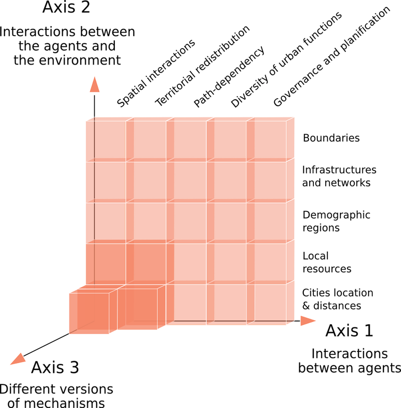
Figure 1. A map of incremental implementation of generative mechanisms within a family of models - 2.8
- We think that all these mechanisms potentially contribute to explaining the evolution of cities during the end of the Soviet Union, but instead of adding all the mechanisms at once, we want to get an insight into the "share of explanation" possessed by the most generic mechanisms. The cornerstone of this family of models, on which this paper focuses, is the first, low-level "block" of the map. It includes only generic mechanisms that can be applied to other systems of cities. The agent-based framework is therefore not entirely necessary to implement this first model, in which agents have no heterogeneous, moving or stochastic behaviour. However, those properties will be implemented as we increase complexification, which is why we implement this first model as an agent-based model.
- 2.9
- Model evaluation is acknowledged from the start in the model-building process: we use calibration and sensitivity analysis throughout the implementation of the models and compare simulations with empirical data collected about cities in the post-Soviet space[3]. By doing so, at each step of complexification of the model, we can estimate the extent of its contribution to the explanation of observed dynamics. In addition to expliciting the modelling process, EBIMM fits our research question, which is: to what extent do we need to particularize a model of system of cities' dynamics in order to reproduce the actual evolution of cities in the post-Soviet space? We illustrate the advantages of this approach in the following sections with the cornerstone MARIUS model. This cornerstone model relies on very generic mechanisms drawn from urban theory. In its most abstract form, it is composed of spatial interactions and agglomeration economies.
A skeletal model of urban evolution
- 3.1
- We describe the first MARIUS model using parts of the ODD
protocol (Grimm et al. 2006)
to organize its outline. For a full description of the model with ODD,
as well as implementation details and codes for model execution,
fitness computation and visualization, please refer to the
documentation online[4].
ODD. Purpose
- 3.2
- This model targets a particular system in a specific
time-span: the Soviet system of cities, from 1959 to 1989. It seeks
to identify a minimal set of interaction mechanisms able to simulate
stylised facts (or patterns) observed in the actual system. Once again,
we acknowledge the singularity of the spatio-temporal urban perimeter,
but instead of stating it ex ante, we use generic
mechanisms and models to assess its degree of particularity by
reference to the evolution of what would be a "standard" system
embedded in the Soviet environment in 1959 up to 1989. This time-span
is one of relative stability in the Soviet Union, thus allowing for
"basic" urban mechanisms to play the main role in the evolution of
cities[5].
We evaluate these urban mechanisms by comparing their output to
empirical patterns drawn from successive census data. Patterns refer to
structural characteristics commonly used by geographers to qualify
systems of cities: their hierarchization, the spacing of cities across
the territory, and their functional differentiation (see 2). Interaction mechanisms
are intended to model repeated exchanges (goods, services, information
and
persons) between cities over time.
ODD. Entities, State variables, Scale
- 3.3
- The system is made of 1145 urban agglomerations (we use the
shorter term city henceforward) of more than 10,000
inhabitants in 1959, localised at their actual latitudes and longitudes
(Fig. 2). They are the only
type of agent, and are characterised by a unique low-level variable to
be
compared with empirical data: their population. From
this single variable are derived economic variables involved in the
interactions mechanisms described below.
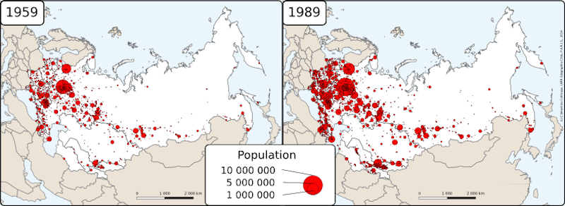
Figure 2. Empirical spatial and hierarchical distribution of cities in the post-Soviet space
source: DARIUS, 2014ODD. Processes overview and scheduling
- 3.4
- Time is modelled in discrete one-year steps[6] during which
interactions occur in a synchronous way. At each step:
- cities update their supply and demand.
- each city interacts with the others according to the intensity of their interaction potential. For two distinct cities, A and B, an interaction consists in relating A's supply to B's demand, resulting in a transaction of value from A to B.
- cities update their wealth depending on the transactions in which they were involved.
- cities update their population according to their new wealth.
ODD. Details
Initialisation: Cities-agents described by levels of population and wealth
- 3.5
- At initialisation, cities are characterized by their actual
geographical location and population, and by an estimated wealth. There
is empirical evidence for locations and populations. However, the
wealth of cities is a dimension that exists, but it is
not measured in the Soviet census data. We know from other national
studies that urban wealth covaries with population: scaling
regressions of wealth (or income) against total population have been
found to be super-linear, with an exponent of 1.12 in the USA, 1.15 for
China, 1.26 in Europe (Bettencourt
et al. 2008, p.287). This means that large cities are
proportionally richer than small ones, due to concentration processes
(among which are urbanisation and agglomeration externalities, (Marshall 1920; Fujita & Thisse 1996).
Therefore, we estimate the wealth of cities at initialisation by means
of a superlinear scaling relation with population (Eq.1)[7].
$$wealth_i = population_i^{populationToWealthExponent}$$ (1) - 3.6
- We choose not to model the mechanisms relating to prices
and currency. We therefore consider wealth as a concept of absolute
value centered on the mean of the population distribution at
initialisation. The quantity is irrelevant to our model as we rather
focus on the uneven distribution of wealth among cities. The exponent
of the initial scaling law is set to range over 1. It has been
empirically
observed to vary between [1.1;1.3]. We extend this
interval to [1;10] in the calibration of the initial wealth stock
(known as
being usually 4 to 8 times greater than the flow of wealth per year at
the scale of countries (Piketty 2013).
Box 1 The fact that the Soviet Union was a planned economy does not mean that money or economic processes did not exist, nor that the Soviet city in "incomparable" with its western equivalent (French & Hamilton 1979). It is supposed to mean that production capacities, interactions and prices were planned "from above" (Manove 1971), and that the distribution of productive forces was a potential tool for its realisation (Khorev 1975). However, numerous levels of adaptation and bargain distorted this idealised vision in the everyday Soviet economy (Neuberger 1968). This resulted in a dual system of prices, one official price and the actual value given to labour as well as goods, with the adjustment between them taking the form of migration, services and informal arragements. This validates our decision to model an abstract value for production and exchange unit. Finally, the hypothesis of agglomeration economies, a concept developped in liberal economies, seems to apply to the Soviet Union as well. Striking support to this idea is offered by the constant search of Soviet planners for an "optimal city size" (Khorev 1975; Iyer 2003) and their constant failure to restrict big cities' size (Gang & Stuart 1999). Updating economic variables
- 3.7
- At the beginning of each step, we compute the annual
production and consumption values for each city. They vary as a
function of:
- the city population,
- a parameter adjusting this value to the fictional unit of wealth,
- a scaling exponent stressing the effect of size on productivity and consumption per capita.
- 3.8
- From the supply side, the advantages of large cities are
acknowledged as agglomeration (Fujita
& Thisse 1996; Puga
2010) and urbanisation (Henderson
1986) economies.
Productivity per capita is higher in large cities because of a larger
capital stock being available and shareable for each unit of labour,
because
of better skill matching and fluidity between labour supply and demand,
and
because of the concentration of human capital, the opportunity of
learning
and the possibility of an inner division of labour within the city (Duranton & Puga 2004).
Likewise, income per capita and living standards are higher in larger
cities. "Controlling for differences in culture and economic
development, incomes per capita tend to rise with city size."
(Batty 2011, p.385). In the
Soviet "classless society", where policies promoted income and spatial
equality, there is still evidence of informal and non-monetary
compensation to elites and privileged groups. These were concentrated
in the largest urban centres (French
& Hamilton 1979). Supply and demand are therefore
defined here as they would be in any other system of cities, by:
$$ \begin{array}{ll} & Supply_i = EconomicMultiplier \ast population_i^{sizeEffectOnSupply}\\ \mathrm{with} & EconomicMultiplier > 0\\ \mathrm{with} & sizeEffectOnSupply \geq 1\\ \end{array} $$ (2) $$ \begin{array}{ll} & Demand_i = EconomicMultiplier \ast population_i^{sizeEffectOnDemand}\\ \mathrm{with} & EconomicMultiplier > 0\\ \mathrm{with} & sizeEffectOnDemand \geq 1\\ \end{array} $$ (3) - 3.9
- The exponents sizeEffectOnSupply and sizeEffectOnDemand
in equations 2 and 3 represent the magnitude of agglomeration effects
on urban supply and demand levels. The larger they are, the more cities
are unevenly productive and consumptive relative to their size.
Similar exponents have been used recently to compare the scaling
behaviours
of different systems of cities (Bettencourt
et al. 2008). The sizeEffects on the supply
and demand parameters' bounds for calibration are
derived from these scaling estimations using income per capita
("consumption") or added value per capita ("productivity") (observed
empirically in the range [1.1;1.3]). Supply and Demand size effects can
differ but they share the same range of possible values for the
calibration ([1; 10]). For the economicMultiplier
parameter, we have no empirical insight about the value it should take
since it serves as a factor adjusting the fictive wealth value. Its
calibration range is therefore set very large ([0; 1000]), and its
absolute value is not interpreted per se.
Spatial Interaction model
- 3.10
- Based on their supply, demand and distance, we computed a
value of potential interaction for each pair of cities, using a gravity
model. This model has been used in geography since E. G. Ravenstein (1885). It estimates
accurately the expected flows between places, because it captures some
obvious properties of spatial interactions: large places are more prone
to exchange with other places than smaller ones and close places tend
to exchange more with one another than distant places. The description
of this relation is given by Eq.4:
$$ F_{ij} = k \ast \frac{M_i \ast M_j}{d^{distanceDecay}} $$ (4) with k being a normalisation constant, \(M_i\) and \(M_j\) characterizing masses of cities i and j (population, wealth, jobs, etc.) and \(d\) the distance between them (in km, hours, cost, etc.)
- 3.11
- Following T. Hägerstrand and numerous geographers after him
(see Sanders 2001), we
can consider \(F_{ij}\) as a proxy for the interaction potential (or
field
of opportunity) between cities \(i\) and \(j\). In our representation
of the exchange market, the masses \(M\) are the supply of city \(i\)
and the demand of city \(j\), resulting in an asymetric matrix of
potential interactions. We use the geodetic distance separating two
cities in the denominator. The distanceDecay
parameter represents the magnitude of variation of the potential
interaction as distance between two cities grows. The higher this
parameter, the less likely distant interactions are to happen (or the
smaller they get). Estimation of the distanceDecay
parameter has
been computed for a large number of empirical cases studies. The
maximum bounds identified in the literature reviewed by Fotheringham (1981) in interregional
examples vary from \(-0.3\) (the distance between two places stimulates
the potential of interaction) to 5.2 (the constraint of distance over
interaction is very strong). In an interurban context, Baccaïni
& Pumain (1998)
find lower values for this parameter: between 0.5 and 1 depending on
the measured flows. We restrict the minimum value of distanceDecay
to 0 (the distance plays a decreasing or no role in the interaction
potential), and the maximum to 10. Finally, \(k\) adjusts interaction
potentials to the measurement unit. Since we focus on ratios of
interaction potentials, we exclude this parameter from the MARIUS
model, and use equation 5:
$$ InteractionPotential_{ij} = \frac{Supply_i \ast Demand_j}{d^{distanceDecay}} $$ (5) A city \(i\) allocates a share of its supply \(S_{ij}\) to a city \(j\). This share is proportional to the share of the interaction potential \(F_{ij}\) that city \(j\) represents in the total interaction potential of city \(i\) as a producer:
$$ S_{ij} = Supply_i \ast \frac{F_{ij}}{\sum_k F_{ik}} $$ (6) Symetrically, a city \(i\) allocates a share of its demand \(D_{ij}\) to a city \(j\). This share is proportional to the share of the interaction potential \(F_{ji}\) that city \(j\) represents in the total interaction potential of city \(i\) as a consumer:
$$ D_{ij} = Demand_i \ast \frac{F_{ji}}{\sum_k F_{ki}} $$ (7) The effective transaction from city \(i\) to city \(j\) is determined as the minimum allocated value between \(i\) and \(j\):
$$ Transacted_{ij} = \min (S_{ij}, D_{ji}) $$ (8) When all transactions have been computed, we sum the gains and losses of the city to update its wealth:
$$ \begin{array}{ll} & wealth_{t,i} = wealth_{t-1,i} + S_i- D_i- unsold_i + unsatisfied_i\\ \mathrm{with} & unsold_i = Supply_i- \sum_j Transacted_{ij}\\ \mathrm{with} & unsatisfied_i = Demand_i- \sum_j Transacted_{ji}\\ \end{array} $$ (9) Interactions in the model consist of exchanges of value between cities. It is used as a proxy for many diverse transactions involving information, capital, goods and services. Human migrations are not part of this interaction mechanism. Instead, it modelled as a consequence of interactions: cities getting wealthier attract more people than cities in economic decline.
Translating wealth variations into population variations
- 3.12
- This conversion function between wealth and population is
based on the hypothesis that a gain of the same amount of wealth is
converted into a gain of a population that varies according to city size[8]. However, we do not
know with certainty from the literature if this relation is super- or
sub-linear. Orientation of causality (if it exists) between city size
and productivity and the ratio of agglomeration economies over negative
externalities (pollution, congestion, etc.) are not known (Ciccone & Hall 1996; Combes & Lafourcade 2012).
Should the conversion of gains in
wealth be a decreasing (\(wealthToPopulationExponent < 1\)) or
an increasing (\(wealthToPopulationExponent < 1\)) function of
elasticity with the city size? We let the calibration find the best
qualitative answer to this question. Therefore, the last parameter
(\(wealthToPopulationExponen\)) is left free to vary around 1 (Eq. 10).
$$ \frac{\Delta population_i}{\Delta t} = \frac{wealth_{t,i}^{populationToWealthExponent}- wealth_{t-1,i}^{populationToWealthExponent}}{EconomicMultiplier} $$ (10) We end each step of the model by computing the new population of cities as follows:
$$ population_{t,i} = population_{t-1,i} + \frac{\Delta population_i}{\Delta t} $$ (11)
Evaluation of the model
-
A first model parsimonious but unrealistic
- 4.1
- In order to assess the extent to which the model is able to
reproduce the hierarchical patterns of the actual system of Soviet
cities, we use an automatic calibration process of the six free
parameters, based on an evolutionary algorithm. To achieve this
numerical analysis, a quantified estimation of the distance of the
model to the expectations is defined. This distance is given by the
difference between the sorted distribution of simulated populations and
the empirical distribution. We compute the quadratic error between
simulated (log) populations and empirical (log) populations from data:
$$ DistanceToData(t) = \sum_i (\log(population_{t,i})- \log(dataPopulation_{t,i}))^2 $$ (12) with \(population_{i,t}\) the simulated population of the \(i\)th city at time \(t\) and \(dataPopulation_{i,t}\) being the empirical population of the \(i\)th city at time \(t\) in the data[9]. In the considered time span, we refer to data at four consecutive censuses. Censuses are performed every ten years or so, giving cities populations for dates \(t\) in \(\{1959, 1970, 1979, 1989\}\). The model is initialised with the empirical population in 1959 (\(dataPopulation_{1959,i}\)) and simulation results are evaluated by taking the sum of \(DistanceToData\) values for each available census date afterwards, i.e.:
$$ CumulativeDistanceToData = \sum_{t\in \{1970,1979,1989\}} DistanceToData(t) $$ (13) - 4.2
- The minimisation of this cumulative distance (or error) will be the first (and for now unique) goal of the calibration process. In order to calibrate the model we have used the NSGA2 genetic algorithm. This algorithm has been distributed on the European computing grid EGI using an island parallelisation strategy, in the same manner as in Schmitt et al. (2015). To make this large scale numerical experiment reproducible, we have implemented it on top of the free and open-source OpenMOLE plateform[10] for large scale experiments on simulation models. The complete calibration workflows, including the parameters of the calibration algorithm and of the distributed execution, have been made available online[11]. OpenMOLE relies exclusively on free software and all the implementation details of the genetic algorithm (GA) we have used can be found in the MGO library[12].
- 4.3
- The calibrated first model is quite close to empirical
data: \(distanceToData = 2.6541633574412\). This quadratic error
roughly corresponds to a difference of 12 million inhabitants for each
census, out of about 100 million total population. We find a trend
towards growth and hierarchization of the simulated system comparable
to that of the target system. Moreover, the distributions of city sizes
are quite similar at the three successive dates of observations,
especially for cities below the first ten ranks (Fig. 3). We also find values for half of
the parameters that are close to the empirical ranges (Tab. 2).
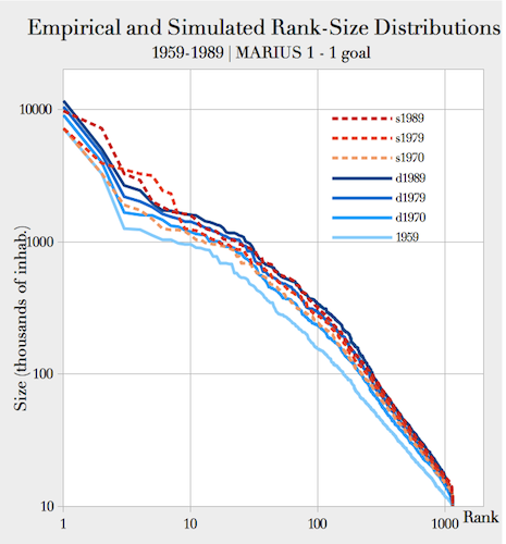
Figure 3. Comparison of empirical and simulated rank-size distribution of cities
Note: "d" stands for data and "s" for simulationTable 1: Best calibration of free parameters of the first MARIUS model Free Parameters empirical interval Reference for empirical intervals calibrated value \(populationToWealthExponent\) > 1 Bettencourt et al. 2008; Piketty 2013 1.00000068303 \(sizeEffectOnSupply\) \([ 1; 1.3 ]\) Bettencourt et al. 2008; Combes & Lafourcade 2012; Xu 2009 4.36280319382 \(sizeEffectOnDemand\) 7.84110925210 \(EconomicMultiplier\) - 99.99998687556 \(distanceDecay\) \([ -0.3; 5.2 ]\) Fotheringham 1981; Baccaïni & Pumain 1998 5.233129875642 \(wealthToPopulation Exponent\) - 0.310532195772 - 4.4
- However, the best performing models are those with
surprisingly high values for \(sizeEffectOnSupply\) and
\(sizeEffectOnDemand\) parameters, leading to unrealistically high
supplies and demands of cities, causing an "overflow" in the
interactions. A statistical summary of supplies and demands quantities
obtained with the parameters values of the best candidate reveals this
problem (Fig. 4). The best
model enables cities to exhibit disproportionate demand values (flows)
compared to stock variables. This "overflow" feature is not consistent
with economic findings (for example, Piketty's (2013)) which state that the
value of accumulated wealth is several times that of income produced
(\(Supply\)) or distributed (\(Demand\)) for the year of observation.
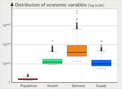
Figure 4. Economic variables of cities at the last step of a simulation with the best calibration of parameters of the MARIUS 1 model - 4.5
- Moreover, we observe a bias in the way the model is
optimized to reduce distance to data. In fact, a significant share of
cities (149 on average among the 1145 simulated cities at each step)
are deprived from their entire wealth in the course of the simulation.
This happens mainly to large cities (for example: Saint-Petersburg
loses all its wealth during the first step of simulation), cities
located near other large cities (typically, in the Moscow region) or in
densely settled areas (coal mining basins like the Donbas). We suppose
that this pattern results from the disproportionate values of demand
for cities with high interaction potentials. They are able to satisfy a
large amount of their demand (deduced from their wealth, cf. eq. 10)
without being able to "sell" much of their supply. Because we do not
allow negative wealth in the model, those cities are therefore bound to
stagnate until the end of the simulation. This sequence is neither
satisfactory nor realistic.
A first model: parsimonious but insufficient
- 4.6
- If the macro-level dynamics are satisfying (low distance to
data over time), the micro-level dynamics do not match our
expectations:
some cities lose all their wealth, and cease to be part of the
interaction. In order to prevent overflow, we introduce the following
quantity into
the evaluation function of the model:
$$ OverflowRatio(flow_i) = \left\{ \begin{array}{ll} \frac{flow_i}{wealth_i} & if~flow_i < wealth_i\\ 0 & otherwise\\ \end{array} \right. $$ (14) with \(flow_i\) being either \(supply_i\) or \(demand_i\). This measure is then summed for all time steps. For each city, it gives a \(TotalOverFlowRatio\):
$$ TotalOverflowRatio_i = OverflowRatio(Supply_i) + OverflowRatio(Demand_i) $$ (15) - 4.7
- The expected behaviours of cities consist in having supply
and
demand flows lower than their wealth stock, i.e., a
\(TotalOverFlowRatio\) of zero. This new (quantified) requirement is
integrated into the calibration process. From now on, calibration has
the goal of minimising three quantities:
- the \(CumulativeDistanceToData\)
- the number of cities whose wealth fell below zero during simulation
- \(TotalOverflowRatios\) of cities
- 4.8
- The calibration purpose is to identify parameters which realize the best compromise between these objectives. In comparison to the previous evaluation, the model's complexity remains the same, but the selection of candidates models is tighter. "Good" models are still those which produce results close to data over time, but without withdrawing any city from the interactions, or producing unrealistic flows of supply and demand[13].
- 4.9
- We consider this new requirement to be an improvement, as
it
allows to identify the more interesting models with realistic
micro-dynamics.
However, in the best calibrated models, interactions are much reduced
(by a very high \(distanceDecay\) and a very small
\(economicMultiplier\)) and the macro results are less satisfactory
(\(distanceToData = 12.5319231911183\); about 22 million people
differing
from the empirical distribution per census). Typically, cities exhibit
very small values for supply and demand, and the trajectories are very
chaotic (for the total urban population and the largest cities). At
this point, we show that this most parsimonious model cannot satisfy
both calibration objectives (no overflow and closeness to data). We
verify this trade-off with the pareto front of the 62 best sets of
parameters having finite values of overflow after more than 100.000
generations of the genetic algorithm (Fig.5).
This Figure shows that the algorithm has not found any combination of
parameters that would improve one of the calibration objectives without
degrading the other[14].
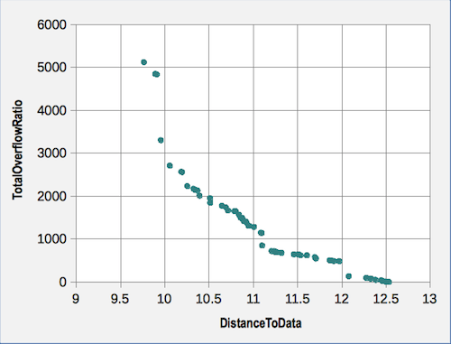
Figure 5. Pareto front between two objectives of calibration in the core model - 4.10
- In this section, two formalisation processes have been undertaken. The first is a standard one in socio-spatial simulation: it consists in the implementation of theoretical hypotheses as mechanisms. In the case of systems of cities within an evolutionary theory, it means giving the leading role to interurban interactions. The second one is less commonly undertaken and consists in formalising our expectations about what we mean by "good dynamics" in the form of (possibly antagonistic) computable objectives. These objectives guide the exploration of the model parameter space during calibration. By doing so, external knowledge is iteratively added to the evaluation of the model, resulting in a much more precise selection of realistic model candidates. This analysis has shown that it is not possible, at the lowest level of structural complexity of the model, to achieve simultaneously plausible dynamics and closeness to observed data. We need to refine the model to overcome this limitation.
A good cornerstone model candidate
- 5.1
- Qualitatively, the results above show an undesired trend towards abrupt growth and decrease in city sizes, especially at the top of the urban hierarchy. Creation of wealth and exchanges are very limited and merely redistributed within the system.
- 5.2
- In this section, we describe a new mechanism intended to
optimise the effective wealth creation without challenging the whole
model structure. This refined model will be termed Model 2.
Unlike Model 1, in which interurban exchanges are a zero-sum game
(there is no advantage for a city to exchange with the others rather
than producing and consuming internally, cf. eq. 9), Model 2 features a
non-zero sum game through a mechanism of bonuses, rewarding city-agents
who
effectively interact with others rather than internally. We assume that
the exchange of any unit of value is more profitable when it is done
with another city, because of the potential spillovers of technology
and information (Henderson 1986;
Glaeser et al. 1992; Castells 1996). This "bonus"
term will depend both on the total volume that a city has exchanged
with other cities and on the diversity of its external partners. It is
made
comparable to the fictive unit of wealth by the parameter
\(bonusMultiplier\):
$$ Bonus_i = bonusMultiplier \ast \frac{(importVolume_i + exportVolume_i) \ast partners_i}{n} $$ (16) with:
\(importVolume_i\) the total value bought from other cities
\(exportVolume_i\) the total value sold to other cities
\(partners_i\) the number of cities with which i has exchanged something
\(n\) the total number of cities (\(n = 1145\)) - 5.3
- Such a bonus given to cities needs a counterpart. It is
modelled by a mechanism of costs associated with interurban exchanges.
This cost is not proportional to distance (already taken into account
by the interaction potential). Exchanges are indeed costly in terms of
transportation, but economists also include transaction costs (Coase 1937) associated with the
preparation and realisation of the exchange (Spulber
2007). Our modelling choice for this cost mechanism is to
consider that every interurban exchange generates a fixed cost (the
value of which is described by the free parameter \(fixedCost\)). This
implies two features that make the model more realistic: first, no
exchange will take place between two cities if the potential transacted
value is under a certain threshold; second, cities will select only
profitable partners and not exchange with every other city. This
mechanism plays the role of a condition before the exchange:
$$ interactionPotential_{ij} = \left\{ \begin{array}{ll} interactionPotential_{ij} & Supply_i \ast \frac{interactionPotential_{ij}}{\sum_k interactionPotential_{ik}} > fixedCost\\ 0& \mathrm{otherwise} \end{array} \right. $$ (17) Bonuses are added and fixed costs are deduced from the current wealth in a new balance equation (Eq.9 bis):
$$ wealth_{t,i} = wealth_{t-1,i} + S_i- D_i- unsold_i + unsatisfied_i + bonus_i- partners_i \ast fixedCost $$ (9 bis) - 5.4
- There are two new parameters: \(bonusMultiplier\) and
\(fixedCost\), that depend on the measurement unit of wealth, and
are free to vary within the \([0; 1000]\) bounds. The
multi-objective
evaluation of this new model produces a pareto front containing a
single point. It means that there is no compromise anymore between the
minimisation of the distance to data and the minimisation of the
overflow objective. While preventing the bankruptcy of cities and
overflows, the best set of parameters is also able to reduce the
distance to data to 0.6543671256 (~6 million people discrepancy per
census). This model results in a simulated distribution of city sizes
that is very close to that observed in the Former Soviet Union from
1970 to 1989 (Fig. 6).
Moreover, the simulation is achieved with realistic values for all free
parameters, which now fall in the empirical ranges taken from the
literature (Tab. 2).
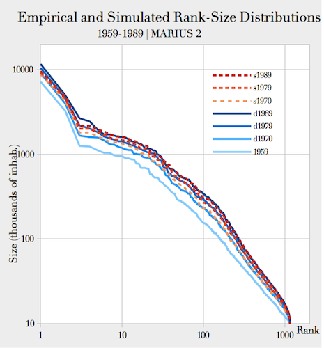
Figure 6. Comparison of empirical and simulated rank-size distribution of cities Table 2: Best calibration of free parameters of MARIUS 2 model Free Parameters Empirical interval Calibrated value \(populationToWealthExponent\) \(> 1\) 1.0866012754 \(sizeEffectOnSupply\) \([ 1; 1.3 ]\) 1.001756388 \(sizeEffectOnDemand\) 1.0792607803 \(economicMultiplier\) - 0.3438093442 \(distanceDecay\) \([ -0.3; 5.2 ]\) 0.6722631615 \(wealthToPopulationExponent\) - 0.3804356044 \(bonusMultiplier\) - 197.9488907791 \(fixedCost\) - 0.2565248068 - 5.5
- The MARIUS model 2 contains a small set of very generic
mechanisms. Yet, it is able to reproduce a very particular pattern: the
evolution of the hierarchical structure of Soviet cities (with
realistic micro-dynamics). This finding supports the main assumption
driving the conception of the MARIUS family of models: namely that it
is possible
for a set of generic core mechanisms to describe cities' interactions
and their influence on the system's structure (independently of the
particular contexts in which these interactions take place). The
calibrated model has four characteristics:
- Wealth is unevenly distributed among cities with respect to their size: larger cities tend to be much richer per capita than smaller ones (\(populationToWealth = 1.09\)).
- This scalar inequality is more pronounced on the consumption side (\(sizeEffectOnDemand > sizeEffectOnSupply\)).
- The effect of distance on the reduction of interaction potential is less important in this large country than in other cases from the literature (\(distanceDecay = 0.67\)).
- The effect of the gain of a certain amount of value on attractivity decreases with city size (\(wealthToPopulationExponent < 1\)).
- 5.6
- Obviously, these generic mechanisms would not simulate appropriately each city's trajectory without particular features added to the model. However, this generic model is an important building block for further investigation of the Soviet system of cities, as well as other systems. We now have to assess the model's degree of parsimony, as it might be that some degrees of freedom resulting from the use of free parameters are useless and the model can be further constrained.
- 5.7
- In order to examine this extent, we will use the
calibration profile
technique (Reuillon et al. 2015)
to deepen our understanding of the free parameters' effect on the model
fitness. Calibration profiles depict the effect of each parameter on
the model behaviour, independently from the variation of the other
parameters. Indeed, each profile exposes the lowest calibration error
that can be obtained as a function of the value of the parameter under
study. Therefore, for each value of the parameter under study, all the
other parameters are optimised by a GA calibration and the lowest
distance to data is plotted on the Y-axis against that parameter value
on the X-axis. It produces 2-dimensional graphs showing the impact of
the parameter under study on the ability of the model to produce
expected dynamics. To ease the interpretation of the profiles, an
acceptance threshold is generally defined. For results lying below the
acceptance
threshold, the calibration error is considered satisfying and the
dynamics exposed by the model acceptable. Figure 7
shows four typical shapes that a calibration profile may take for a
given parameter of a model.
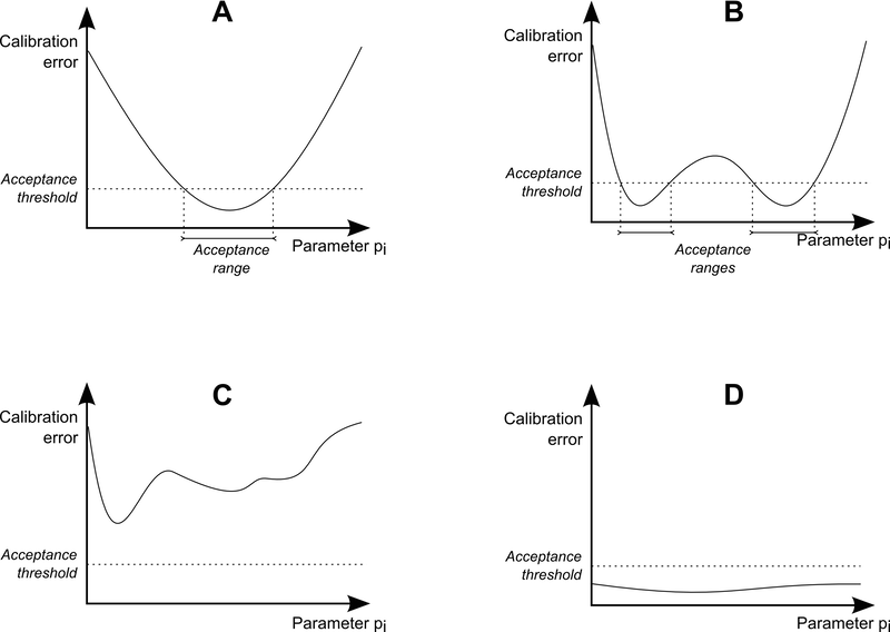
Figure 7. Stylized sensitivity profile shapes - 5.8
- Four shapes have been discriminated:
- Shape A is exhibited when a parameter is restrictive with respect to the calibration criterion. In this case, the model is able to produce acceptable dynamics only for a specific range of the parameter. A connected validity interval can then be established.
- B is observed when a parameter is restrictive with respect to the calibration criterion. However in this case, the validity domain of the parameter is not connected. It means that several qualitatively different regimes of the model meet the fitness requirement. In this case, the model dynamics should be observed directly to determine if the different kinds of dynamics are all suitable or if some of them are mistakenly accepted by the calibration objective.
- The shape C is encountered when the model is impossible to calibrate. The profile does not expose any acceptable dynamic according to the calibration criterion. In this case, the model should be improved or the calibration criterion should be adapted.
- The shape D is encountered when a parameter does not restrict the model's dynamics with respect to the calibration criterion. The model can always be calibrated whatever the value of the parameter is. In this case, the parameter provides a superfluous degree of freedom for the model since its effect can always be compensated by a variation of other parameters. In general, it means that the parameter should be fixed or that the its value should be expressed as a function of other parameters.
- 5.9
- We confirm that the model gives its best results when the scaling exponents are above and close to 1, that is, in the empirical range expected from the literature on agglomeration economies. For example, a value over 1.7 for \(populationToWealth\) and over 1.1 for the \(sizeEffects\) on \(Supply\) and \(Demand\) produce a distribution of city sizes very distant from the observed ones in 1970, 1979 and 1989 in the Former Soviet Union. The ranges for \(sizeEffects\) on \(supply\) and \(demand\) are very narrow, and the best results of the model are achieved when the exponent of the scaling law for consumption is higher than the exponent for production.
- 5.10
- The profile of \(economicMultiplier\) shows a range of acceptable values between 0 and 1. It is impossible to set its value over 1 without making the model generate overflows. We can assess its necessity (and subsequently the necessity of exchanges in this model) by noting that the model does not expose acceptable behaviour when \(economicMultiplier\) is set at 0. Indeed, its value should fall in the range \([0.04; 0.67]\).
- 5.11
- The range for the parameter estimating the decreasing
effect of distance on interaction potentials (\(distanceDecay\)) is
acceptable between 0.4 and 1.2. It is once again a value expected from
the literature (Fotheringham
1981; Baccaïni
& Pumain 1998), and a relatively low interval. It
means that distance plays a negative but rather small effect on
interurban interactions in the Soviet space as modeled with MARIUS.
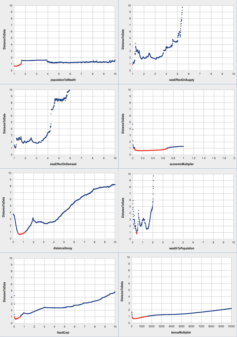
Figure 8. Profiles of MARIUS free parameters
Red dots indicate the sets of parameters leading to a distance to data below our acceptance threshold for this model. We fixed this value at 1, close to the distance of the best calibrated model (0.65) and yet restrictive enough. - 5.12
- The most interesting result is obtained with the less documented parameter, \(wealthToPopulationExponent\). We do not know empirically if the elasticity between wealth accumulation and population accumulation is increasing or decreasing (meaning respectively a value \(\geq 1\) or \(\leq 1\)). The profile for this parameter shows that both possibilities can result in a simulated distribution of city sizes roughly comparable to that observed in the Former Soviet Union. Yet, the only sets of parameters located below our acceptance threshold indicate a decreasing elasticity: when \(wealthToPopulationExponent\) is close to 0.4. Above 2, the results of the model cannot be satisfying.
- 5.13
- Finally, we show the necessity of the \(bonus\) and \(fixedCost\) mechanisms by showing that the results of the model with a parameter equal to 0 are far from expected, according to our evaluation criteria. The best range for these parameters are between 0.04 and 0.6 for \(fixedCost\) and in the interval \([ 50; 1500 ]\) for \(bonusMultiplier\).
- 5.14
- All parameters and associated mechanisms were shown necessary to the dynamics of Model 2 through the sensitivity analysis of profiles, suggesting that the complexification of the model is not necessary for the reproduction of the expected structure of the Soviet system of cities between 1959 and 1989.
Conclusion
-
Methodological discussion
- 6.1
- In conclusion, we want to assess our progress in the understanding and prediction of the Soviet system of cities' evolution. When trying to reproduce the stylised facts characterizing systems of cities' evolution in general and the observed trajectory of the Soviet one between 1959 and 1989, we produced two parsimonious agent-based models and two ways of evaluating them. This progressive process of model-building and evaluation may seem time-consuming, but it shows very interesting results:
- 6.2
- We first showed the trade-off between model complexity and the level of requirements of its output. Macro-regularities have been reproduced via a simple model of interurban exchanges (Model 1), although the micro-dynamics generating them were not realistic. By adding some knowledge in the evaluation function and thanks to an extensive experiment campaign, we showed that Model 1 was unable to produce realistic dynamics and macro regularities at the same time. The limit of Model 1's expressivity has been reached. No satisfying behaviour was found with such constraints.
- 6.3
- By adding two mechanisms to Model 1, the range of Model 2's
possible behaviours were extended satisfactorily, as revealed by
calibration (section 5). Thus,
the complexity increment between Model 1 and Model 2 is justified both
theoretically and experimentally. Moreover, we see in Figure 9 that those simple models better
simulate the distribution of city sizes than the most famous growth
model (Gibrat's). This Figure plots the observed and simulated
populations of cities sorted by size for all three calibrated MARIUS
models presented earlier, and the median results of 100 replications of
a Gibrat's model based on successive empirical growth rates. We see
that Gibrat's simulations tend to under-estimate the growth of all
cities in the Former Soviet Union. On the contrary, the MARIUS models
get
very close to the empirical distribution, and the more refined model
structure, the closer it fits the historical data.
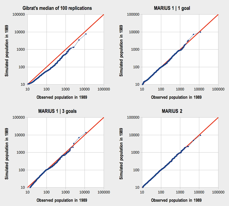
Figure 9. Comparative evaluation of models' outputs
Blue dots indicate the projection of simulated against observed populations of cities sorted by size in 1989. They would be aligned on the red line if the model predicted the exact distribution of city sizes. - 6.4
- Methodologically speaking, explicitly relating the process
of model-building and model evaluation enables to expose some dead-ends
and especially to justify areas of complexification
of a model that we tried to keep as parsimonious as possible. We found
that such an abductive method (EBIMM) helps generate macro structures
comparable to empirical regularities, while injecting theoretical
meaning into the modelled hypotheses. We also believe that such a
method is a possible way of filling the gap between KISS and KIDS
approaches in a progressive, experimentally justified and reproducible
way. Moreover, starting the design of the MARIUS grid from the most
general mechanisms ensures their reusability in modelling other systems
of
cities, since the low-level blocks of the model are not specific to the
target system.
Main geographical findings and perspectives
- 6.5
- The application of this method to the case of the Soviet system of cities between 1959 and 1989 has shown that generic processes of interaction and uneven distributions of wealth and productivity were sufficient to simulate the evolution of the Soviet city system's hierarchy. This supports the evolutionary theory of systems of cities by identifying one possible set of generic mechanisms that could apply to other systems of cities. Moreover, we found that exchanges and interactions were at the core of the cities differentiation, because a model without spillover effects (Model1) was not able to reproduce this hierarchy and hierarchisation process. Finally, the sensitivity analysis helped explore two qualitative regimes for the elasticity parameter \(wealthToPopulation\), which would be hard to evaluate with empirical data. Finally, the results obtained with the second model are closer to the observed data than stochastic models such as Gibrat's are.
- 6.6
- The main feature of this approach is to complexify the evaluation and the model in parallel. At this point, we find a good fit of the model to empirical regularities at a macro-geographical scale. An investigation of the micro-geographic trajectories of cities would suggest that such a simple model is unable to simulate the location and distribution of growth in the system. An easy way to measure the distance to empirical trajectories would be to measure the distance between simulated and observed populations of individual cities (instead of their distribution sorted by size). This exploration could reveal the need for new mechanisms (for example localised resource extraction or fiscal redistribution) which provide greater realism at a meso-level of inquiry. This is the direction of our current work.
Acknowledgements
- We thank the three anonymous referees for their constructive remarks, Denise Pumain for stimulating and overviewing this project, Robin Morphet for a final proof-reading, and funding institutions which made this project feasible : University Paris 1 Panthéon-Sorbonne, the Complex Systems Institute in Paris (ISC-PIF) and the ERC Grant GeoDiverCity.
Notes
-
1
Models of Agglomerations in the perimeter of Imperial Russia and the
Soviet Union
2 Emergence is understood here as the "weak" emergence of a higher level structuration unexpectedly regular, resulting from the lower level behaviour of cities and their interactions (Batty 2006; Pumain 2006) rather than its "strong" meaning of a creation "not deducible even in principle from truths in the low-level domain" (Chalmers 2006, p.244).
3 DARIUS database describes 1929 cities in the post-Soviet space, from census figures aggregated using a definition of cities as morphological units of more than 10.000 inhabitants, available here: http://dx.doi.org/10.6084/m9.figshare.1108081
4 https://github.com/ISCPIF/marius-method
5 "Theory can explain the Russian trends when they are not deeply distorted by some extraordinary events, which, however, were and are so common in this country" (Nefedova & Treivish 2003, p.75)
6 This temporal increment is common to most urban growth models. It seems to be precise enough to represent consistent interurban interactions, yet commensurable with the empirical time scale of censuses produced every ten years or so.
7 For a discussion of the suitability of using concepts such as wealth and agglomeration economies in the Soviet case, see box 1.
8 For consistancy with equations 3 and 4, the wealth gain is divided by \(economicMultiplier\).
9 N.B.: Prior to computing the difference between the log of their population, cities are sorted according to their population
11 https://github.com/ISCPIF/marius-method/tree/master/openmole
12 https://github.com/openmole/mgo
13 The best possible model would have no city without wealth, a nil totalOverflowRatio and the same distribution of city sizes as the empirical one for each census.
14Note that satisfactory values for the closeness-to-data objective have been found (around 2.7), but they expose infinite values for the overflow objective. These solutions have not been represented in Figure 5.
References
- ALLEN, P. M., & Sanglier,
M. (1981). Urban evolution, self-organization, and decisionmaking. Environment
and Planning A, 13(2), 167–183.
AMBLARD, F., Bommel, P., & Rouchier, J. (2007). Assessment and validation of multi-agent models. In F. Amblard & D. Phan (Eds.), Multi-Agent Modelling and Simulation in the Social and Human Sciences (pp. 93–114).
BACCAÏNI, B., & Pumain, D. (1998). Les migrations dans le système des villes françaises de 1982 à 1990. Population (french edition), 53(5), 947–977.
BATTY, M., & Torrens, P. M. (2001). Modeling complexity: the limits to prediction. Cybergeo: European Journal of Geography, 201.
BATTY, M. (2006). Hierarchy in cities and city systems. In D. Pumain (Ed), Hierarchy in natural and social sciences (pp. 143–168). Springer Netherlands.
BATTY, M. (2007). Cities and complexity: understanding cities with cellular automata, agent-based models, and fractals. The MIT press.
BATTY, M. (2011). Cities, prosperity, and the importance of being large. Environment and Planning B: Planning and Design, 38(3), 385–387.
BATTY, M., Crooks, A. T., See, L. M., & Heppenstall, A. J. (2012). Perspectives on agent-based models and geographical systems. In J.A. Heppenstall, A.T. Crooks, L. M. See & M. Batty (Eds.), Agent-Based Models of Geographical Systems (pp. 1–15). Springer Netherlands.
BETTENCOURT, L. M., Lobo, J., & West, G. B. (2008). Why are large cities faster? Universal scaling and self-similarity in urban organization and dynamics. The European Physical Journal B-Condensed Matter and Complex Systems, 63(3), 285–293.
BETTENCOURT, L. M., Lobo, J., & West, G. B. (2008). Why are large cities faster? Universal scaling and self-similarity in urban organization and dynamics. The European Physical Journal B-Condensed Matter and Complex Systems, 63(3), 285–293.
BRETAGNOLLE, A., Daudé, E., & Pumain, D. (2006). From theory to modelling: urban systems as complex systems. Cybergeo: European Journal of Geography, 2420.BRETAGNOLLE, A., Pumain, D., & Vacchiani-Marcuzzo, C. (2009). The organization of urban systems. In D. Lane, D. Pumain, S. Van der Leeuw & G. West (Eds.), Complexity perspectives in innovation and social change (pp. 197–220). Springer Netherlands.
BRETAGNOLLE, A., & Pumain, D. (2010). Simulating urban networks through multiscalar space-time dynamics: Europe and the united states, 17th-20th centuries. Urban Studies, 47 (13), 2819-2839.
BURA, S., Guérin-Pace, F., Mathian, H., Pumain, D., & Sanders, L. (1996). Multiagent systems and the dynamics of a settlement system. Geographical analysis, 28(2), 161–178.
CASTELLS, M. (1996). The information age: economy, society and culture. Vol. 1, The rise of the network society (Vol. 1). Oxford: Blackwell.
COASE, R. H. (1937). The nature of the firm. Economica, 4(16), 386–405.
CICCONE, A., & Hall R. E. (1996). Productivity and the density of economic activity. American Economic Review, 86(1), 54–70.
CHALMERS, D. J. (2006). Strong and weak emergence. In. P. Clayton & P. Davies (Eds), The reemergence of emergence (pp. 244–256) Oxford University Press.
CHISTALLER, W. (1933). Central Places in Southern Germany. Translation into English by Carlisle W. Baskin in 1966.
COMBES, P. P., & Lafourcade, M. (2012). Revue de la littérature académique quantifiant les effets d'agglomération sur la productivité et l'emploi. http://www.parisschoolofeconomics.com/lafourcade-miren/SGP.pdf
COTTINEAU, C. (2014). L’évolution des villes dans l’espace post-soviétique. Observation et Modélisations. PhD Dissertation. University Paris 1 Pathéon-Sorbonne.
COTTINEAU, C. (2013). An intermediate systemTrajectories of Russian cities between general dynamics and specific histories. L'Espace géographique (English Edition), 41(3).
DURANTON, G., & Puga, D. (2004). Micro-foundations of urban agglomeration economies. Handbook of regional and urban economics, 4, 2063–2117.
EPSTEIN, J. M., & Axtell, R. (1996). Growing artificial societies: social science from the bottom up. Brookings Institution Press.
FOTHERINGHAM, A. S. (1981). Spatial structure and distance-decay parameters. Annals of the Association of American Geographers, 71(3), 425–436.
FRENCH, R. A., & Hamilton, F. I. (Eds.). (1979). The socialist city: Spatial structure and urban policy. John Wiley & Sons.
FUJITA, M., & Thisse, J. F. (1996). Economics of agglomeration. Journal of the Japanese and international economies, 10(4), 339–378.
GANG, I. N., & Stuart, R. C. (1999). Mobility where mobility is illegal: Internal migration and city growth in the Soviet Union. Journal of Population Economics, 12(1), 117–134.
GIBRAT, R. (1931). Les inégalités économiques. Paris: Librairie du Recueil Sirey.
GLAESER, E., Kallal, H., Scheinkman, J. A. & Shleifer A. (1992). Growth in cities. Journal of Political Economy, 100(6), 1126–1152,
GRIMM, V., Berger, U., Bastiansen, F., Eliassen, S., Ginot, V., Giske, J., ... & DeAngelis, D. L. (2006). A standard protocol for describing individual-based and agent-based models. Ecological modelling, 198(1), 115–126.
GRIMM, V., & Railsback, S. F. (2012). Pattern-oriented modelling: a 'multi-scope' for predictive systems ecology. Philosophical Transactions of the Royal Society B: Biological Sciences, 367(1586), 298–310.
HARRIS, C. D. (1970). Cities of the Soviet Union, Studies in their Functions, Size, Density and Growth. Chicago: Assciation of Amercian Geographers.
HENDERSON, J. V. (1986). Efficiency of resource usage and city size. Journal of Urban economics, 19(1), 47–70.
HEPPENSTALL, A. J., Crooks, A. T., See, L. M., & Batty, M. (Eds.). (2012). Agent-based models of geographical systems. Springer Science & Business Media.
IYER, S. D. (2003). Increasing unevenness in the distribution of city sizes in Post-Soviet Russia. Eurasian Geography and Economics, 44(5), 348–367.
KHOREV, B.S. (1975). Problemy gorodov: urbanizaciya I edinaya sistema raseleniya v SSSR. 'Musl'.
LAPPO, G. M., & Polian, P. M. (1999). Rezultaty Urbanizacii v Rossii k koncu XX veka. Mir rossii, 4, 35–46.
MANOVE, M. (1971). A model of Soviet-type economic planning. The American Economic Review, 390–406.
MARSHALL, A. (1890). Principles of Economics. Macmillan. London.
NEFEDOVA, T., & Treivish, A. (2003). Differential urbanisation in Russia. Tijdschrift voor economische en sociale geografie, 94(1), 75–88.
NEUBERGER, E. (1968). The Legacies of Central Planning (No. RAND-RM-5530-PR). RAND Corp Santa Monica CA.
PIKETTY, T. (2013). Le capital au XXIe siècle. Seuil.
PUGA, D. (2010). The Magnitude and Causes of Agglomeration Economies. Journal of Regional Science, 50(1), 203–219.
PUMAIN, D. (1997). Pour une théorie évolutive des villes. Espace géographique, 26(2), 119–134.
PUMAIN, D. (Ed) (2006). Hierarchy in Natural and Social Sciences. Springer
PUMAIN, D., & Sanders, L. (2013). Theoretical principles in inter-urban simulation models: a comparison. Environment and Planning A, 45(9), 2243–2260.
PUMAIN, D., Swerts, E., Cottineau, C., Vacchiani-Marcuzzo, C., Ignazzi, A., Bretagnolle, A., Delisle, F., Cura, R., Lizzi, L. & Baffi, S. (2015). Multilevel comparison of large urban systems. Cybergeo: European Journal of Geography.
RAVENSTEIN, E. G. (1885). The laws of migration. Journal of the Statistical Society of London, 167–235.
REUILLON, R., Schmitt, C., De Aldama, R. & Mouret, J.-B. (2015). A New Method to Evaluate Simulation Models: The Calibration Profile (CP) Algorithm. Journal of Artificial Societies and Social Simulation, 18(1).
SANDERS, L., Pumain, D., Mathian, H., Guérin-Pace, F., & Bura, S. (1997). SIMPOP: a multiagent system for the study of urbanism. Environment and Planning B, 24, 287–306.
SANDERS, L. (2001). Modeles en analye spatiale: introduction. Modèles en analye spatiale, 17–29.
SANDERS, L. (2007). Agent models in urban geography. Agent-Based Modelling and Simulation in the Social and Human Sciences. In F. Amblard & D. Phan (Eds.), Multi-Agent Modelling and Simulation in the Social and Human Sciences (pp. 174–191).
SCHMITT, C., Rey-Coyrehourcq, S., Reuillon, R. & Pumain D. (2015) Half a billion simulations: evolutionary algorithms and distributed computing for calibrating the SimpopLocal geographical model. Environment and Planning B, advance online publication, [doi://dx.doi.org/10.1068/b130064p]
SIMON, H. A. (1955). A behavioral model of rational choice. The Quarterly Journal of Economics, 99–118.
SNYDER, T. (1993). Soviet monopoly. In J. Williamson (Ed), Economic Consequences of Soviet Disintegration, (pp. 176–243).
SPULBER, D. F. (2007). Global competitive strategy. Cambridge University Press.
THIELE, J. C., Kurth, W., & Grimm, V. (2014). Facilitating Parameter Estimation and Sensitivity Analysis of Agent-Based Models: A Cookbook Using NetLogo and 'R'. Journal of Artificial Societies and Social Simulation, 17(3), 11 https://www.jasss.org/17/3/11.html
XU, Z. (2009). Productivity and agglomeration economies in Chinese cities. Comparative Economic Studies, 51(3), 284–301.
ZIPF, G. K. (1949). Human behavior and the principle of least effort. Cambridge (Mass.), Addison-Wesley Press.