
 Abstract
- This article describes a scalable way to initialise a simulation model with correlated random numbers. The focus is on the nontrivial issue of creating predefined multidimensional correlations amongst those numbers. A multi-agent model serves as a basis for practical demonstrations in this paper, while the method itself is interesting for an even wider audience within the modelling and simulation community beyond the field of agent-based modelling. In particular, we demonstrate how streams of correlated random numbers for different empirically-based model parameters can be generated when just given aggregated statistics in the form of a correlation matrix. An example initialisation procedure is demonstrated using the open source statistical computing software "R" as well as the open source multi-agent simulation software "Repast Simphony" We also provide a digression for NetLogo users.
- Keywords:
- Correlated Random Numbers, R-Project, Repast, Guide, Tutorial
Introduction
- 1.1
- The simulation of a model may sometimes require setting many parameters which influence its outcome. In a subset of these cases, the parameters may be interdependent in such a way that the initialisation of a model needs two or more parameters to correlate in a predefined manner. A procedure to generate and utilise such numbers will be explained in the following. We use the example of an agent-based model, since one of our main research areas is the field of agent-based economics. In this research, we regularly find scenarios to which the concept presented in this contribution is applicable. During this paper, an illustrative example will be used to explain our central ideas in the context of multi-agent simulations. However, the concept can easily be transferred to the initialisation of other types of simulation models as well.
- 1.2
- In a variety of multi-agents systems, the model to be simulated may consist of a large number of heterogeneous agents. Heterogeneity can come in the form of different spatial positions of individual agents, different network connections, opinions, etc. In general, each of these agents possesses a set of parameters with different initialisation values. Researchers may want to relay data acquired from the real world (e.g. through measurement series, questionnaires or statistical archives) to initialise their agents with according parameter values for reasons of testing, forecasting, or simply for validity.
- 1.3
- In the case of social or economic simulations, agents may possess variables such as income, reputation, job satisfaction, household size, etc. One may however not in all cases be lucky enough to find real-world-data at a level that is as detailed as their desired simulation setup may require. A possible option is to evade to more aggregated forms of simulation, matching the aggregation level of the empirical data available. This option can be unsatisfactory as important details of the micro-level to be simulated and/or the emerging micro-macro-links within such a simulation might need to stay unaddressed.
- 1.4
- In the remainder of this paper we are adressing an alternative way to cope with such data limitations. In the course of our approach we assume that aggregated distributions and correlations of different variables are given in an empirical study even though more detailed data is not available. Still we aim for a simulation at a detailed level (exploring the dynamics of interaction between individuals) that takes into account the empirical facts.
Demonstrative example
- 2.1
- In the course of this paper we will use a fictitious example to explain our ideas. More specifically, a social network of historical painters is to be simulated using multiple agents. Let us assume that in the past an empirical study on these painters was conducted that analysed for several painters in each year the quality of their works, sales prices as well as the age of the painters and their ability to attract painting apprentices. Let us further assume that unfortunately the detailed data revealed during this study were lost or never got published. However, aggregated results in the form of a correlation matrix, as given in table 1, are still available. This situation that only aggregated data is published can be viewed as typical for many empirical studies, for instance in organizational research (e.g. Oreg 2006) that is of particular interest to us.
Table 1: Correlation matrix between parameters of a fictitious painter agent (demonstrative example) Variable Mean Standard
Deviation1 2 3 4 1. Age 40 12 1 0,4 0,6 0,6 2. Quality of Paintings 0,7 0,2 0,4 1 0,8 0,4 3. Expected Price of Painting 2000 500 0,6 0,8 1 0,1 4. Educational Reputation 1 0,3 0,6 0,4 0,1 1
- 2.2
- Even though only aggregated correlation data is accessible we desire to simulate individuals in their interaction. In particular, we want to simulate where painters become apprentices and how this influences their later success in terms of sales prices, quality of work and attractiveness as a teacher to other painters. A multi-agent simulation on the micro-level of individuals, based on the (static) aggregated correlation matrix, will allow us to analyse the dynamic behavior in the network of painters.
- 2.3
- In this example, the goal of research in the field of multi-agent-based simulation (MABS) would be to better understand the process of individual and group interaction as well as possible emergent interaction patterns at the macroscopic level of the simulation. Beyond our concrete example there is a broad application potential for performing simulations by using data of published aggregated field studies1. This requires (here: agent-based) modelling at a more detailed level than the aggregated statistical data from such empirical studies provides. To this end we can however use values such as the ones given in our example table 1 to yield specific initialisation data for any number of simulated individuals. This challenge is trivial only when one needs to generate two correlated series of random numbers, i.e. when the agents in the simulation only possess pairs of two correlated properties. In our case here and the way it is often in reality not only two but at least four quantities, e. g. age and quality of pictures, are correlated and connected among themselves, which makes it more difficult to gain individual parameter values for every single agent. In the following we illustrate the necessary procedure by using the mentioned example data.
- 2.4
- The focus on correlations in the steps we describe here shows a similarity to factor analysis. However, while factor analysis aims for data reduction (either in the variables or, less common perhaps, in the persons/entities) our method aims to reconstruct (and then simulate) the detailed level of individuals from aggregated correlation data. Thus, one could call the approach something like the reverse of a factor analysis.
Mathematical Background
- 3.1
- For only two numbers (parameters) to be correlated, there is a simple approach to derive two correlated random numbers from a set of uncorrelated random numbers:
y1 =  *x1
*x1(1) y2 = c*  +
+  **x2
**x2(2)
where x1 and x2 are two uncorrelated random numbers from a given distribution, and
and  are their standard deviations, and c is the desired correlation coefficient between y1 and y2; i.e. the resulting correlated random numbers.
- 3.2
- With more than two sequences of correlated random numbers to generate, one can use a variety of mathematical approaches that are more or less difficult to go through manually. In our case, an Eigenvector-decomposition was employed. There also is the option of using the Cholesky-decomposition (Trefethen & Bau III 1997, pp. 172–178) which will however not be explained further here. Given a correlation matrix C (see table 1) one can define a matrix
V = EiDiag 
(3) - 3.3
- where Ei are the eigenvectors of C and
 are the eigenvalues of C.
With a matrix Iu consisting of formerly uncorrelated random numbers, we can derive a matrix
where VT is the transpose of V. Ic then contains random numbers with correct correlations. Iu can consist of any number of random values where each line can represent the initialisation values for a single agent and each column stands for one of the correlated parameters of an agent. This offers great flexibility since one only needs to choose the number of rows in the original matrix Iu as big as the number of agents one wishes to instantiate/simulate. Iu should not yet include the general distribution properties such as - in our case - the mean and standard deviations given in table 1. These will later be applied to Ic containing the already correlated values. Further details concerning these mathematical fundamentals and the procedure can be found e. g. in (Van den Berg 2012).
are the eigenvalues of C.
With a matrix Iu consisting of formerly uncorrelated random numbers, we can derive a matrix
where VT is the transpose of V. Ic then contains random numbers with correct correlations. Iu can consist of any number of random values where each line can represent the initialisation values for a single agent and each column stands for one of the correlated parameters of an agent. This offers great flexibility since one only needs to choose the number of rows in the original matrix Iu as big as the number of agents one wishes to instantiate/simulate. Iu should not yet include the general distribution properties such as - in our case - the mean and standard deviations given in table 1. These will later be applied to Ic containing the already correlated values. Further details concerning these mathematical fundamentals and the procedure can be found e. g. in (Van den Berg 2012).Ic = IuVT (4)
A Pracitcal guide for the utilisation of correlated random number sequence using "R" and "REPAST"
- 4.1
- While the pattern to generate correlated random numbers shown in section 2 can be time-consuming to do by hand, it is a very easy process once one employs supporting software. The popular and well-documented open source program "R" (Vinod 2009; Jones et al. 2012) is able to make the necessary calculations (for all practical purposes implied here) in just a fraction of a second. The tool, along with many additional packages, can be downloaded freely for a variety of platforms (R 2010).
- 4.2
- Below, we will present exemplary step-by-step R code to generate random number sequences for the four correlated (normalized) parameters "Age", "Quality of Paintings", "Expected Price per Painting", and "Reputation as Educator" listed in table 1. The code is to generate correctly correlated random numbers for 500 agents as virtual "painters". Note that the code pattern is scalable to a very large number of parameters and agents.
- 4.3
- The first step is to generate a matrix filled with uncorrelated random numbers for each agent and parameter.
//Create a matrix with 4 columns for 4 parameters and 500
//rows for 500 agents.Fill data with 500*4 = 2000 random
//values using a normal distribution for all parameters:
Iu <- matrix(data=rnorm(2000), ncol=4, nrow=500)
- 4.4
- Next, the correlations for these parameters need to be filled into another matrix C:
//Create a squared matrix and fill in the correlations
//for each of the four correlated parameters, using the
//order "Age", "Quality of Paintings", "Expected price",
//and "Reputation as Educator":
C <- matrix(, ncol=4, nrow=4)
C[1,] <- c(1,   0.4, 0.6, 0.6)
C[2,] <- c(0.4, 1,   0.8, 0.4)
C[3,] <- c(0.6, 0.8, 1,   0.1)
C[4,] <- c(0.6, 0.4, 0.1, 1)
- 4.5
- R offers a simple command to calculate both the eigenvalues and eigenvectors of a matrix. We will save the result of this operation in an object E. The parameter "symmetric" refers to C being a symmetrical matrix so that only the lower triangle of the matrix needs to be used in the calculations:
E <- eigen(C, symmetric=TRUE)
- 4.6
- The call to
E$vectors will then give us the eigenvectors of C and E$values will return the eigenvalues accordingly. We use the command "diag" to construct a fictive matrix diagonal from the square roots of the three eigenvalues of C. This call is necessary for a valid multiplication. Note that for the calculation of the square roots to be valid, all eigenvalues of C must be positive. This will however implicitly be the case for valid correlation matrices. We can then create the matrix V according to equation 2 given in section 3:
V <- E$vectors diag(sqrt(E$values))
- 4.7
- We can now multiply our formerly uncorrelated random number matrix Iu with the transpose of V in order to receive a matrix Ic with 500 rows each containing correctly correlated values in four columns, where (in our example) the first column stands for the parameter "Age", the second for "Quality of Paintings", the third is for "Expected price per painting" and the last one for "Reputation as Educator":
Ic <- Iu %*% t(V)
- 4.8
- Finally, we must apply the distribution of each parameter (mean and standard deviation) to the correlated random values by simply multiplying each column with the standard deviation and adding to it, the mean of the parameter:
//Apply mean and standard deviation for "Age",
Ic[,1] <- Ic[,1]*12 + 40

//for "Painting Quality",
Ic[,2] <- Ic[,2]*0.2 + 0.7

//for "Expected Price of Painting",
Ic[,3] <- Ic[,3]*500 + 2000

//and finally for "Reputation as Educator"
Ic[,4] <- Ic[,4]*0,3 + 1
- 4.9
- The result of this code can be saved in a CSV-File. In order to do this, we can use the "write.table" command included in R. "write.table" takes several parameters of which the first is the matrix to write into a file and the second is the file's name on disk. The parameter "sep" defines a character by which the values of the matrix are to be separated in the output file. We use "col.names=FALSE" and "row.names=FALSE" to specify that we do not wish to export any column or row names. In order to not put any values of the matrix in quotes, we set "quote=FALSE". In case a value is not set in the matrix (which, following the aforementioned steps, ought to be irrelevant in our case), we can specify a string value written to the file in its place. Here, for instance, we could use the Java-compatible "NaN" string for "not a number" by setting the parameter "na" accordingly:
write.table(Ic,"C:/filename.csv", sep=",", col.names=FALSE,
row.names=FALSE, quote=FALSE, na="NaN")
- 4.10
- We can now use the random number sequences in this file for use in any external program, in our case the Recursive Porous Agent Simulation Toolkit Repast Simphony (North et al. 2006) . It is a Java-based open source software with seemingly growing popularity in the MABS-research community (Barnes & Chu 2010) and is available as a free download (Repast 2010).
- 4.11
- Repast employs a so-called Context Creator to initialise simulations. Within this class, agents can be created and parameters may be set before the simulation begins. Skipping over most of the code of our initialisation routine, we will again present exemplary code to assign the generated correlated values to each agent using the Context Creator, recently also called "SimBuilder". In our example, we wish to create a virtual world with 500 painters, each having different, but correlated parameters as explained above. We utilise a CSV-reader class that simply returns the matrix saved by R as a two-dimensional Java Double array2.
Double[][]correlatedRandomNumbers = CSV_Reader.readFile("C:/filename.csv"); - 4.12
- All we then need to do is to create our agents and read out the correlated random values in the correct order:
//stylised iteration: for (int i=0; i<500; i++) { AgentPainter aP = new AgentPainter(); aP.Age = correlatedRandomNumbers[i,0]; aP.PaintingQuality = correlatedRandomNumbers[i,1]; aP.SellsFor = correlatedRandomNumbers[i,2]; aP.EducationQuality = correlatedRandomNumbers[i,3]; ... } - 4.13
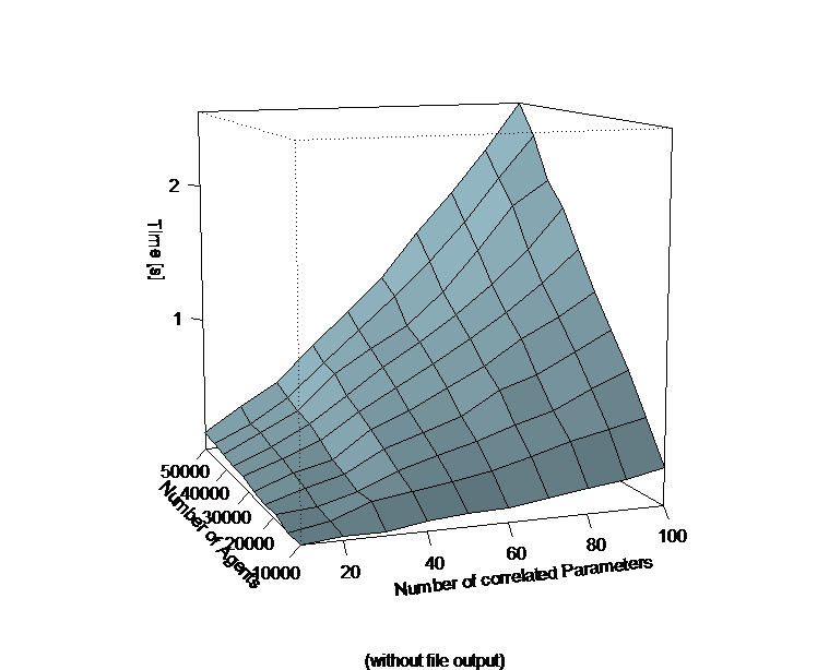
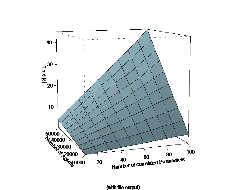
- The approach itself is very flexible and scalable to a large number of agents and correlated parameters. Performance tests were conducted on an Intel Core2-Duo PC with 4GB memory and a hard disk spinning at 5400rpm. Figure 1 shows a 3D-mesh-plot portraying the execution times for the generation of 10.000 to 50.000 correlated vectors (i.e. agents) for respectively 10 to 100 parameters for each individual. The left part of figure 1 displays execution times for the calculations themselves without disk output to a CSV file. The righthand plot shows execution times including the disk output. The data shows that even for the calculation of 100 correlated parameters for 50.000 agents it only takes slightly over two seconds to retrieve all necessary values using a code analogous to the example code listed above. Also, the computation complexity seems to rise only linearly with a rising number of agents and parameters which makes this approach interesting for large scale simulations with either a large number of agents or parameters in one simulation, or a large number of simulations running in parallel (e.g. for parameter optimisation purposes).
- 4.14
- Note that there is, however, a performance-bottleneck where the files need to be written to disk. Thus, it would be helpful to not read in the data necessary for initialisation from a file, but to send the commands necessary directly from the simulation tool to R and to then evaluate the results. In addition it could also be possible that in the case of a multi agent simulation particular agents are not generated and initialized at the beginning of a simulation, but come into being during the running process. Here you cannot be sure about the date of origin or the availability of a CSV file mentioned above. Transferred to our fictitious example of the painters this could mean that after a first initialisation we would like to grow the painters older with every time step of the simulation. Additionally individuals shall leave the simulation due to retirement and others join because of first-time employment. On the assumption that the correlations have to be valid for the progressing simulation, too, in every time step all parameters have to be calculated anew. This makes the so far procedure of saving the results in R and importing them from files impractical. In addition the usage of files would make the simulation much slower in every calculation step.
Sending R Commands directly from Repast
- 5.1
- Therefore, one should refer to (Lang 2005) or (JRI 2013) for a way to directly call R-functions from within Java- based applications such as Repast. We will explain this process briefly in the following.
- 5.2
- The so-called Java-R-Interface (JRI 2013), amongst other interfaces available, is able to send commands to an instance of R running in the background of a Java-based application. Since simulations in the MAS-tool Repast Simphony can be programmed in the Java language, JRI can be easily implemented for use in such multi-agent-simulations.
- 5.3
- JRI is available as part of a package-extension of R called "rJava", which was originally designed to send data and commands in the opposite direction, i.e. from R to Java. The quickest method to utilise only the functionality of the Java-R-Interface, nevertheless, is to install the complete "rJava" package within R. Once installed, the downloaded folders within R's own extension library will contain the JRI Java-archive for implementation as a library in any Java project, too. 3 Once JRI is available for use in Repast, one can extend the initialisation class of a simulation analogously to the case of CSV files described above. However, here one would directly initialise agents using the calculations made in R. For our example case, the necessary code is listed below:
- 5.4
- As a first step, it is important to make the JRI library available to the Repast simulation project and include it in the import statements of the simulation part needing to access R, i.e. the ContextCreator.java (or in case one wishes to use the new ReLogo edition: SimBuilder.groovy resp. UserObserver.groovy) class file in our case:
import org.rosuda.JRI.REXP;
import org.rosuda.JRI.Rengine;
import org.rosuda.REngine.*;
- 5.5
- We are then using the initialisation routine of the Context Creator class (e.g. the "build ()" method) to access R routines. Here, we instantiate an object of type Rengine which is the main instance passing commands and data between Java and R. The constructor of this class can pass various arguments to the instance of R to be used. Please refer to the JRI documentation (JRI 2013) at this point in order to adjust this step for your requirements. In all cases, the "
waitForR()" function of the newly created Rengine object should be called to make sure that the R thread finished its program start sequence before calculations can begin. Not including a call to this method may lead to Java exceptions being raised at this step and the failure of Repast's Context Creator initialisation routine:
//Creating a new instance of R for calculations, //making it a public variable to allow access //from external classes such as agents or datasets: public Rengine re; ... re = new Rengine(new String[]{""}, false, null); //Important: waiting for the R instance //to finish loading: if (!re.waitForR()) { System.out.println("Cannot load R"); } - 5.6
- The Rengine type now offers the method "
eval (Stringcommand )" (amongst numerous others) to execute and evaluate a command passed over to R in the form of a simple string parameter. This method returns an object of type REXP (R expression), which can subsequently be used to output or further interpret results of the command sent via "eval". The following code listing demonstrates several calls to send commands to R analogous to the example R-code already given above. We retrieve the final calculation of matrix Ic within the object ex of type REXP:
//Creating instance for return values: REXP ex; //Executing R example code as stated in //beginning of section 4 of this paper: re.eval("Iu <- matrix(, ncol=4, nrow=500)"); re.eval("Iu[,] <- rnorm(2000); re.eval("C <- matrix(, ncol=4, nrow=4)"); re.eval("C[1,] <- c(1, 0.4, 0.6, 0.6) "); re.eval("C[2,] <- c(0.4, 1, 0.8, 0.4) "); re.eval("C[3,] <- c(0.6, 0.8, 1, 0.1) "); re.eval("C[4,] <- c(0.6, 0.4, 0.1, 1) "); re.eval("E <- eigen(C,symmetric=TRUE)"); re.eval("V <- E$vectors %*% diag(sqrt(E$values))"); //Catching the result of Ic in "ex" for further handling: ex =re.eval("Ic <- Iu %*% t(V)"); - 5.7
- Now we only need to create an array just as one would when using CSV files. The REXP type has several routines for formatting the results, e.g. an "
asString()" method for outputting its contents to the Java console. Here, we use the "
asMatrix()" method that interprets the results as a two-dimensional array of Double values. We can then again use this array to iterate through it, assigning the parameter values to each of our agents:
Double[][] corrRandNumbers=ex.asMatrix() //stylised iteration: for (int i=0; i<500; i++) { AgentPainter aP = new AgentPainter(); aP.Age = corrRandNumbers[i,0] * 12) + 40; aP.PaintingQuality = corrRandNumbers[i,1] * 0.2) + 0.7; ... } - 5.8
- In the above code example we have decided to assign the random numbers directly in the Repast Code, as they are just simple multiplications and additions, for which we do no longer have to use the Java R Interface. Of course one could provide the correlated random numbers by analogy to the code from Section 4 by using further re.eval commands.
- 5.9
- Accessing R through the JRI library is a very efficient method to compute the necessary calculations for the initialisation of a Repast simulation. Further performance tests using this method have shown that there is no loss of performance when using JRI rather than R itself to create large numbers of correlated random values. Performance results are comparable to those shown in the lefthand part of fig. 1.
Correlations during simulation and between agents
- 6.1
- The JRI offers a much broader range of utilizability than the formulations shown in Section 4 and 5. Beyond the simple initialisation at the beginning of the simulation we are able to gain access to R functions at nearly any position of the simulation. This makes it e .g. possible to create correlated random numbers in every time step after initialisation or at certain incidents. In the fictitious example of the simulation of painters the time is progressing and therefore the ageing of the painters could play a role so that in every time step each painter's age is given, but all other variables have to be calculated accordingly. We did not have this possibility with the approach of Section 4, which focussed on initialising the agents before starting the simulation. To realise the respective routines, it is only necessary to - analogous to Section 5 - use the re.eval (...) command in the step() method of an agent being called-up in every time step.
- 6.2
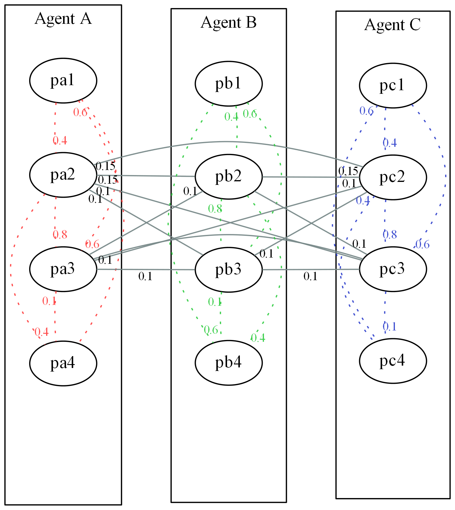
- But another scenario of a similar nature is much more interesting: in our fictitious example the joining painters could during simulation make an introducing training before starting professional life. A number of pupils could visit a painter and probably influence themselves in a limited range during this period of time. We assume that the pupils choose their instructors and that they take into consideration the geographical proximity and the reputation of the painter as an instructor to make their decision. We are interested in the development of local clusters of high and low quality painters or in the spreading of characteristic features during simulation. But first in our fictitious example it is necessary not only to correlate the parameters of each individual agent among each other but also to be able to provide individual parameters of different agents with correlations. Therefore we want to correlate the parameters "Painting Quality" and "Expected Price per Painting" of all pupils of the same painter among each other. Figure 2 shows the constellation of correlation connections for 3 pupils of one agent. It is quickly evident that the correlation connections for a large number of agents and / or correlated parameters lead to a confusing complexity. Finally, for such a calculation, only an extension of a correlation matrix is needed the way it is shown in table 2 for the aforementioned example.
Table 2: Extended correlation matrix for correlations of parameters (1,..,4) within and between agents (a,b,c...) exemplified for the case of 3 agents (see figure 2). For reasons of clarity, only the upper diagonal of the matrix is presented. Var pa1 pa2 pa3 pa4 pb1 pb2 pb3 pb4 pc1 pc2 pc3 pc4 pa1 1 0,4 0,6 0,6 0 0 0 0 0 0 0 0 pa2 1 0,8 0,4 0 0,15 0,1 0 0 0,15 0,1 0 pa3 1 0,1 0 0,1 0,1 0 0 0,1 0,1 0 pa4 1 0 0 0 0 0 0 0 0 pb1 1 0,4 0,6 0,6 0 0 0 0 pb2 1 0,8 0,4 0 0,15 0,1 0 pb3 1 0,1 0 0,1 0,1 0 pb4 1 0 0 0 0 pc1 1 0,4 0,6 0,6 pc2 1 0,8 0,4 pc3 1 0,1 pc4 1
- 6.3
- Theoretically this procedure makes it possible to establish correlation values not only for every single pair of parameters of an agent, but also for every individual pair of parameters between two agents. Transferred to our pupil example this would mean that certain pupils are able to influence each other in particular areas more than other pupils and other areas. For simplification we assume that all pupils influence each other in the same way in the areas mentioned, being shown by the recurring values in the upper right half of table 2. Due to the repetitions this table can be produced dynamically and in a simple manner in Repast for as many pupils as required. We only need to use two interlaced loops to iterate the agent combinations of the upper right half of the correlation matrix through. But beforehand it has to be determined how many agents are the pupils of the painter in question to set up the size of the correlation matrix accordingly. This is done in the step() method of the instructing painter. We assume that a standard network "
networkEduction" of the type Network in Repast has been created and the pupils been placed to the instructors they belong to during the current time step by the command
networkEducation.addEdge(agent,agent)
In the step() method of the instructor we now can fall back on the pupils in the network and create the respective correlation matrix:... //Count pupils of instructing painter: int count_students = networkEducation.getDegree(this); int count_parameters = 4; //Create correlation matrix of corresponding size in R: re.eval("C <- matrix(,ncol=" + (count_students* count_parameters).toString() + ",nrow=" + (count_students* count_parameters).toString()); - 6.4
- Now the correlation matrix can be filled. Due to the simplifications mentioned above only one of the two 4x4 correlation matrices has to be chosen and added, depending on whether it is a correlation between parameters of the same agent or correlations between parameters of different agents. In Repast we differentiate between these two cases and send accordingly adapted
re.eval (...) commands by analogy to Section 5. Here only to the upper right half of the total matrix attention has to be paid, as for further calculations only values above the matrix diagonal have to be used. Herewith the loop construction for filling is further simplified, especially because no symmetrical values below the diagonal have to be produced:
//Iterate through agents vertically and horizontally (this may be simplified if one uses ReLogo): for (int agentV = 1; agentV<=count_students; agentV++) { for (int agentH = agentV; agentH<=count_students; agentH++) { //correlations between paramters of the same agent: if (agentH==agentV) { re.eval("C[" + (agentV-1)*count_parameters + 1 + "," + (agentH-1)*count_parameters + 1 + ":" + (agentH-1)*count_parameters + 4 "] <- c(1, 0.4, 0.6, 0.6) ") ... re.eval("C[" + (agentV-1)*count_parameters + 4 + "," + (agentH-1)*count_parameters + 1 + ":" + (agentH-1)*count_parameters + 4 "] <- c(0.6, 0.4, 0.1, 1) ") //correlations between paramters of different agents: } else { ... re.eval("C[" + (agentV-1)*count_parameters + 2 + "," + (agentH-1)*count_parameters + 1 + ":" + (agentH-1)*count_parameters + 4 "] <- c(0, 0.15, 0.1, 0) ") re.eval("C[" + (agentV-1)*count_parameters + 3 + "," + (agentH-1)*count_parameters + 1 + ":" + (agentH-1)*count_parameters + 4 "] <- c(0, 0.1, 0.1, 0) ") ... } } } - 6.5
- Now a vector of uncorrelated numbers is generated, containing a random value for every parameter of each pupil of the respective agent. Alternatively one could immediately represent this as a matrix with several lines for several groups of agents with equal correlation features and herewith further simplify the code4.
re.eval("cu <- rnorm(" + (count_students*count_parameters).toString() + ")") - 6.6
- Thereafter this vector can be transferred by analogy to the commands in Section 5 to correlated random values and be completed by mean and standard deviations. The results of the example show the parameter values of every individual agent in four columns each, so the columns 1 - 4 contain the values for Agent A, the columns 5 - 8 contain the values for Agent B and the columns 9 - 12 those for Agent C. If you assign these values to the pupils in analogy to the commands from Section 5, now not only the parameter values of an agent are correlated according to table 1, but also the values among the pupils according to the supplementations from table 2.
Excursion: R and NetLogo
- 7.1
- Based on the above-mentioned "rJava" package from which we extracted and used the JRI interface, an extension for NetLogo was developed (Thiele et al. 2012, p. 2.2), (Thiele & Grimm 2010) 5. This NetLogo R extension enables, in a similar manner as sending commands from Repast to R was made possible by JRI, the communication between NetLogo and R. In order to offer example source code also to the large proportion of the NetLogo developers in the JASSS community (cmp. Thiele et al. (2012) fig. 1), we provide a NetLogo template implementation for the required initialization steps during the setup phase of our simulation model at http://www.openabm.org/model/4117/version/1/view. We also provide Repast/Relogo code for the same purpose in an openabm.org model record available from http://www.openabm.org/model/4022/version/1/view.
- 7.2
- The "setup" method of this NetLogo example communicates with R and creates a matrix with 500 rows and 4 columns just as in the Repast examples above. Based on the creation of the correlation matrix and the derived Eigen-vectors and lambda-values, a matrix of correlated parameters Ic is being extracted. Agents are then initialized with these values. A cross-check is then performed by letting R calculate the correlation matrix for the agents' properties. The correlation matrix will be written to the NetLogo console output for comparison with the original correlation matrix.
- 7.3
- In comparison to Repast, however, we cannot simply use a statement like ".asMatrix()" to convert Ic back into a two-dimensional array of numbers. Retreiving Ic from R using
r:get("Ic")will return only a one-dimensional list of values. This is standard behaviour, since arrays and matrices are only available as extensions to NetLogo. Hence, we employ very basic code that is based on the knowledge that there are 500 × 4 values in a particular order in the matrix. The first 500 values in the result list dubbed corrRandNumberswill therefore be age parameters, items 501 to 1000 will contain the values for painting quality, etc.. We are aware that there is room for structural improvements to this code and wish to point out that it is intended for a basic demonstration only. We therefore encourage the audience to make use of the benefits that the above-mentioned extensions may provide to further optimize and parameterize this code in the adaptions you may implement for your own simulations. In addition, while we find that communication between NetLogo and R may be slightly slower than between Repast and R, the NetLogo-R-extension provides additional methods over those in the JRI package such as putList or putAgent, which can provide a way to further optimize your NetLogo simulation models.
Conclusions and extensions
- 8.1
- This article dealt with the question of how to generate scalable sets of correlated random numbers in interaction with agent-based simulations. The authors found this to be a question both important and difficult as many empirical studies provide aggregated descriptive statistics, including correlations, while there is also a necessity for detailed simulations at the level of single and interacting individuals to explore certain issues especially when dealing with complex and/or emergent systems (Nissen & Saft 2010, p. 113). The process of extracting correctly correlated sequences of random numbers for each agent is nontrivial and literature on this topic, especially in the form of practical guides for researchers in the (multi-agent) simulation community without a deep mathematical background, is scarce. The reader therefore was provided with a step-by-step guide for how to create a matrix containing MAS initialisation data in the form of correlated random number sets for each agent as well as with a stylised example code for the wide-spread Repast simulation software in order to access those values indirectly via file output or directly using the so-called JRI-package.
- 8.2
- This paper therefore serves as a demonstrative guide for a wide audience of researchers in the simulation community. It provides a time-saving way as well as a quick access for newcomers to the creation of correlated random number sequences for MAS parameterisation.
- 8.3
- The steps shown here can further be enhanced by using additional packages, e.g. the R-Commander package for R, providing quick and easy access to basic R operations via a graphical user interface (Fox 2010). There are also other options to call R directly from Java and Java-based software (Lang 2005), eliminating the need to use CSV Files for storage. Such approaches are beneficial since one is not only able to outsource initialisation calculations, but any complex set of calculations that should rather be executed in a professional environment such as R.
- 8.4
- An example model demonstrating the basic steps explained in this article in a ReLogo project can be downloaded from http://www.openabm.org/model/4022/version/1/view. Note that this project needs all prerequisites (R, JRI) to be set up and work before it can run correctly.
- 8.5
- This article concentrated on providing a basic, intuitive guide to correctly initialize individual agents from aggregated correlated data. For this purpose, we used the demonstrative example of painters with four, normally distributed, properties. However, one cannot always assume that parameters of similar simulation studies are necessarily normally distributed. They may not even be continuous values, but variables on a categorical/nominal or ordinal scale. The general approach to calculate the initialization values for the agent parameters in R can still be applied in these cases, though. But the R source code required, or the mathematical background, may become less accessible. However, there is useful R code available from some online ressources, also dealing with the statistics of such cases. For instance, in Stevenson (2013) the generation of correlated time series for several categorical parameters by employing additional R packages is demonstrated. To become familiar with the underlying mathematical procedures Gange (1995) can be a helpful source. With these extensions the procedures outlined our paper can be applied in an analogous mode.
Tannenbaum et al. (2006) propose an approximate and even more lean method to simulate correlated categorical and continuous covariates in
the same turn. Using this approach, all parameters of a model are considered to be on a continuous scale and then discretized according to
critical values obtained from correlation information. The authors use the example of simulating virtual patient data for a clinical trial
simulation. However, the idea is not necessarily limited to the example topic. Therefore, the mathematical background provided by former example as well as the
information in Kaiser et al. (2011) regarding the creation of correlated values on an ordinal scale provide ways to extend our approach even further and
may in the future lead to a rich toolset for the community to create simulation models from complex covariate datasets.
Acknowledgements
- The authors would like to thank the anonymous reviewers for their comments and suggestions to improve the quality of the paper, especially with regards to the idea of providing NetLogo source code and very valuable thoughts and literature hints on dealing with categorical variables.
Notes
-
1
We utilise the real-world study of "resistance to change" behaviour in organisations to initialise our own multi-agent simulation of a virtual organisation in order to better understand how resistance to change spreads and can be influenced by management.
2 Several similar Java-based CSV-readers are also available online.
3 Note that the subsequent setup of the JRI library files can be difficult. For a quick overview regarding the most difficult steps in Eclipse/Repast, one can, e.g., refer to easily available short notes and articles in technological blogs such as (Mavlarn 2012) or (StackOverflow 2013).
4 We abandon such simplifications in order to demonstrate the flexibility of our approach.
5 The extension and installation instructions can be downloaded from http://r-ext.sourceforge.net/. Setting up the right combination of your operating system, NetLogo version, NetLogo-R-extension version and R version is a non-trivial, but well-documented process that you will need to follow closely in order to make use of the source code we provide in this section.
References
-
BARNES, D. J. & CHU, D. (2010).
ABMs using Repast and Java.
In: Introduction to Modeling for Biosciences. Springer, pp.
79-130. [doi:10.1007/978-1-84996-326-8_3]
FOX, J. (2010). The r commander: A basic-statistics gui for r. http://socserv.mcmaster.ca/jfox/Misc/Rcmdr/. Archived at: http://www.webcitation.org/6NvGiHhwW.
GANGE, S. J. (1995). Generating multivariate categorical variates using the iterative proportional fitting algorithm. The American Statistician 49(2), 134-138.
JONES, O., MAILLARDET, R. & ROBINSON, A. (2012). Introduction to scientific programming and simulation using R. CRC Press.
JRI (2013). Jri. http://www.rforge.net/JRI/. Archived at: http://www.webcitation.org/6NvIpV2bn.
KAISER, S., TRäGER, D. & LEISCH, F. (2011). Generating correlated ordinal random values.
LANG, D. T. (2005). Calling R from Java. http://www.omegahat.org/RSJava/RFromJava.pdf.
MAVLARN (2012). Calling R from Java using JRI. http://www.cnblogs.com/mavlarn/archive/2012/12/24/2831688.html. Archived at: http://www.webcitation.org/6NvFpp1IE.
NISSEN, V. & SAFT, D. (2010). Social emergence in organisational contexts: benefits from multi-agent simulations. In: Proceedings of the 2010 Spring Simulation Multiconference. Society for Computer Simulation International. [doi:10.1145/1878537.1878548]
NORTH, M. J., COLLIER, N. T. & VOS, J. R. (2006). Experiences creating three implementations of the Repast agent modeling toolkit. ACM Transactions on Modeling and Computer Simulation (TOMACS) 16(1), 1-25. [doi:10.1145/1122012.1122013]
OREG, S. (2006). Personality, context, and resistance to organizational change. European Journal of Work and Organizational Psychology 15(1), 73-101. [doi:10.1080/13594320500451247]
R (2010). The R project for statistical computing. http://www.r-project.org/. Archived at: http://www.webcitation.org/6NvHwxRHI.
REPAST (2010). Repast home page. http://repast.sourceforge.net. Archived at: http://www.webcitation.org/6NvHOTVWA.
STACKOVERFLOW (2013). Question about JRI error. http://stackoverflow.com/questions/4894002/question-about-jri-error. Archived at: http://www.webcitation.org/6NvHgojvH.
STEVENSON, W. (2013). Simulating random multivariate correlated data (categorical variables). http://www.statistical-research.com/simulating-random-multivariate-correlated-data-categorical-variables/. Archived at: http://www.webcitation.org/6NvI7z1VE.
TANNENBAUM, S. J., HOLFORD, N. H., LEE, H., PECK, C. C. & MOULD, D. R. (2006). Simulation of correlated continuous and categorical variables using a single multivariate distribution. Journal of pharmacokinetics and pharmacodynamics 33(6), 773-794. [doi:10.1007/s10928-006-9033-1]
THIELE, J. C. & GRIMM, V. (2010). Netlogo meets R: Linking agent -based models with a toolbox for their analysis .
THIELE, J. C., KURTH, W. & GRIMM, V. (2012). Agent-based modelling: Tools for linking Netlogo and R. Journal of Artificial Societies and Social Simulation 15(3), 8. https://www.jasss.org/15/3/8.html.
TREFETHEN, L. N. & BAU III, D. (1997). Numerical linear algebra, vol. 50. Siam.
VAN DEN BERG, T. (2012). Generating correlated random numbers. http://www.sitmo.com/article/generating-correlated-random-numbers/. Archived at: http://www.webcitation.org/6NvGU3pjH.
VINOD, H. D. (2009). Advances in social science research using R, vol. 196. Springer.