
 Abstract
- In this paper, we survey the use of nowcasting methods in Microsimulation models. These nowcasting methods differ in a number of respects to the more established methods of forecasting. The main distinction is that while forecasting extrapolates from current data to estimate the future, the methods of nowcasting extrapolate from data of the recent past to reflect the present situation. In this paper, we undertake a survey of a number of modelling teams globally, selected for their experience and breadth of use with the methodologies of nowcasting and to ascertain the modelling choices made. Different methodologies are used to adjust the different components, with indexation or price uprating applied for the adjustments to growth in wages or prices, the updating of tax-benefit policy to adjust for policy change and either static or dynamic ageing to account for changes to the population and labour market structure. Our survey reports some of the choices made. We find that these model teams are increasingly utilising variants of these methods for short-term projections, which is relatively novel relative to the published literature.
- Keywords:
- Microsimulation, Survey, Nowcasting, Uprating, Reweighting, Projections
Introduction
- 1.1
- Data used in microsimulation models is typically historic (Callan et al. 2010; Sutherland 2001; Immervoll et al. 2005). This provides an initial constraint for researchers wishing to decompose or estimate the scale and direction of recent changes in the income distribution and in addition for policymakers seeking to monitor such developments. Furthermore, this limits the capacity to provide reliable estimates regarding the direct distributional impact of proposed changes in tax-benefit policies and provides additional challenges for making projections into the future, which can be particularly relevant for analysis relating to the future wellbeing of pension systems.
- 1.2
- As a result, there is a frequent need to update or nowcast data or to project data into the future (see Brewer et al. 2012). The process of nowcasting refers to the estimation of current indicators using data on the past income distribution combined with other current statistics which may include the latest available macroeconomic statistics (Navicke et al. 2013). Nowcasting allows one to better capture, among other things, the impact on the income distribution of a changing population structure from a point in the recent past to the present where there are time lags in the availability of micro data. This contrasts with the more established method of forecasting, which assesses the impact of changes to each income component at some point in the future based on assumptions made about the future.
- 1.3
- The relative success of nowcasting models depends partly on the availability of current aggregate statistics. For example, the rapid changes in labour market status during the recent global economic crisis have important distributional effects (Jenkins and Van Kerm 2014). The ability of nowcasting models to capture these effects depends on the availability of up-to-date aggregate employment statistics. In this paper, we survey a number of modelling teams around the world to investigate how these teams approach the application of nowcasting techniques. We report the choices made and the operational aspects of these choices.
- 1.4
- The nowcasting process can be described in a number of ways.
- Uprating typically refers to issues associated with indexing market income for wage growth.
- Updating may refer to adjusting the tax-benefit rules in a microsimulation model to account for policy change.
- Reweighting or static ageing may apply to changing weights to account for changed population structure, while dynamic ageing refers to simulating changes to the population structure.
- 1.5
- A variety of methods are used for this process. In order to factor in the impact of differential earnings growth and changes in employment, microsimulation models have typically used
- Income uprating parameters to model the impact of differential earnings growth (Immervoll et al. 2005).
- Static ageing or reweighting (Immervoll et al. 2005) to adjust the micro population to account for economic changes.
- 1.6
- However in periods of significant volatility, reweighting may not be appropriate as it may rely excessively on small groups (Klevmarken 1997). In this case, it may be more appropriate to utilise a dynamic income generation model approach to update the data (see Li & O'Donoghue 2014; Bourguignon et al. 2001). There are a number of phases to the study. We undertake a brief literature search of methodologies in section 2. However as the literature is often less clear in terms of some of the methodological choices, we undertook a survey of fifteen model builders, described in section 3. The results of the survey are reported in section 4, with section 5 concluding.
Methodology
- 2.1
- In this section, we describe the methodologies used to update or nowcast in a microsimulation model.
Indexation or Updating
- 2.2
- Redmond et al. (1998) describe the method to index the components of household market income as a process whereby they "pick up our sample in the survey year and parachute it into the modelled year with most survey year demographic and economic characteristics intact, but with incomes and expenditures that reflect changes between the survey year and the policy year." This issue of indexation or updating was listed by Sutherland (2001) as being among six technical problems in the formation of a microsimulation model such as EUROMOD.
- 2.3
- Users face two choices in updating or indexing market income data, namely
- Calibrating levels of income to aggregate national accounts information or
- Updating existing levels of income to account for changes (via indices) in external control totals.
- 2.4
- Correcting for income under-estimation in micro-data is non-trivial (Atkinson et al. 1995) as it can arise due to the non-reporting of income sources, the under reporting of income sources or due to the distribution of the population under-estimating groups in the top one per cent of the income distribution. "Correcting" for this may bias the data more than it is already and it may therefore be more appropriate to leave the distributional incidence of incomes as is and to instead utilise the second approach of updating via indexation by source.
- 2.5
- The next main choice is the degree of disaggregation used in income indexation, which depends partially on the availability of appropriate data to produce indices of average growth rates. These indices are sometimes available by income source and demographic category and are then applied to each income source for each individual to produce a new distribution of household market income.
- 2.6
- Immervoll et al. (2005) evaluated the strengths of various updating methods using micro level indices for most income variables, but in general not differentiated by population sub-group. In terms of the distributional picture, they found that uniform uprating of monetary variables did not reliably capture the real increase in inequality.
- 2.7
- Sometimes indexation is required to correct for differences in the period of analysis. For example, in New Zealand, the period over which income refers to depends upon the year prior to interview. Accordingly the first task of the data preparation is to "synchronise" the data (see Ota & Stott 2007), adjusting the data through indexation to be consistent for the same period of analysis and to "align all of the income and spell information reported by the respondents to a common period". Indexation to later years as described above can then happen.
- 2.8
- While tax-benefit system parametric uprating is a methodological concern in adjusting or updating a micro dataset, it also of policy concern, as differential uprating of these parameters relative to earnings growth can result in fiscal drag in relation to the tax system (Immervoll 2000) and a change in the relative poverty rate relative to the benefit system, via benefit erosion (Hancock et al. 2008).
- 2.9
- Not all income sources or factors that influence income are uprated in the same way. Where the recorded information in the survey includes the mortgage payment as a whole and does not distinguish between the repayment of the mortgage principal and the mortgage interest, the value of mortgage interest must be derived. Updating will then depend upon the type of mortgage payment (see Redmond et al. 1998).
Adjusting for Population Characteristics: Static versus Dynamic Ageing
- 2.10
- We now consider methods to adjust changes to the income distribution due to changes in population characteristics such as demographics, education or labour market characteristics, focusing on two alternative methodologies; adjustment of weights known as static ageing and adjustment of the underlying variables known as dynamic ageing.
- 2.11
- We could also add a third choice, not to adjust for changes to the underlying population, a possible choice given the regular availability of new data in many cases. For example until recently, the published work from the EUROMOD model has concentrated solely on these adjustments for monetary variables, assuming the population structure and labour force status of the underlying population is assumed to remain fixed in the updating of tax-benefit models (Navicke et al. 2013). However where substantial time gaps arise between the availability of micro data, there is a need to update the population characteristics via either static or dynamic ageing.
- 2.12
- Immervoll et al. (2005) describe the process of static ageing or adjusting the weights of the population to correspond to the changes over the relevant period. They define 'static' ageing techniques as methods attempting to align the available micro-data with other known information (such as changes in population aggregates, age distributions or unemployment rates), without modelling the processes that drive these changes (e.g., migration, fertility, or economic downturn). Static ageing thus takes macro-aggregates and then adjusts the underlying distribution to produce projections of the population distribution over time.
- 2.13
- On the other hand, dynamic ageing allows individuals to change their characteristics due to endogenous factors within the model (O'Donoghue 2001). This involves the estimation of a system of econometric equations to simulate changes in the population and monte carlo simulation techniques to replicate the distribution of incomes by sources (Li & O'Donoghue 2014). The dynamic ageing method can be considered as an agent-based method as it models the factors driving the changing characteristics of individual agents over time and does not rely exclusively on trends in statistical aggregates as is the case with static ageing.
- 2.14
- Both methodologies have however some advantages and disadvantages. As such, Pudney (1992) argues that neither approach should be used in isolation. Dynamic ageing by focusing on the agent or individual takes no account of processes at the level of the market such as labour demand. Furthermore, dynamic ageing has huge computational requirements in terms of data and modelling to jointly estimate all the required processes. Dynamic ageing will consistently estimate characteristics of the projected income distribution, under ideal circumstances in which all transitions probabilities and state specific expectations can themselves be estimated consistently. However in a dynamic model, the joint estimation of work and life histories is a formidable requirement given the available data. Therefore, it is necessary to assume that the marginal distributions of different processes are independent (O'Donoghue et al. 2009; O'Donoghue 2010).
- 2.15
- Static ageing has a number of theoretical objections. Firstly, static ageing cannot be used where there are no individuals in the sample in a particular state. If there are a small number of cases of a particular household category, a very high weight may have to be applied, resulting in unstable predictions. Changing demographic and economic trends over time may mean that increasing weight is placed on population types with very few cases in the sample (see Klevmarken 1997). Secondly, static ageing procedures are relatively well suited to short to medium term forecasts where changes in the structure of the population are small. However, over longer periods of time or over more turbulent periods, this is more problematic. In the following, we take a look at some of the efforts being made to minimise the effect that these weaknesses may have on nowcasting or forecasting models.
Adjusting for Population Characteristics: Static Ageing
- 2.16
- Immervoll et al. (2005) describe a static ageing technique known as "re-weighting" (altering the "weights" of different observations in the data) in order to meet control totals for the policy simulation year. It is frequently used where there is a time lag between the data year and the policy simulation year (e.g. Adelzadeh 2001; Flory & Stöwhase 2012).
- 2.17
- Creedy (2003) describes the theory associated with a number of potential reweighting methods, using these to reweight the 2000/2001 wave of the New Zealand Household Economic Survey (HES) data to the 2003/2004 wave of the same dataset. The functions included a chi-square distance function, a modified chi-square distance function and the Deville-Särndal function. As in the case of Immervoll et al. (2005), the distance functions are used to minimise the aggregate distance between the original and new weights while aligning the data to control totals for the simulation year. This allowed the author to analyse distributional changes in tax-benefit expenditures during that particular time.
- 2.18
- Immervoll et al. (2005) generated the re-weighting results by adjusting the sample weights contained in the 1996 wave of the Finnish Income Distribution Survey (IDS) survey to align with control totals derived from the 1998 wave of the same dataset. The re-weighted 1996 dataset was then compared with the "real" 1998 data. This provided a useful testing ground for the reweighting method but clearly an alternative source of "real" data is required for practical implementation. The availability of "real" micro data for the policy simulation year typically arrives with more than a two year time lag. In any case, the whole rationale for reweighting rests upon the assumption that there are time lags in the availability of the "real" micro data.
- 2.19
- Reweighting can involve certain costs including the loss of information previously captured by the original weights. This can particularly be the case where the variables used for the reweighting process differ in some respects to the variables used to construct the original weights. In order to retain more of the information from the original weights, Immervoll et al. (2005) developed a linear distance function method and a re-weighting algorithm to minimise the distance between the new and original survey weights. The authors caution that ageing-techniques may not be reliable under circumstances where the researcher attempts to force the data to correspond to the observed values in the target period particularly where the size or number of relevant changes becomes very large.
- 2.20
- The relative success of the reweighting exercise depends upon the availability of up-to-date information on the true size of population sub-groups. In most cases, the availability of this sub-group information is likely to be quite limited allowing for only a relatively small number of population sub-groups to be re-sized according to external control totals. There are exceptions such as control totals taken from tax return data such as those provided for the MIKMOD-Est model but these administrative totals are quite specific to taxation and exclude many socio-economic variables that are part of other household survey datasets such as the (GSOEP) German Socioeconomic panel dataset (Flory & Stöwhase 2012).
- 2.21
- This contrasts with Immervoll et al who could choose from a wide variety of control group variables. The authors selected age groups as a control variable to be consistent with the age cut-off points used in the legal entitlement rules governing the various policy instruments. Their analysis covered aggregate and distributional statistics of tax burdens, benefit entitlements and household incomes and found that the reweighting procedure captured near-perfect matches for earned income and unemployment benefits which is unsurprising given that the re-weighting algorithm controls for the number of people in the relevant age-groups.
- 2.22
- The performance was much less successful for capital incomes as this variable was not controlled for. Reweighting did not perform well in capturing increases in within-group inequality leading to a general weakness in capturing changes in overall inequality. Reweighting therefore performed poorly in the case of means-tested benefits. The level of disaggregation with respect to benefits caused some further problems. The simulations captured the real drop in unemployment payments but there remained issues with the composition of benefits between the two components i.e. minimum basic benefit and the earnings-related part. The distribution of employee social employees' social insurance contributions was however well captured as these are not influenced by capital incomes. This underlines the importance of controlling for variables that show particularly large changes between the baseline and simulation policy year.
- 2.23
- While the importance of retaining information from the original weights is often stressed in this literature, there are situations where reweighting is required because the original weights supplied with the data do not adequately represent key analytical groups required for the analysis (Ota & Stott 2007; Callan et al. 2010). In these cases even where analytical weights are provided with the data, new weights are derived to improve the accuracy of analysis for sub-groups.
- 2.24
- This more computationally demanding form of reweighting is facilitated by a number of software packages and programmes such as CALMAR developed by Deville and Särndal (1992) and written in SAS. There is a more recent update Calmar 2 (Le Guennec & Sautory 2003). Abello et al. (2003), use CALMAR2 for short term projections of pharmaceutical benefits. We provide in table 2 some details with respect to the use of this and other software packages by microsimulation teams.
Adjusting for Population Characteristics: Dynamic Ageing
- 2.25
- Dynamic ageing has been used in both dynamic microsimulation and the related pensions literature (O'Donoghue 2001b) and in the development economics literature from an inter-temporal (Bourguignon et al. 2001) and cross-country perspective (Bourguignon et al. 2002).
- 2.26
- Dynamic ageing can thus be defined as a system of equations that can be used to simulate changes in the distribution of (primarily) the presence of household-level market incomes Ii,t( ) and the level of household-level market incomes Yi,t( ):
- 2.27
- The presence of market incomes in time t can be defined as
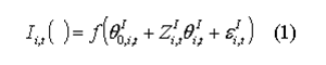
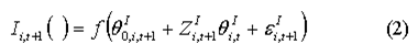
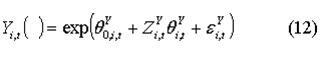
- 2.28
- In dynamic ageing, most of the demographic or labour market variables Zi,tI are themselves endogenous or simulated within the model. Similarly new stochastic terms εi,tI will be generated from the relevant model distributions. Lastly calibration to external factors may be utilised by effectively adjusting the intercept θ0,i,tI to produce
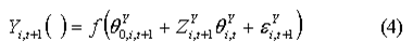
Similarly the level of market income source i can be modelled
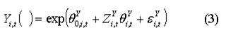
To produce
- 2.29
- In a dynamic microsimulation model which focuses on longitudinal transitions, we can further decompose the error term to account for long term and transitory error components, requiring panel data in the estimation:

- 2.30
- However some models take an intermediate perspective utilising the system to model the main changes in for example an economic downturn, focusing on for example the labour market changes, but making decisions similar to static models by holding the slowly changing variables constant (as for example the education and demographic variables). O'Donoghue et al. (2013) adopted this approach in modelling the impact of the economic downturn in Ireland over a short period. They utilised Labour Force Survey data to calibrate the model in levels. Navicke et al. (2013) applied a simpler alternative in nowcasting the EUROMOD model to the present in order to examine the impact of economic change on poverty. They utilised a set of transition matrices, conditioned on age, gender and education status with data from the EU Labour Force Survey. This essentially involved the application of rates of change in levels, rather than levels as in the case of O'Donoghue et al. (2013).
- 2.31
- We will now consider in practical terms how to apply dynamic ageing. Given the focus in this paper on nowcasting or projecting a cross-section, we will focus solely on cross-sectional dynamic ageing, rather than on longitudinal dynamic ageing (For further information, see O'Donoghue 2010).
- 2.32
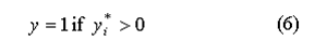
- Models of binary events such as in-work may be modelled using a logit model due to the computational ease of undertaking these simulations. In order to use the estimated probabilities from logistic models within a Monte Carlo simulation, we can draw a set of random numbers such that we predict the actual dependent variable in the base year.
- 2.33
- We define our logit model as follows
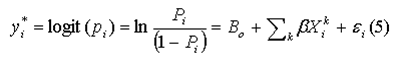
Such that
In order to create the stochastic term, εi, we can use the following relationship:
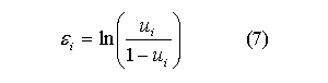
Such that
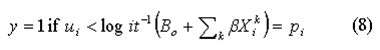
A value of ui that satisfies this is:
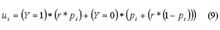
where r is a uniform random number.
- 2.34
- In modelling labour market changes, there is the option of simply modelling in-work status or modelling more deeply changes to the structure of the labour market such as being an employee, self-employed, farmer, etc. In addition changes such as occupation and industry may be required in understanding structural change.
- 2.35
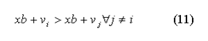
- Multi-category variables such as occupation and industry can be simulated using a multinomial logit model. Multinomial models may be used when the explanatory variables are not choice specific.[1] Disturbance terms for multi-category dependent variables such as occupation or industry are derived from multinomial logit models using the following method. We firstly generate a set of random variables for counter-factual choices using the extreme value distribution:
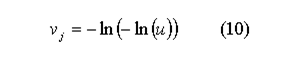
Where u is a uniform random number and j is choice j not the actual choice chosen by the individual in the original data. Our objective now is to choose a random variable from the extreme value distribution, vi for the actual choice i such that:
- 2.36
- Once, we have established the labour force characteristics of each individual, income variables can be modelled using an OLS equation as outlined above
where the disturbance term is normally distributed, recovered directly from the data for those with observed incomes in the data, or generated stochastically for those without a specific income source in the data. The reduced form of these equations means that they can capture labour market changes resulting from changes to the population structure but these are less effective in capturing the impact of external shocks such as the current economic crisis. To incorporate this, we can apply calibration or alignment methods such as in Li and O'Donoghue (2014).
Data
- 3.1
- In order to ascertain the updating, nowcasting and projection methodologies employed by different modelling teams, we undertook a short survey of a sample of modelling teams across the world.
- 3.2
- The survey incorporates a number of components[2]. In the questionnaire, these are divided into different sections numbered as follows:
- Model Characteristics
- Uprating of model using indexation of variables
- Updating of model using reweighting
- Projections of model into the future
- Validation of uprating/updating/projections
- Communicating distributional analysis
- 3.3
- Table 1 provides a summary of the characteristics of the fifteen models in question. Only one of the models (DYNASIM3) can be entirely classified as a dynamic model although the Spanish model and the Irish SMILE model have dynamic components. The majority of the models are updated to the present. The exceptions are the German IZA model, the Hungarian TARSZIM model and the TRIM3 model. The latter model is currently based upon 2010 baseline data and the development of the 2011 baseline data is in progress. We may therefore expect that the non-updating of the model is not a serious limitation for the purposes of simulations and projections. In the case of the German IZA model, the model is frequently used for behavioural analysis and does not involve updating or future projections. The Luxembourg EUROMOD model is the only other model that does not offer future projections.
- 3.4
- We find that modelling teams make projections for many different reasons although poverty estimates appear to be widely practiced. The Australian NATSEM model generates projections for the purposes of welfare program budgeting and reform analysis while the Swedish FASIT model makes projections for estimates of poverty and for some benefits. The Irish SWITCH model makes projections for distributional analysis, poverty impact assessment and measures of work incentives. The UK (Essex) model has recently made projections for policy issues relating to the new Universal Credit. Both the Belgian model and the UK (IFS) model make projections for analysis of poverty and inequality.
- 3.5
- Table 1 shows that there is quite a high variability in the choice of software packages with C++, SAS, STATA being applied by at least two of the models. The DYNASIM3 model relies mainly upon FORTRAN while the IFS relies mostly upon Delphi, the German MIKMOD model utilises Java and the Finnish TUJA model utilises the A programming language.
Table 1: Model Characteristics Country Model Name Static/Dynamic Update the data to the present Future projections Software AUSTRALIA STINMOD Static Yes Yes SAS BELGIUM EUROMOD;Mefisto Static Yes Yes EUROMOD;stat GERMANY IZAΨMOD Static No No Stata GERMANY MIKMOD Static Yes Yes Java HUNGARY TARSZIM Static No Yes MSQL IRELAND SWITCH Static Yes Yes C++ IRELAND Simulation Model of the Irish Local Economy (SMILE) Static, Dynamic and Spatial Yes Yes Stata FINLAND TUJA Static Yes Yes APL (A Programming Language) SPAIN Static/Dynamic Yes Yes SAS/Stata SWEDEN FASIT Static Yes Yes SAS USA Dynamic Simulation of Income Model (DYNASIM3) Dynamic Yes Yes Mainly FORTRAN with a SAS postprocessor USA Transfer Income Model, version 3(TRIM3) Static No but 2010 used 2011 in Progress Yes C++, with other software used for the model's databases and interface UK (IFS) TAXBEN Static Yes Yes Mostly Delphi, with some Stata components UK (Essex) EUROMOD Static Yes Yes C++ Luxembourg EUROMOD Static Yes No C++ & EXCEL
Results
- 4.1
- In this section we report the results of our survey of model builders.
Data Sources for indexation
- 4.2
- In Section 2 of the questionnaire, we requested information on the data sources used to uprate the index values. We also requested information as to whether or not, the relevant index values are provided for different groups.
- 4.3
- For most income variables, the Australian model relies upon average growth rates from external datasets from the Statistics Bureau information. In addition, both Housing values and imputed rents rely upon this source. The model uses the Welfare Agency reports for the updating of benefits and family transfers while the Consumer Index is applied for rent and other housing costs. The average Mortgage payment is aligned with numbers from the statistics bureau as part of the reweighting procedure.
- 4.4
- In the case of the SWITH model in Ireland, index values of weekly salary are applied while benefits are simulated according to the tax-benefit rules. The data sources include the Quarterly Economic Commentary in the case of Employee Earnings and Official forecasts in the case of self-employment income. No updating is applied for mortgage interest and a variety of sources are used to update the asset values of housing and imputed rents. For both the Irish SWITCH model and Australia, the updating of earnings is not disaggregated according to different groups. The Irish SMILE model uses disaggregated occupational and industry specific indices for earnings and GNP per capita for other incomes sources. Projections are undertaken using linear extrapolation for a year.
- 4.5
- In the case of Belgium, the National Bank of Belgium provides the required updating factors for incomes. The Consumer price Index is used for rental income. Benefits are usually simulated but a government website provides index numbers for those variables that are not simulated. Employee earnings are updated based upon separate indices for blue and white collar workers while benefit values are updated separately for Pensions, Minimum income, child benefits, health insurance, education and disability related payments.
- 4.6
- The Swedish model does not update self-employment incomes. The National Institute for economic research provides most of the required data (including mortgage interest) while benefits and family transfers rely upon the rules and calculations in the FASIT model. The IFS uses national statistics to uprate employee, self-employment and farm income. For rental and investment income, the IFS uses the base interest rate to impute capital stock, then uprates the capital stock in line with GDP and uses the current interest rate to impute investment income. The numbers for GDP and the interest rate are due to National Statistics.
- 4.7
- The Luxembourg EUROMOD model uses data from the Ministry of Social Security and the Consumer Price Index to update employee and self-employment income. Mortgage interest is updated using an indexation factor. Some benefits such as the family allowance are not updated in the Luxembourg model.
Reweighting
- 4.8
- In section 3 of the questionnaire, we asked questions about the scale of reweighting being undertaken within each model. The results are presented below in table 2.
Table 2: Reweighting Country Model Name Adjust Survey Weights Reweighting methods Time taken to do this Task AUSTRALIA STINMOD Yes GREGWT BELGIUM EUROMOD;Mefisto No GERMANY IZAΨMOD No GERMANY MIKMOD Yes Newton-Raphson 15 -20 person days HUNGARY TARSZIM No IRELAND SWITCH Yes CALMAR 10 Days IRELAND SMILE Yes Reweight2 2 Days FINLAND TUJA Yes CLAN97 One Day (6 times a Year) SPAIN No SWEDEN FASIT Yes CLAN97 3 Days USA (DYNASIM) Dynamic Simulation of Income Model (DYNASIM3) No USA (TRIM3) Transfer Income Model, version 3(TRIM3) No UK (IFS) TAXBEN Yes Reweight2 One Day UK (Essex) EUROMOD No Luxembourg EUROMOD No - 4.9
- The above results show that 7 of the 15 models allow for the adjustment of survey weights; Australia, Ireland (SWITCH AND SMILE), Finland, Sweden, the German MIKMOD model, and the UK IFS model. These models rely upon some different reweighting methods. These include GREGWT, Newton-Raphson, CALMAR, CLAN and Reweight2. There is some variability in the time taken to do this task across countries. The Irish SWITCH model requires the input of ten person days while the Swedish FASIT model requires three days and the IFS model only one day. Some of this variance can be attributed to differences in the frequency of reweighting. For instance, the reweighting of the Finnish CLAN97 model usually requires just one person day but this process is usually repeated six times per year. This is the model used by Immervoll et al. (2005) as discussed in section 2 and was developed by Statistics Sweden (Lundström and Särndal 2001).
Future Projections
- 4.10
- In this section, we summarise the responses in relation to the use of projections. The results indicate that 10 of the 15 models apply future projections. All of these models update price and income indices. The Dynasim3 model, the Spanish model and the UK (Essex) model are the only models that do not adjust in some way for population weights. For the future projections, the Belgian EUROMOD model does not adjust for tax-benefit rules. None of the fifteen models are linked to a macro-economic model although the IFS have used the macro forecasts of others as an input to reweighting and uprating processes. The DYNASIM3 model has used macro models for select analyses but this is not routine. In terms of the time span of projections, there are some variations. The Irish SWITCH and SMILE models projects one year forward to identify the impact of tax-benefit policy changes. Both the Swedish FASIT model and the Finnish TUJA model are projected forward to 2016 and the IFS model is projected forward for each year until 2015 and also projected for 2020. The Australian STINMOD is projected five to ten years into the future. The Belgian EUROMOD and the DYNASIM3 model are projected for a much more distant time into the future. It appears that models focused on a particularly long time horizon are less likely to apply adjustments for tax-benefit rules.
Table 3: Future Projections Country Model Name Future Projection To What Time Update price and income indices? Adjust population weights? Adjust tax-benefit rules? Link to macro-economic model? Dynamic Ageing AUSTRALIA STINMOD Yes 5-10 years Yes Yes Yes No No BELGIUM EUROMOD;Mefisto Yes 50 years Yes Yes No No Not yet[3] GERMANY IZAΨMOD No GERMANY MIKMOD Yes 2017 Yes Yes Yes No No Hungary TARSZIM No Ireland SWITCH Yes 1 Year Yes Yes Yes No No Ireland SMILE Yes 1 Year Yes Sometimes Yes No Yes FINLAND TUJA Yes 2016 Yes Yes Yes No No SPAIN Yes 2015 Yes No Yes No Sometimes SWEDEN FASIT Yes 2016 Yes Yes Yes No No USA Dynamic Simulation of Income Model (DYNASIM3) Yes 2087 (75 years) Yes No Sometimes No Yes USA Transfer Income Model, version 3(TRIM3) No UK (IFS) TAXBEN Yes Each year to 2015, and 2020 Yes Yes Yes No Partial UK (Essex) EUROMOD Yes Ad Hoc Purposes Yes No Yes No No Luxembourg EUROMOD No Time Taken
- 4.11
- In table 2, we reported the time normally taken by each team to reweight the microsimulation model. In table 4, we report the time taken for all four different components of updating a dataset or model:
- Indexation
- Reweighting
- Updating
- Projections
- 4.12
- There is significant time variability in relation to the different components with in each case the standard deviation across models about the same or higher than the mean. This reflects differences in
- Complexity
- Resources
- Experience
- Development Stage
- 4.13
- The results identified apply to models for individual countries, although a number of users utilise the EUROMOD framework. It may be possible to achieve economies of scale in the move to a multi-country analysis. It should also be noted that the sample of models within our survey was not a random sample, but rather a subset of the more experienced modelling teams. There are likely to be learning costs with less experienced teams.
- 4.14
- In addition, we find some variability in the amount of information that is available online for each model. Some model websites are very detailed such as the website for the Belgian MEFISTO EUROMOD model. This includes links to papers and permits registered online users to simulate the effects of hypothetical reforms using two simplified versions of the model i.e. the MEFISTO Light and MEFISTO Basic. Examples of hypothetical reforms include a reform of the personal income tax or the VAT-system. The Australian NATSEM model website gives links to a large number of publications as does the website for the Irish ESRI SWITCH model which also provides a very thorough overview of recent research findings. The website for the IZA model supplies a long list of publications and outlines the simulation steps within the model. Information about the Irish SMILE model can be found through the search engine of the TEAGASC rural economy and development website including papers and reports. A wide range of publications and presentations for the Finnish TUJA model can be found from the VATT website using the search engine. DeCoster et al. (2008) provide a comparison of the TUJA model with other microsimulation models. The Statistics Sweden website provides a good deal of information about the FASIT model in both the Swedish and English language which can be found through the websites search engine. The website of the Urban Institute provides a detailed a primer on the DYNASIM3 model by (Favreault & Smith 2004) as well as a large number of publications for both the TRIM3 and DYNASIM3 models. The IFS website provides a number of publications relating to the TAXBEN model including a useful overview by Brewer (2009).
Table 4: Days of Work Time for Nowcasting Components Country Organisation Model Webpage Index Reweight Update Project AUSTRALIA NATSEM STINMOD http://www.natsem.canberra.edu.au/models/stinmod/ 20 Varies Days to Weeks Varies Days to Weeks BELGIUM KU Leuven EUROMOD; Mefisto http://www.flemosi.be/easycms/home 5 25 90 GERMANY IZA IZAΨMOD http://www.iza.org/en/webcontent/politics/izapsimod 3 GERMANY Fraunhover MIKMOD http://publica.fraunhofer.de/documents/N-234224.html 15 18 HUNGARY TÁRKI Social Research Institute TARSZIM 27.5 35 IRELAND ESRI SWITCH https://www.esri.ie/research/research_areas/taxation_welfare_and_pensions/ 10 10 20 20 IRELAND TEAGASC SMILE http://www.agresearch.teagasc.ie/rerc/ 5 2 10 20 FINLAND Government Institute for Economic Research (VATT) TUJA http://www.vatt.fi/en/ 11 1 4 SPAIN 10 21 10 SWEDEN Statistics Sweden FASIT http://www.scb.se/en_/ 30 3 5 10 USA (DYNASIM) The Urban Institute Dynamic Simulation of Income Model (DYNASIM3) http://www.urban.org/index.cfm 8 USA (TRIM3) The Urban Institute Transfer Income Model, version 3(TRIM3) http://www.urban.org/center/ibp/index.cfm 65 UK (IFS) IFS TAXBEN http://www.ifs.org.uk/ 0.5 1 5 8 UK (Essex) ISER EUROMOD https://www.iser.essex.ac.uk/euromod 1.5 10 12 Luxembourg CEPS/INSTEAD EUROMOD http://www.ceps.lu/ 3 5 Average 10.8 10.0 15.1 24.3 Range 29.5 34.0 62.0 82.0 StDev 9.9 12.7 17.4 29.4
Conclusions
- 5.1
- In this paper, we describe the various components that can be included in the nowcasting of a Microsimulation model. We undertake a survey of a number of modelling teams globally to investigate for each component the variability in the current practices. Modelling teams are selected based on their experience and breadth of use in the methodologies of nowcasting. The nowcasting methodologies include indexation to adjust for wage growth, the updating for changes in tax-benefit policy, the use of ageing techniques to account for changes to the population and labour market structure and the use of projections. We find that many of the modelling teams incorporate all or most of these methodologies in adjusting for changes to the income distribution over time.
- 5.2
- Modelling teams are increasingly utilising variants of these methods for projections, most of which are relatively short-term. Poverty analysis appears to be a motivation for many of these projections but inequality analysis and work incentives also appear quite popular. It appears that the ultimate goals of the various modelling teams are an important determinant of nowcasting practices. For instance, the German IZA model is frequently targeted towards behavioural analysis rather than projections so that data reweighting and income uprating are excluded. There is growing interest within the Microsimulation literature in methodologies that can be used to adjust the survey weights to account for recent economic changes such as unemployment and labour force participation. We find that approximately half of the modelling teams make such adjustments so there is perhaps scope for further adoption of reweighting methods.
- 5.3
- There appears to be significant variability between modelling teams in the time taken to nowcast a model, which could perhaps be reduced through multi-country analysis. We find that there is a good deal of information available online with respect to the work of these modelling teams with the Belgian team appearing to be particularly advanced in providing registered online users with the opportunity to simulate hypothetical reforms of the Belgian tax-benefit system. These initiatives are not however, always feasible for other modelling teams and there are likely to be learning costs associated with being a less experienced team which limits the number of components that can be modelled reliably. The comparative analysis outlined in this paper could be a useful guide for modelling teams wishing to learn from one another so that a wider number of modelling teams will eventually find the capacity to reliably adopt new components to their Microsimulation models.
Acknowledgements
- This work has been carried out within the framework of a service contract defined and financed by and whose results belong to the European Commission – Eurostat.
Notes
-
1There is a large literature on using choice specific models for modelling multi-category choices as in the case of structural labour supply equations (see Van Soest 1995; Callan et al. 2007). However we use a calibration mechanism described below which dominates the behavioural operation of these models.
2It should be noted that the survey also collected information in relation to changes in the tax-benefit system. However, we do not discuss that in this paper.
3in process with model MIDAS of Federal Planning Bureau Belgium
References
-
ABELLO A., Brown L., Walker A. &Thurecht L. (2003). An Economic Forecasting Microsimulation Model of the Australian Pharmaceutical Benefits Scheme. Technical Paper no. 30. Canberra: The National Centre for Social and Economic Modelling.
ADELZADEH, A. (2001). NIEP Social Policy Model: policy tool for fighting poverty in South Africa. National Institute for Economic Policy.
ATKINSON, A. B., Rainwater, L., & Smeeding, T. M. (1995). Income distribution in OECD countries: evidence from the Luxembourg Income Study. Paris: Organisation for Economic Co-operation and Development.
BOURGUIGNON, F., Fournier M & Gurgand, M. (2001). Fast Development with a Stable Income Distribution: Taiwan, 1979-94. Review of Income and Wealth, 47(2), 139–163. [doi:10.1111/1475-4991.00009]
BOURGUIGNON, F., Ferreira, F.H.G., & Leite, P.G. (2002). Beyond Oaxaca-Blinder : Accounting for Differences in Household Income Distributions Across Countries. DELTA Working Paper 2002-04. [doi:10.1596/1813-9450-2828]
BREWER M. (2009). TAXBEN: the IFS static tax and benefit micro-simulation model presented at a seminar called 'UK Microsimulation: Bridging the Gaps', at the BSPS Conference, University of Sussex, September 2009.
BREWER M., Dickerson A., Gambin L., Green A., Joyce R., & Wilson R. (2012). Poverty and Inequality in 2020 Impact of Changes in the structure of Employment. York: Joseph Rowntree Foundation
CALLAN T.,Van Soest A. & Walsh, J. R. (2007). Tax Structure and Female Labour Market Participation: Evidence from Ireland, WP208, Economic and Social Research Institute (ESRI).
CALLAN, T., Keane C., Walsh J. R., & Lane, M. (2010). From Data to Policy Analysis: Tax-Benefit Modelling using SILC 2008. Journal of the Statistical and Social Inquiry Society of Ireland Vol. XL
CREEDY, J. (2003). Survey Reweighting for Tax Microsimulation Modelling. Treasury Working Paper Series 03/17.
DECOSTER, A., De Swerdt, K., Orsini, K., Lefèbvre, M., Maréchal, C., Paszukiewicz, A., Perelman, S., Rombaut, K., Verbist, G. and Van Camp, G. (2008). Valorisation of the microsimulation model for social security MIMOSIS. Final report project AG/01/116. Leuven
DEVILLE, J.C. & Särndal C.E. (1992). Calibration estimation in survey sampling, Journal of the American Statistical Association, 87(418), 375–382. [doi:10.1080/01621459.1992.10475217]
FAVREAULT, M. & Smith, K. (2004) 'A Primer on the Dynamic Simulation of Income Model (DYNASIM3)', The Retirement Project, Urban Institute, Washington.
FLORY J. & Stöwhase, S. (2012). MIKMOD-ESt: A Static Microsimulation Model of Personal Income Taxation in Germany, International Journal of Microsimulation, Interational Microsimulation Association, 5(2), 66–73.
HANCOCK, R., Hills J., Zantomio F., & Sutherland, H. (2008). Keeping up or falling behind? The impact of benefit and tax uprating on incomes and poverty ISER Working Paper Series No. 2008-18. University of Essex: Institute for Social and Economic Research
IMMERVOLL, H. (2000). Fiscal Drag - An Automatic Stabiliser? , Cambridge Working Papers in Economics 0025, Faculty of Economics, University of Cambridge.
IMMERVOLL, H., Lindström, K., Mustonen, E., Riihelä, M., & Viitamäki, H. (2005). Static data ageing techniques. Accounting for population changes in tax-benefit microsimulation. EUROMOD Working Paper, EM7/05.
JENKINS S. & Van Kerm P. (2014). The Relationship Between EU Indicators of Persistent and Current Poverty, Social Indicators Research, Springer, vol. 116(2)
KLEVMARKEN, N. A. (1997). Modelling Behavioural Response in EUROMOD, Cambridge Working Papers in Economics 9720, Faculty of Economics, University of Cambridge.
LE GUENNEC, J. & Sautory, O. (2003). La macro Calmar2, manuel d'utilisation, document interne INSEE.
LI, J., & O'Donoghue, C. (2014). Evaluating binary alignment methods in microsimulation models. Journal of Artificial Societies and Social Simulations 17 (1), 15 https://www.jasss.org/17/1/15.html.
LUNDSTRÖM, S., & Särndal, C.E. (2001). Estimation in the Presence of Nonresponse and Frame Imperfections. Stockholm: Statistics Sweden.
NAVICKE, J., Rastrigina O. & Sutherland, H. (2013). Nowcasting Indicators of Poverty Risk in the European Union: A Microsimulation Approach, Paper presented to EU-SILC Conference, Vienna.
O'DONOGHUE C. (2001a). Dynamic Microsimulation: A Survey, Brazilian Electronic Journal of Economics. Department of Economics, Universidade Federal de Pernambuco, 4(2).
O'DONOGHUE C., (2001b). Redistribution over the Lifetime in the Irish Tax-Benefit System: An Application of a Prototype Dynamic Microsimulation Model for Ireland, Economic and Social Review, 32(3), 191-216.
O'DONOGHUE, C., Hynes S. and Lennon, J. (2009). The Life-Cycle Income Analysis Model (LIAM): A Study of a Flexible Dynamic Microsimulation Modelling Computing Framework, International Journal of Microsimulation, 2(1) 16-31.
O'DONOGHUE, C. (2010). Life-Cycle Income Analysis Modelling, Lambert Academic Publishing AG & CO.KG
O'DONOGHUE C., Sutherland H. & Utili, F. (2000). Integrating Output in EUROMOD: An Assessment of the Sensitivity of Multi-Country Microsimulation Results, in Mitton L., H. Sutherland & M. Weeks (eds.), Microsimulation in the New Millennium. Cambridge: Cambridge University Press.
O'DONOGHUE C., Loughrey J. & Morrissey, K. (2013). Using the EU-SILC to model the impact of the economic crisis on inequality, IZA Journal of European Labor Studies, 2(1), 1–26 [doi:10.1186/2193-9012-2-23]
OTA, R. & Stott, H. P. (2007). A New New Zealand Static Microsimulation Model - Challenges With Data. Paper presented to the International Microsimulation Association, Vienna, July.
PUDNEY S.E. (1992). Dynamic Simulation of Pensioner's incomes: methodological issues and a model design for Great Britain., Dept. of Applied Economics Discussion paper no MSPMU 9201, University of Cambridge.
REDMOND, G., Sutherland, H., & Wilson, M. (1998). The arithmetic of tax and social security reform: a user's guide to microsimulation methods and analysis (Vol. 64). Cambridge University Press.
SUTHERLAND H. (ed.) (2001). EUROMOD: an integrated European Benefit-tax model, Final Report, EUROMOD Working Paper EM9/01, Microsimulation Unit, Department of Applied Economics, University of Cambridge
VAN SOEST, A. (1995). Structural models of family labor supply: a discrete choice approach, Journal of Human Resources, 30(1), 63–88. [doi:10.2307/146191]