
 Abstract
- Behavioural economics highlights the role of social preferences in economic decisions. Further, populations are heterogeneous, suggesting that the composition of social preference types within a group may impact the ability to sustain voluntary public goods contributions. We conduct agent-based simulations of contributions in a public goods game, varying group composition and the weight individuals place on their beliefs versus their underlying social preference type. We then examine the effect of each of these factors on contributions. We find that social preference heterogeneity negatively impacts provision over a wide range of the parameter space, even controlling for the share of types in a group.
- Keywords:
- Social Preferences, Group Composition, Beliefs, Agent-Based Simulation
Introduction
- 1.1
- Adequate public goods provision is an important determinant of social welfare, especially the welfare of the poor (Besley & Ghatak 2006; Fan et al. 1999; Fan et al. 2002; Squire 1993; World Bank 1990). Examples of these welfare-enhancing public goods include health services (e.g. Besley & Ghatak 2006; Chen et al. 1999), schools (e.g. Alesina et al. 1999; Besley & Ghatak 2006; Labaree 1997), clean water (and the supporting infrastructure required, e.g. Besley & Ghatak 2006; Shafik 1994), urban sanitation (e.g. Alesina et al. 1999; Shafik 1994) and roads (e.g. Alesina et al. 1999; Besley & Ghatak 2006). Ensuring an adequate level of these and other public goods, through either government or voluntary provision, is important for the overall well-being of the citizenry.
- 1.2
- Traditional economic analysis suggests private under-provision of these vital goods (Hardin 1968; Olson 1965). Under-provision of voluntarily provided public goods stems from individuals selfishly considering only their own costs and benefits associated with providing the good without regard for the benefits accrued to others (Cornes & Sandler 1996). Central to this conclusion is the hypothesis that all individuals are selfish. Insights from behavioural and experimental economics suggest that, while individuals often make choices in keeping with their own self-interest, many individuals are willing to sacrifice their own well-being in order to improve the lot of others (for a recent review see Gächter 2007). Incorporating the welfare of others into one's own utility function is referred to as social preferences: Significant heterogeneity in the types of social preferences held by members of society has been robustly documented (see e.g. de Oliveira et al. 2013; Fischbacher et al. 2001; Fischbacher & Gächter 2010 among others).
- 1.3
- With this social preference heterogeneity in a society, the composition of social preferences within groups may also impact provision (e.g. de Oliveira et al. 2013; Fischbacher & Gächter 2010; Gächter and Thöni 2005). We build upon the results of Fischbacher and Gächter (2010), conducting an agent-based simulation. Agent-based simulations are particularly useful in this area since the composition of populations cannot be exogenously varied and simulations runs can be systematically analysed.
- 1.4
- Previous research has well-documented a negative relationship between group heterogeneity and public goods provision in a variety of publicly- and privately-provided public goods (e.g. Alesina et al. 1999; Miguel & Gugerty 2005; Vigdor 2004). This heterogeneity can take many forms, including but not limited to race or ethnicity (e.g. Alesina et al. 1999), language (e.g. Easterly & Levine 1997), and age (Poterba 1997). We complement the existing literature by examining social preference heterogeneity.
- 1.5
- Specifically we conduct an agent-based simulation where we vary the social preference composition of the group. We examine voluntary public goods provision in these groups under several rules for determining contributions. We then examine the role of group composition in provision, paying particular attention to the impact of social preference heterogeneity. Note that while we are using the standard fractionalization index we are considering a new type of diversity not typically discussed in the literature: the diversity of social preferences. We then examine the robustness of our results to a variety of parameter specifications.
- 1.6
- We find that social preference heterogeneity negatively impacts the level of voluntary contributions in some settings but not in others.[1] When we restrict the analysis to the most common social preference types, a robust negative relationship exists. For the full set of social preference types, a significantly negative relationship only exists for a small portion of the parameter space. These results complement and extend the prior literature, which has examined fractionalization based on observable characteristics. Our agent-based approach allows for a flexible and complete testing of behaviour heterogeneity in groups. We now turn to a discussion of previous research before detailing our agent-based simulation and the results from our experiment.
Previous Research
- 2.1
- The willingness of individuals to work together for the common good can be impacted by many factors. While we focus on social preference heterogeneity, our study intersects several existing lines of research. We will now discuss them in turn.
Diversity, Public Goods, and Welfare
- 2.2
- Perhaps the most direct established link between heterogeneity and welfare is a well-documented negative relationship between ethnic diversity and growth, though there is some debate as to whether the mechanism is causal (Alesina et al. 2003; Easterly & Levine 1997). Rising incomes directly improve welfare, but this is not the only mechanism through which ethnic diversity may impact welfare. Importantly, racial fractionalization has been suggested to be negatively related with infrastructure development (Alesina et al. 2003), which may hamper both current and future well-being. Additionally, ethnic fractionalization is correlated with governance quality (Alesina et al. 2003; Mauro 1995). As populations become more ethnically diverse these effects may be exacerbated.
- 2.3
- Fractionalization, also referred to as heterogeneity or diversity, has been shown to negatively impact the provision of public goods. The negative relationship holds for a broad spectrum of goods, including: goods provided by the government (e.g. Alesina et al. 1999; Banerjee & Somanathan 2007), goods that are voluntarily provided (e.g. Miguel & Gugerty 2005; Vigdor 2004), and for participation in the community (e.g. Alesina and La Ferrara 2000; Costa & Kahn 2003). It is important to note that heterogeneity may occur along many dimensions, including race or ethnicity as well as language (e.g. Alesina et al. 1999; Costa & Kahn 2003; Easterly & Levine 1997), income (e.g. Costa & Kahn 2003), and birthplace (e.g. Costa & Kahn 2003).
- 2.4
- While the negative relationship between fractionalization and public good provision is well documented, appropriate social policies can help overcome these divisions (e.g. Banerjee & Somanathan 2007; Miguel 2004). Doing so will help increase the well-being of the poor, as documented through the link between public goods provision and welfare (e.g. Besley & Ghatak 2006; Fan et al. 1999; Fan et al. 2002; Squire 1993; World Bank 1990). Further, since diversity could theoretically be positively related to growth by spurring new ideas and innovation, if the negative spiral can be broken, then the positive effects may dominate. One way to break the spiral may be through appropriately designed institutions (Easterly 2001).
- 2.5
- Due to the absence of data, previous studies have not investigated the possible relationship between social preference heterogeneity and voluntary provision, which we do. We find that the negative impact of fractionalization extends to this domain. We now turn to a discussion of the literature on social preference and group composition.
Social Preferences, Group Composition, and Public Goods
- 2.6
- These studies point to the negative effects that social diversity can have in economies in general (Alesina et al. 2003; Easterly & Levine 1997; Mauro 1995) and on public goods provision in particular (Alesina et al. 1999; Miguel & Gugerty 2005; Vigdor 2004). One common approach is to rely on demographics like ethnicity to examine heterogeneity and then argue that this heterogeneity impairs the ability of social preferences--like trust or conditional cooperation--to function. This is due, at least in part, to the inability to either measure or vary social preference diversity on a large scale. Studies that have examined social preferences in this setting, via survey measures, have found higher self-reported levels of trust related to growth (Zak & Knack 2001).
- 2.7
- The control available through experimentation has robustly determined that individuals are willing to sacrifice their self-interest in order to help others (Camerer & Fehr 2004; Charness & Rabin 2002; Fehr & Fischbacher 2002; Henrich et al. 2001; Roth et al. 1991). Further, a set of distinct social preference types and been identified and measured experimentally (Ahn et al. 2003; Burlando & Guala 2005; de Oliveira et al. 2013; Fischbacher & Gächter 2010; Fischbacher et al. 2001; Herrmann and Thöni 2009; Kurzban & Houser 2005).
- 2.8
- In addition to the traditional Nash (or selfish) type of individual, several common social preference types have been identified. Conditional Cooperators, or reciprocators, make up the largest proportion of the population and are individuals who will give more when they believe others will give (Burlando & Guala 2005; Croson 2007; de Oliveira et al. 2013; Frey & Meier 2004; Fehr & Gächter 2000; Fischbacher & Gächter 2010; Fischbacher et al. 2001; Kurzban & Houser 2005). In fact, a strict (or perfect) conditional cooperator will give exactly what he expects others to contribute. Unconditional Cooperators, also referred to simply as cooperators, are individuals who give a set amount no matter what others give (Burlando & Guala 2005; Kurzban & Houser 2005).[2] Economic Altruists want the public good to be provided but prefer for someone else to provide it,[3] which results in own contributions decreasing in the contributions of others (Croson 2007). Threshold players are individuals who refuse to contribute until others are giving what they deem as 'enough' and then contribute fully. Finally, Hump, also referred to as triangle, players are individuals who behave like a conditional cooperator when group members are contributing low amounts and behave like a pure altruist when group members are contributing high amounts (Fischbacher & Gächter 2010; Fischbacher et al. 2001; Herrmann & Thöni 2009).
- 2.9
- Papers that focus on identifying types generally report results of the free-riders, conditional cooperators, and hump and then lump all other types into an 'other' category (e.g. Fischbacher et al. 2001; Herrmann & Thöni 2009). We allow all types in the estimation in the interest of completeness. Further details about the preference types and their implementation in the simulation are discussed in section 3.
- 2.10
- Social welfare in public goods games, measured as the total earnings of subjects or as contributions as a percentage of the social optimum, are higher in groups with more conditional cooperators in them (e.g. de Oliveira et al. 2013; Kurzban & Houser 2005). While a more thorough study is warranted, since some of the social preference types comprise only a small portion of the population, it would be difficult to systematically varying all types using human subjects in a laboratory. We therefore conduct an agent-based simulation to examine the issue.
Agent-Based Simulation
- 3.1
- An agent-based model has been developed to simulate the contributions of individuals to a public good. We use the structure of the public goods game, which has been studied widely experimentally (see Chaudhuri 2011; Ledyard 1995 for reviews). In the typical public goods game, agents receive an endowment which they can allocate between an individual account and a group account. Tokens deposited in the individual account are kept by the agent while contributions sent to the group account are multiplied by some factor and divided evenly between all agents.[4] So long as the factor is strictly greater than one and strictly less than the group size this game results in a distinct Nash equilibrium (i.e. participants decide to keep everything) and a distinct social optimal (i.e. participants decide to contribute all tokens to the group account).
- 3.2
- The literature is unclear as to whether social preference types arise from corresponding utility functions or whether they are only strategies. The process through which utility functions and interact to produce actions is an important avenue for future behavioural research. For purposes of our simulation, agents are programmed as adhering to a strategy, with a different strategy for each social preference type. For purposes of the simulation, we will refer to these as the agents' 'contribution preferences' or 'social preference types.'
- 3.3
- With multiple social preference types, behaviour may be determined by their contribution preferences and their beliefs, rather than only payoff-maximization. We are able to separate payoff-maximization in this manner because the payoff-maximizing strategy is always the same in the game with finite rounds: to contribute zero.
- 3.4
- For the purpose of the simulation, when we refer to an agents' programmed strategy, we consider three scenarios. Specifically, the action chosen in a particular period can be a) completely determined by preference type, b) completely determined by beliefs or c) determined by a combination of type and beliefs. The agent's programmed strategy is then executed over ten rounds with the same group members. Specifically, agent i calculates her contribution to the public good Ci,t at time t using the following equation:
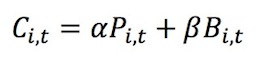
(1) where Pi,t is agent i's underlying preference at period t and Bi,t is agent i's subjective belief at period t. Agent i's preference Pi,t may further be a function of her beliefs Bi,t (see eq. 3 below), depending on preference type. Hence, agent i's contribution is a weighted average of her preferences and beliefs, where the weights α,β are set by the model.
- 3.5
- To begin, we estimate four models which vary the programmed strategy employed by the agents. These include one based solely on the agents' preferences and three which weight preferences and beliefs using the estimation results from Fischbacher and Gächter (2010, we use their model names below). Specifically, these are:
- Fully Preference Driven: where α = 1 and β = 0;
- Belief Model 3 (α = 0.242 and β = 0.666);
- Belief Model 4a (α = 0.443 and β = 0.545); and
- Mixed Belief Model 4b-c (where α = 0.385 and β = 0.582 for the first 5 rounds, and α = 0.614 and β = 0.376 for the last 5 rounds).
- 3.6
- Results in Section 5 will be based upon these models, and we will discuss the robustness of the results to alternate parameter specifications in Section 6.
- 3.7
- For all types of players, agent beliefs are determined in the first period through a random draw between zero and the maximum possible contribution. After the initial round, beliefs are computed using the following formula:
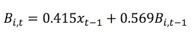
(2) Thus, Bi,t is simply the weighted average of others' contributions at period t-1, xt–1 and agent i's own beliefs in period t-1, Bi,t–1. These weights on others' contributions and own beliefs follow Beliefs Model 3 in Fischbacher and Gächter (2010). Since we focus on the role of group composition, rather than information about the composition, we do not allow the first-round beliefs to vary by group composition.[5]
- 3.8
- The general formulation of agent i's underlying preference is given by the following:
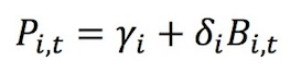
(3) where γi and δi are agent i's preference parameters, which are stable over periods and constant for all individuals of the same preference type. Preference types can be broadly classified as either unconditional or conditional. Within each of these are further distinctions leading to a total of 9 different preference types:
- 3.9
- Unconditional: These agents have underlying preferences that are independent of their beliefs about the amount contributed by other group members, that is δi = 0 (see e.g. Burlando & Guala 2005; de Oliveira et al. 2013; Fischbacher & Gächter 2010; Fischbacher et al. 2001; Herrmann & Thöni 2009; Kurzban & Houser 2005). Within this broad categorization, we have five distinct types of contribution preferences:
- Free Riders (γi =0, δi = 0): The contribution preference is set to zero for all periods, which corresponds to the Nash equilibrium level of contributions in the finitely-repeated linear VCM regardless of the other types in the group (e.g. Burlando & Guala 2005; de Oliveira et al. 2013; Fischbacher & Gächter 2010; Fischbacher et al. 2001; Herrmann & Thöni 2009).
- Low Cooperators (γi= [1,9], δi = 0): The contribution preference in the first period is set by a random draw from a uniform distribution within the lower half of the contribution range, excluding the lowest value (and is thus distinct from the Free Rider type). Once drawn, this value is constant for all periods.
- High Cooperators (γi= [10,19], δi = 0): The contribution preference in the first period is set by a random draw from a uniform distribution within the upper half of the contribution range, excluding the top value. Once drawn, this value is constant for all periods.
- Maximum Cooperators (γi= 20, δi = 0): The contribution preference in the first period is set to the maximum possible contribution for every simulated period.
- Noisy Players (γi = εi,t ∈ [0,20], δi = 0): Some individuals do not have well-defined preferences in this environment, while others may be confused or make decisions with errors. To allow for this possibility, we include a player whose contribution preference is 'noisy' (Burlando & Guala 2005; Fischbacher et al. 2001). In every round, the contribution preference is calculated by a random draw from a uniform distribution within the full range of possible contributions.
- 3.10
- Conditional: These social preference types have underlying preferences that are conditional on their beliefs about the amount that group members will contribute (i.e. δi = 0):Burlando & Guala 2005; de Oliveira et al. 2013; Fischbacher & Gächter 2010;Fischbacher et al. 2001; Herrmann & Thöni 2009; Croson 2007). Within this broad categorization, we have four distinct types of contribution preferences:
- Conditional Cooperators (γi = 0, δi = 1): This type of agent has a preference for contributing the amount according to the belief regarding how other group members will contribute in a given period t (e.g. Burlando & Guala 2005; de Oliveira et al. 2013; Fischbacher and Gächter 2010; Fischbacher et al. 2001; Herrmann & Thöni 2009).
- Economic Altruists (γi = 20, δi = −1): Under the economic definition of pure altruism, the welfare of others enters one's own utility function as a public good. The implication is thus that individuals want others to be cared for, but own-provision and other-provision are substitutes. Thus, as other group members give more to the public good the pure altruist will actually give less: The giving of others crowds out own-giving (as set out in Croson 2007; see also Andreoni 1989, 1990 as well as Becker 1974).This means that they prefer to contribute less as their beliefs about other group members increase.
- Threshold Players (γi = 0 if Bi,t < 10, δi = 0) and (γi = 20 if Bi,t ≥ 10, δi = 0): Individuals with this social preference type prefer not to contribute when they believe other group members are giving less than their threshold amount and prefer to contribute fully when their beliefs about their group members are above their threshold amount. The threshold level has been set to half the maximum possible contribution for all agents.
- Hump (Triangle) Players (γi = 0, δi = 1 if Bi,t < 10) and (γi = 20, δi = -1 if Bi,t ≥ 10): Individuals with this contribution preference prefer to behave like conditional cooperators for low levels of beliefs about others giving, and like economic altruists for high levels of beliefs about others giving (Fischbacher & Gächter 2010; Fischbacher et al. 2001; Herrmann & Thöni 2009). Similar to threshold players, the threshold level has been set to half the maximum possible contribution for all agents.
- 3.11
- Note that for the models where beliefs are absent (β = 0, as in the Fully Preference Driven model), actual contributions of others at period t−1, xt−1 are used to calculate contribution preferences (in eq. 3 above) for all conditional types.
- 3.12
- The overall group composition is defined by how many agents with each contribution preference are in the group. Groups can be created with an arbitrary number of participants and each participant will have a stable social preference type associated throughout the simulation runs. The simulation model is initialized by setting the group size to four, the maximum possible contribution to 20 and then set α and β for the run.
- 3.13
- Every individual agent is created with a contribution preference type and, if set, also a belief model. Each simulation run is asynchronous (i.e. agent types are processed without a fixed order to avoid computational path dependency). Each simulated period will compute the following:
- If beliefs are included, a random initial belief value, Bi1, (ranging from zero to the maximum possible contribution) for every type of agent in the simulated public goods group.
- Unconditional Low and High cooperators randomly generate a contribution preference value, Pi, within the lower and upper half of the contribution range, respectively.
- Noisy cooperators randomly generate a contribution preference value, Pit, within the contribution space.
- Every type of agent computes Cit based on equation 1.
- If beliefs are included, every individual agent updates beliefs based on equation 2.
- If the final period has been reached, halt the simulation, otherwise repeat from step 3.
- 3.14
- The pseudo-random values included in the simulation model were implemented using the Mersenne Twister method (Matsumoto & Nishimura 1998) to compute uniform distributions. These include the aforementioned initial random setting of values for certain agent types and a new value for each period for the noisy agent. Due to these non-deterministic features, the model is not fully driven by the initial conditions. Further, notice that, with the exception of the noisy agent, Pit, Bit and Cit are not calculated with errors. Instead of completely eliminating noise from the simulation, the noisy player has been included due to prior observation (Burlando & Guala 2005; Fischbacher et al. 2001). Specifically, we include the noisy player as one of the possible contribution preference type, not to add noise to the data. We thus test their role along with the other possible social preference types found in the public goods game setting.
- 3.15
- The simulation model allows to systematically analyse every group composition, with regards to contribution preference type. Finally, the model allows changes in the relative weights of beliefs and preferences as they contribute to contribution decisions. The advantage of using the agent-based approach to this research problem is to fully account for the heterogeneous interaction occurring at the individual level, which ultimately leads to insights at the group level. The model has been implemented in NetLogo 3.15 and the experiments ran on Oracle's Java 7 on a 64 bit Linux kernel server with 32 GB of memory, generating a text file of 9.7 gigabytes. Should the reader wish to read the simulation source, please contact the corresponding author.
Description of Data
- 4.1
- Data are generated using the agent-based simulation described in the preceding section. The dependent variable in the analysis is the average number of tokens contributed to the group account in period t, ranging from 0 (the Nash equilibrium in the traditional game) to 20 (the social optimum).
- 4.2
- As previously described, we use groups of four agents, which parallels both the experimental and simulation results in Fischbacher and Gächter (2010). Groups are allowed to vary between completely homogeneous and completely heterogeneous, with all possible combinations in between, making use of all nine contribution preference types. This results in 495 distinct group compositions. For each group composition the simulation runs 100 separate times with 10 rounds for each run. This results in a data set of 49,500 groups and 495,000 data points for the Fully Preference Driven and Belief Model 3 models.
- 4.3
- In accordance with Fischbacher and Gächter (2010), the data for Belief Model 4a and Mixed Belief Model 4b-c are restricted to three agent types (Free Riders, Conditional Cooperators, and Hump Players), yielding 15 distinct group combinations. With 10 rounds executed a 100 independent times, this process generates a sample of 15,000 data points. Fischbacher and Gächter (2010) note that every other type is excluded in their models because these (approximately 10% of their sample) are denoted as "confused subjects" meaning that they were unable to classify these agent types. Since we utilize their parameters, we restrict our sample as well.
Results: Social Preference Heterogeneity
- 5.1
- We now turn to our analysis of the social welfare achieved in each of these simulated groups. Recall that the unit of observation is the average number of tokens contributed to the group account. Since the social optimal in the linear VCM is full (20-token) contributions, higher numbers are indicative of higher levels of welfare attained.
- 5.2
- Since the data set generated is a panel (49,500 groups with 10 periods each), data are analysed as a random effects regression. Since all group compositions are exogenously varied we do not need to be concerned with endogeneity of the explanatory variables. The level of fractionalization within a group is calculated using the following formula (following Easterly & Levine 1997):
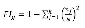
(4) where FIg is the level of social preference type heterogeneity in a group.
- 5.3
- While we focus on social preference types rather than ethnicity, language, or age, we expect a negative relationship between heterogeneity and welfare in keeping with the prior literature (e.g. Alesina et al. 1999; Alesina & La Ferrara 2000; Banerjee & Somanathan 2007; Costa & Kahn 2003; Miguel & Gugerty 2005; Vigdor 2004).
- 5.4
- We conduct the following analysis for four different weights on beliefs and preferences (in accordance with Fischbacher & Gächter 2010), as discussed in the previous section.
- 5.5
- To estimate the impact of social preference type heterogeneity group welfare, we estimate the following model:

(5) where g=1,…,G indexes groups, and t indicates the period. Cg,t is group g's average contribution to the public good in period t; Rt is the period; SPHg is level of social preference heterogeneity in group g; νg is the idiosyncratic random effect of group g, and eg,t is the error term. Further, ηl is the vector of coefficients of social preference types where l=1,…,9 indexes the type. Each of these controls is the number of each social preference type in the group and ranges from 0 to 4. Free riders are the omitted category, so all coefficients are interpreted as relative to a group of four Free riders. This allows straightforward comparison with the results put forward in traditional economic analysis, where all agents are assumed to be this type. Results are presented in Table 1, below.
- 5.6
- Model 1 presents the estimation results when contributions are fully preference driven (α=1).[6] In this model, we see that average group contributions decline over time. Social preference heterogeneity (SPH) is negative but not statistically significant.
- 5.7
- The preference controls are all positive and statistically significant (p < 0.0001). This is an artifact of using the traditional assumption of all free-riders as the omitted category. Moreover, these estimates are significantly different from each other (within each tested model). We will begin our discussion with the unconditional contribution preference types. For each free rider in a group that is replaced with a low contributor, overall contributions increase by 1.35 tokens (p < 0.0001). Each high contributor type increases contributions by 4.5 tokens. Maximum contributors have the highest impact on contributions at 5.86 tokens. Finally, noisy players positively impact contributions by 2.99 tokens.
- 5.8
- Among the conditional contribution preference types, economic altruists have the highest impact on contributions at 3.12 tokens, which is to be expected when average contributions are less than half of the maximum possible. Each conditional cooperator increases contributions by 2.88 tokens, while each hump player adds 1.94 tokens and each threshold player adds 2.71 tokens. We find that individuals with unconditional contribution preferences have, on average, a larger impact on average group contributions relative to free riders than conditional players do.
Table 1: Group Contributions a, b, c, d [1] [2] [3] [4] Preferences FG Model 3 FG Model 4a FG Model 4b-c α = 1
β = 0α = 0.242
β = 0.666α = 0.443
β = 0.545α = 0.385 {0.614}
β = 0.582 {0.376}Rt -0.043*** -0.258*** -0.383*** -0.443*** (0.001) (0.000) (0.002) (0.002) SPHe -0.036 -0.115* -1.350*** -1.503*** (0.070) (0.045) (0.211) (0.194) Low Contributors 1.348*** 0.540*** (0.019) (0.013) High Contributors 4.503*** 1.756*** (0.019) (0.013) Maximum Contributors 5.857*** 2.376*** (0.019) (0.013) Noisy Players 2.991*** 1.177*** (0.019) (0.013) Conditional Cooperators 2.875*** 0.993*** 1.696*** 1.610*** (0.019) (0.013) (0.041) (0.038) Economic Altruists 3.124*** 1.355*** (0.019) (0.013) Threshold Players 2.707*** 0.759*** (0.019) (0.013) Hump Players 1.938*** 0.800*** 1.397*** 1.367*** (0.019) (0.013) (0.041) (0.038) Constant -1.547*** 4.751*** 4.337*** 4.581*** (0.066) (0.047) (0.131) (0.121) Between R2 0.727 0.472 0.573 0.596 Within R2 0.006 0.497 0.738 0.739 Overall R2 0.634 0.477 0.605 0.634 Chi2 (P) 134067.1 (0.0) 483759.3 (0.0) 40036.0 (0.0) 40487.1 (0.0) Observations 495000 495000 15000 15000 a Random effects regressions. Dependent variable is average contributions to the public good by a group. b † 10%, * 5%, ** 1%, *** 0.1% significance level. c Standard errors in parentheses. d Model 1 estimates the equation for the fully preference driven model. Model 2-4 incorporate beliefs, and estimate the equation for Belief Model 3, Belief Model 4a, and Mixed Belief Model 4b-c, respectively. e Social Preference Heterogeneity, calculated using the fractionalization index. - 5.9
- In Model 2, we incorporate beliefs using the estimates from Fischbacher and Gächter (2010, their Model 3, α=0.242, β=0.666). When beliefs are incorporated into agents' contribution decisions independently of their preference type (that is β>0), preferences play a smaller role, and hence, their relative importance, as seen through the magnitude of the coefficients, drops substantially. As before, average group contributions decline over time. Now, however, SPH is negative and statistically significant.
- 5.10
- In Models 3 and 4, we restrict the sample to the three most common contribution preference types: free riders, conditional cooperators, and hump players. The α's and β's are chosen in accordance with Fischbacher and Gächter's (2010) Models 4a and 4b-c, as discussed in the previous section. For Model 4b-c, α=0.385 and β=0.582 for the first 5 rounds, and α=0.614 and β=0.376 for the last 5 rounds.
- 5.11
- We see that SPH is larger, negative and statistically significant. Further, as the weight on preferences (relative to beliefs) increases, the magnitude of the impact to contributions of replacing a free rider with either a conditional cooperator or a hump player is higher. For each conditional cooperator in the group, contributions increase by 1.6 to 1.7 tokens to (p<0.0001), and for each hump player, contributions increase by approximately 1.4 tokens (p<0.0001).
- 5.12
- Taken together, these results shed light on the importance of contribution preference types and beliefs on public good contributions. Certain preference types lead to more efficient groups than others. However, since SPH has a negative effect, the net effect of diversifying would be lower than expected.
Results: Robustness
- 6.1
- It is important to note that the coefficient estimate on the SPH is not always negative across our reported models: Is not significant in Model 1, which is the Fully Preference Driven model. This seems like a counterintuitive result, since heterogeneity in preferences is what comprises the SPH variable. Hence, as the weight on preferences in contribution decisions increases, one might expect that the coefficient on SPH should remain negative and significant. In order to investigate this, we conduct simulations identical to the models above, systematically changing the weights on beliefs and preferences.
- 6.2
- As previously mentioned, the parameters α, β are weights on the average of beliefs and preferences for contribution decisions. Our results estimate models based on the parameter estimates generated by the data collection exercise of Fischbacher and Gächter (2010). However, these weights are simply estimates, and thus may not be appropriate given the small samples used by the authors.[7] We thus extend our analysis by estimating additional models where we vary the values α, β. The only constraint we impose on the parameters is that they are contribution decision weights, and therefore, must sum to 1. Thus, we vary the strength of preferences and beliefs in the contribution decision of agents, from the fully preference driven model (as above: where α = 1 and β = 0) to the fully beliefs driven model (where α = 0 and β =1).
Table 2: Group Contributions – Free Riders, Conditional Cooperators, and Hump Playersa, b, c Panel A α = 0 α = .1 α = .2 α = .3 α = .4 α = .5 β = 1 β = .9 β = .8 β = .7 β = .6 β = .5 Rt -0.0222*** -0.115*** -0.185*** -0.230*** -0.268*** -0.299*** (0.00) (0.00) (0.00) (0.00) (0.00) (0.00) SPH d -0.132 -0.352* -0.640*** -1.218*** -1.225*** -2.173*** (0.23) (0.21) (0.19) (0.18) (0.17) (0.16) Conditional 1.187*** 1.420*** 1.656*** 1.882*** 2.014*** 2.162*** Cooperators (0.04) (0.04) (0.04) (0.03) (0.03) (0.03) Hump Players 1.084*** 1.373*** 1.544*** 1.740*** 1.901*** 2.023*** (0.04) (0.04) (0.03) (0.03) (0.03) (0.03) Constant 4.956*** 4.294*** 3.722*** 3.195*** 2.622*** 2.433*** (0.13) (0.10) (0.09) (0.08) (0.07) (0.07) Overall R2 0.313 0.467 0.578 0.675 0.741 0.770 Within R2 0.004 0.117 0.279 0.386 0.471 0.522 Between R2 0.371 0.523 0.625 0.720 0.785 0.811 Observations 15,000 15,000 15,000 15,000 15,000 15,000 Panel B α = .6 α = .7 α = .8 α = .9 α = 1 β = .4 β = .3 β = .2 β = .1 β = 0 Rt -0.314*** -0.331*** -0.337*** -0.342*** -0.341*** (0.00) (0.01) (0.01) (0.01) (0.01) SPH d -2.289*** -3.161*** -3.603*** -3.586*** -3.937*** (0.17) (0.15) (0.16) (0.15) (0.15) Conditional Cooperators 2.250*** 2.364*** 2.506*** 2.468*** 2.479*** (0.03) (0.03) (0.03) (0.03) (0.03) Hump Players 2.097*** 2.200*** 2.227*** 2.245*** 2.277*** (0.03) (0.03) (0.03) (0.03) (0.03) Constant 1.972*** 1.870*** 1.611*** 1.373*** 1.212*** (0.07) (0.06) (0.07) (0.07) (0.07) Overall R2 0.785 0.813 0.819 0.808 0.803 Within R2 0.532 0.549 0.535 0.495 0.469 Between R2 0.828 0.856 0.865 0.865 0.866 Observations 15,000 15,000 15,000 15,000 15,000 a Random effects regressions. Dependent variable is average contributions to the public good by a group. b † 10%, * 5%, ** 1%, *** 0.1% significance level. c Standard errors in parentheses. d Social Preference Heterogeneity, calculated using the fractionalization index. - 6.3
- Table 2, above, presents extends the analysis of the three contribution types used in models 4a and 4b-c: free-riders, conditional cooperators, and hump players. For each parameter estimate we have 15,000 observations.
- 6.4
- Each column presents estimation results for different values of α and β. For this analysis we restrict α and β to sum to 1, so that they are relative weights. The first column shows contribution decisions that are based purely on beliefs (α = 0 and β = 1). Each subsequent model increases the weight on α by 0.1 and reduces the weight on β by 0.1. This continues until the final column, where contribution decisions are purely based on preferences (α = 1 and β = 0).
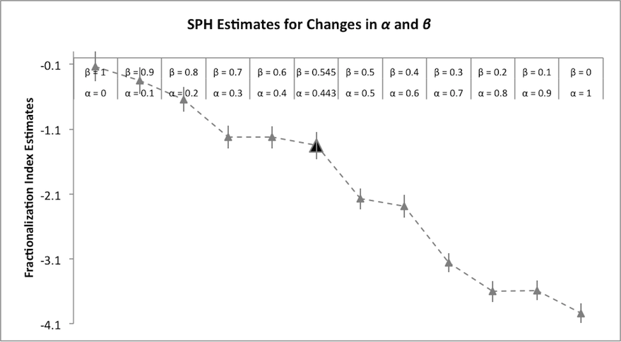
Figure 1. Changes in SPH Marginal Effects Sample Restricted to Free Riders, Conditional Cooperators, and Hump Players - 6.5
- Figure 1 contains the SPH marginal effects as a function of the relative weights. [8] The triangles represent the marginal effect for each set of relative weights, while the vertical bars display plus/minus one standard error. The larger, dark grey triangle depicts the estimates from Table 1.
- 6.6
- In Figure 1, note that only case where β = 1, and thus contributions are completely driven by beliefs, is the SPH parameter estimate not significant. This is consistent with our agents being homogeneous when α = 0. For each unit increase in the weight on preferences, the parameter on SPH becomes larger and more strongly significant[9]. For this model, the magnitude of the estimated effect is increasing in α. These results further point to the robustness of our findings to changes in parameter estimates for the most commonly observed types.
- 6.7
- Figure 2 repeats the analysis for all types of players, with the supporting regressions shown in Appendix Table A1.
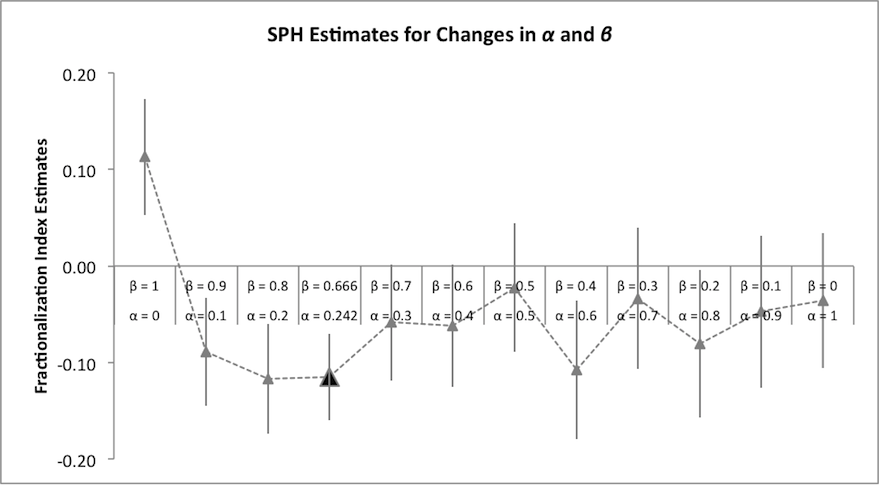
Figure 2. Changes in SPH Marginal Effects All Preference Types - 6.8
- For the full set of preference types, point estimates are generally negative but are only statistically significant in the parameter space surrounding the Fischbacher and Gächter estimates.
- 6.9
- We believe there are several reasons for the different effects between the models. First, the full set of social preference types includes more types which do not incorporate beliefs into their contribution preferences (thus, they do not condition Pit on the choices made by others). Thus, changing the weight on belief (β) impacts all players directly but only impacts a fraction of the agents' contribution preferences. This results in a u-shaped relationship between the weight on beliefs and actual contributions: Thus the social preference heterogeneity is only statistically significant for a portion of the parameter space.
- 6.10
- Second, these less-common (based on previous research) types are over-weighted in our data in comparison with either naturally-occurring or experimentally-generated data. In order to focus on heterogeneity and use the power of simulation to gather information on how groups with these types behave we have, by construction, treated the likelihood of encountering one of these players as equal to encountering, say, a conditional cooperator. This has the advantage of providing a very strong stress-test of the model but the disadvantage of being less reflective of actual societies.
- 6.11
- We thus find that social preference heterogeneity significantly and strongly impacts group welfare in a number of plausible settings but is by no means a foregone conclusion. We now turn to our closing discussion.
Closing Discussion
- 7.1
- We conduct an agent-based simulation of individual contributions to public goods. We identified nine distinct preference types in the literature, and constructed agents to be simulated based on these types. We then allowed agents to be configured with beliefs, and utilized those respectively updated values to calculate contributions in each simulated period based on the findings of Fischbacher and Gächter (2010). We then systematically varied the composition for 4-agent groups playing a public goods game. We find the traditional decay in contributions and that unconditional contributors have a higher impact on contributions than conditional types.
- 7.2
- A large stream of literature demonstrates a negative relationship between various types of heterogeneity and public goods provision (Alesina et al. 1999; Miguel & Gugerty 2005; Vigdor 2004). We complement this literature by investigating a different type of heterogeneity: social preference heterogeneity. We find that heterogeneity in intrinsic factors (i.e. the type of social preferences agents hold) may also negatively impact the voluntary provision of public goods. In particular, we find that varying the social preference heterogeneity of the group impacts efficiency, or welfare, in some settings but not in others. Specifically, social preference heterogeneity strongly impacts group contributions when the groups are restricted to the most common social preference types, but only significantly for a small range of the parameter space when all types are considered. We believe this is due to the tradeoff between the direct impact of beliefs and the combined impact of agent type and the indirect influence of beliefs for conditional types.
- 7.3
- Interesting future work in this area could address the role of punishment as well as the relationship between the propensity to engage in punishment and an agent's social preference type. Additional future work in this area should focus on examining various models of belief formation, and to also allow beliefs to vary according to preference types. Finally, an interesting unresolved question is whether or not observable factors reported in the literature (race, ethnicity, income, language, etc.) are correlated with different underlying social preference types.
- 7.4
- The designed agent-based experiment allowed the systematic analysis of how different group compositions and individual social preference heterogeneity affect contributions in a public goods game setup. We have discussed a computational model that has been developed to provide a flexible tool to test, via simulations, experimentally observed behaviours under different circumstances.
Appendix
-
Table A1: Group Contributions – All Types a, b, c. To accompany Figure 2. Panel A. α = 0 α = .1 α = .2 α = .3 α = .4 α = .5 β = 1 β = .9 β = .8 β = .7 β = .6 β = .5 Rt -0.148*** -0.131*** -0.114*** -0.0999*** -0.0874*** -0.0807*** (0.00) (0.00) (0.00) (0.00) (0.00) (0.00) SPHd 0.113* -0.089 -0.117** -0.059 -0.062 -0.022 (0.06) (0.06) (0.06) (0.06) (0.06) (0.07) Types: Conditional 1.104*** 1.467*** 1.745*** 1.970*** 2.152*** 2.334*** Cooperators (0.02) (0.01) (0.01) (0.01) (0.01) (0.01) Maximum 2.213*** 2.985*** 3.588*** 4.123*** 4.534*** 4.870*** Contributors (0.01) (0.01) (0.01) (0.01) (0.01) (0.01) Low Contributors 0.484*** 0.679*** 0.818*** 0.959*** 1.032*** 1.116*** (0.01) (0.01) (0.01) (0.01) (0.01) (0.01) High Contributors 1.651*** 2.238*** 2.707*** 3.067*** 3.386*** 3.671*** (0.02) (0.01) (0.01) (0.01) (0.01) (0.01) Economic Altruists 1.100*** 1.532*** 1.855*** 2.146*** 2.359*** 2.558*** (0.02) (0.01) (0.01) (0.01) (0.01) (0.01) Noisy Players 1.102*** 1.512*** 1.792*** 2.064*** 2.258*** 2.453*** (0.02) (0.01) (0.01) (0.01) (0.01) (0.01) Threshold Players 1.102*** 1.417*** 1.670*** 1.889*** 2.034*** 2.163*** (0.02) (0.02) (0.02) (0.02) (0.02) (0.02) Hump Players 1.111*** 1.387*** 1.582*** 1.774*** 1.861*** 1.984*** (0.02) (0.01) (0.01) (0.01) (0.01) (0.01) Constant 5.646*** 4.224*** 3.046*** 1.978*** 1.206*** 0.494*** (0.05) (0.05) (0.04) (0.04) (0.04) (0.05) Overall R2 0.308 0.479 0.578 0.627 0.654 0.665 Within R2 0.185 0.170 0.123 0.083 0.055 0.040 Between R2 0.329 0.520 0.630 0.686 0.719 0.735 Observations 495,000 495,000 495,000 495,000 495,000 495,000 a Random effects regressions. Dependent variable is average contribution to the public good by a group. b † 10%, * 5%, ** 1%, *** 0.1% significance level. c Standard errors in parentheses. d Social Preference Heterogeneity, calculated using the standard fractionalization index. Table A1: Continued a, b, c: Panel B α = .6 α = .7 α = .8 α = .9 α = 1 β = .4 β = .3 β = .2 β = .1 β = 0 Rt -0.0713*** -0.0669*** -0.0590*** -0.0535*** -0.043*** (0.00) (0.00) (0.00) (0.00) (0.00) SPHd -0.108 -0.034 -0.081 -0.047 -0.036 (0.07) (0.07) (0.08) (0.08) (0.07) Types: Conditional 2.438*** 2.548*** 2.629*** 2.705*** 2.875*** Cooperators (0.01) (0.02) (0.02) (0.02) (0.02) Maximum 5.152*** 5.370*** 5.560*** 5.704*** 5.857*** Contributors (0.01) (0.01) (0.01) (0.01) (0.02) Low Contributors 1.174*** 1.213*** 1.271*** 1.315*** 1.348*** (0.01) (0.01) (0.01) (0.01) (0.02) High Contributors 3.866*** 4.065*** 4.187*** 4.314*** 4.503*** (0.01) (0.01) (0.01) (0.01) (0.02) Economic Altruists 2.712*** 2.811*** 2.947*** 3.045*** 3.124*** (0.01) (0.01) (0.01) (0.01) (0.02) Noisy Players 2.601*** 2.696*** 2.798*** 2.886*** 2.991*** (0.01) (0.01) (0.01) (0.01) (0.02) Threshold Players 2.300*** 2.354*** 2.471*** 2.515*** 2.707*** (0.03) (0.03) (0.03) (0.03) (0.02) Hump Players 2.027*** 2.059*** 2.099*** 2.113*** 1.938*** (0.01) (0.01) (0.01) (0.01) (0.02) Constant (0.00) -0.434*** -0.820*** -1.144*** -1.547*** (0.05) (0.05) (0.05) (0.06) (0.07) Overall R2 0.668 0.669 0.664 0.656 0.727 Within R2 0.028 0.021 0.015 0.010 0.006 Between R2 0.741 0.746 0.746 0.744 0.634 Observations 495,000 495,000 495,000 495,000 495,000 a Random effects regressions. Dependent variable is average contribution to the public good by a group. b † 10%, * 5%, ** 1%, *** 0.1% significance level. c Standard errors in parentheses. d Social Preference Heterogeneity, calculated using the standard fractionalization index.
Acknowledgements
- We would like to thank Laura Ahmadi and Abdul Kidwai for providing research assistance on this project. Additionally we would like to thank the Dynamics Lab, at the University College Dublin, for having provided access to the server, on which we have run the experiments. Views expressed here are not necessarily those of the World Bank or its member governments.
Notes
-
1 Heterogeneity or fractionalization is generally measured using the ethnolinguistic fractionalization index, ELF, which is one minus the Herfindahl index of group shares. In a population that is completely homogeneous, it takes on a value of zero. In a population that is completely fractionalized, it takes on a theoretical maximum of one. The interpretation of the variable is the probability that two randomly selected individuals in the population will belong to separate ethnolinguistic groups (Easterly & Levine 1997).
2 This is also referred to as unconditional commitment (see Collard 1978; Sudgen 1984).
3 Note that the economic definition of altruism differs substantially from that used in other circles. We will employ the term in keeping with the economics profession, as described in more detail in the next section. Under this definition, others' welfare is essentially a public good which an individual wants provided but whose own contributions are crowded out by the contributions of others.
4 The linear voluntary contribution mechanism (VCM), which is generically referred to as the public goods game, was first studied experimentally in Marwell and Ames (1979) and has been systematically reviewed since then. For systematic reviews of the literature, see Chaudhuri (2011), Davis and Holt (Chapter 6, 1994), Ledyard (1995), and Zelmer (2003).
5 Further, we do not allow first-round beliefs to vary by type, though there is some evidence to suggest that it would be an interesting extension in further work (e.g. Orbell & Dawes 1993).
6 Note that beliefs still impact behavior indirectly through Pit for each type of player where δi≠0.
7 We would like to thank an anonymous referee for suggesting this analysis.
8 These agent types (free riders, conditional cooperators and hump/triangle players) make up 90% of all player types, as reported in Fischbacher and Gächter (2010).
9 The figure also includes (as a reference point) the parameter reported in table 1 using Fischbacher and Gächter's model 4.
References
-
ALESINA, A., Baqir, R. & Easterly, W. (1999). 'Public Goods and Ethnic Divisions.' Quarterly Journal of Economics. 114(4): 1243–1284. [doi:10.1162/003355399556269]
ALESINA, A., Devleeschauwer, A., Easterly, W., Kurlat, S. & Wacziarg, R. (2003) 'Fractionalization.' Journal of Economic Growth. 8: 155–194. [doi:10.1023/A:1024471506938]
ALESINA, A. & La Ferrara, E. (2000). 'Participation in Heterogeneous Communities.' Quarterly Journal of Economics. 115(3): 847–904. [doi:10.1162/003355300554935]
AHN, T.K., Ostrom, E. & Walker, J. M. (2003). 'Heterogeneous Preferences and Collective Action.' Public Choice. 117(3–4): 295–314.
ANDREONI, J. (1989). 'Giving with Impure Altruism: Applications to Charity and Ricardian Equivalence.' Journal of Political Economy. 97: 1447–1458.
ANDREONI, J. (1990). 'Impure Altruism and Donations to Public Goods: A Theory of Warm-Glow Giving.' Economic Journal. 100: 464–477.
BANERJEE, A. & Somanathan, R. (2007). 'The Political Economy of Public Goods: Some Evidence from India.' Journal of Development Economics. 82(2): 287–314. [doi:10.1016/j.jdeveco.2006.04.005]
BECKER, G.S. (1974). 'A Theory of Social Interactions.' Journal of Political Economy.' 82(6): 1063–93. [doi:10.1086/260265]
BESLEY, T. & Ghatak, M. (2006). 'Public Goods and Economic Development.' In Banerjee, A.V., Bénabou, R. & Mookherjee, D. (eds.) Understanding Poverty. Oxford: Oxford University Press. Chapter 19. pp. 285–302.
BURLANDO, R. M. & Guala, F. (2005). 'Heterogeneous Agents in Public Goods Experiments.' Experimental Economics. 8(1): 35–54 [doi:10.1007/s10683-005-0436-4]
CAMERER, C. & Fehr, E. (2004). 'Measuring Social Norms and Preferences Using Experimental Games: A Guide for Social Scientists.' In Foundations of Human Sociality: Economic Experiments and Ethnographic Evidence from Fifteen Small-Scale Societies. Oxford and New York: Oxford University Press. pp. 55–95.
CHARNESS, G. & Rabin, M. (2002). 'Understanding Social Preferences with Simple Tests.' Quarterly Journal of Economics. 117(3): 817–869. [doi:10.1162/003355302760193904]
CHAUDHURI, A. (2011). 'Sustaining Cooperation in Laboratory Public Goods Experiments: A Selective Survey of the Literature.' Experimental Economics. 14(1): 47–83. [doi:10.1007/s10683-010-9257-1]
CHEN, L.C., Evans, T.G. & Cash, R.A. (1999). 'Health as a Global Public Good.' In I. Kaul, I. Grunberg and M.A. Stern (eds.). Global Public Goods: International Cooperation in the 21st Century. Published for The United Nations Development Programme. Oxford: Oxford University Press.
COLLARD, D. (1978) Altruism and Economy. Oxford: Martin Robertson.
CORNES, R. & Sandler, T. (1996). The Theory of Externalities, Public Goods and Club Goods, 2nd ed. Cambridge: Cambridge University Press. [doi:10.1017/CBO9781139174312]
COSTA, D.L. & Kahn, M.E. (2003). 'Civic Engagement and Community Heterogeneity: An Economist's Perspective.' Perspectives on Politics. 1: 103–111.
CROSON, R.T.A. (2007). 'Theories of Commitment, Altruism and Reciprocity: Evidence from Linear Public Goods.' Economic Inquiry. 45(2): 199–216. [doi:10.1111/j.1465-7295.2006.00006.x]
DAVIS, D. & Holt, C. (1994). Experimental Economics. Princeton: Princeton University Press.
DE OLIVEIRA, A.C.M., Eckel, C. & Croson, R.T.A. (2013). 'One Bad Apple? Heterogeneity and Information in Public Goods Provision.'
EASTERLY, W. (2001). 'Can Institutions Resolve Ethnic Conflict?' Economic Development and Cultural Change. 49(4): 687–706. [doi:10.1086/452521]
EASTERLY, W. & Levine, R. (1997). 'Africa's Growth Tragedy: Policies and Ethnic Divisions.' Quarterly Journal of Economics. 112(4): 1203–1250.
FAN, S., Hazell, P. & Thorat, S. (1999). 'Linkages between Government Spending, Growth, and Poverty in Rural India.' IPFRI Research Report No. 110.
FAN, S., Zhang, L. & Zhang, X. (2002). 'Growth, Inequality, and Poverty in Rural China: The Role of Public Investments.' IFPRI Research report No. 125.
FEHR, E. & Fischbacher, U. (2002). 'Why Social Preferences Matter – The Impact of Non-Selfish Motives on Competition, Cooperation and Incentives.' The Economic Journal. 112(478): C1–C33.
FEHR, E. and Gächter, S. (2000). 'Fairness and Retaliation: The Economics of Reciprocity.' Journal of Economic Perspectives. 14(3): 159–181. [doi:10.1257/jep.14.3.159]
FISCHBACHER, U. & Gächter, S. (2010). 'Social Preferences, Beliefs, and the Dynamics of Free Riding in Public Goods Experiments.' American Economic Review. 100(1): 541–556. [doi:10.1257/aer.100.1.541]
FISCHBACHER, U., Gächter, S. & Fehr, E. (2001). 'Are People Conditionally Cooperative? Evidence from a Public Goods Experiment.' Economics Letters. 71(3): 397–404. [doi:10.1016/S0165-1765(01)00394-9]
FREY, B. S. & Meier, S. (2004). 'Social Comparisons and Pro-Social Behavior: Testing 'Conditional Cooperation' in a Field Experiment.' American Economic Review. 94(5): 1717–1722.
GÄCHTER, S. (2007). 'Conditional Cooperation: Behavioral Regularities from the Lab and the Field and Their Policy Implications.' In Frey, B.S. & Stutzer, A. (eds.). Psychology and Economics: A Promising New Cross-Disciplinary Field. Cambridge, MA: MIT Press. pp. 19–50.
GÄCHTER, S. & Thöni, C. (2005). 'Social Learning and Voluntary Cooperation among Like-Minded People.' Journal of the European Economic Association. 3(2–3): 303–314.
HARDIN, G. (1968) 'The Tragedy of the Commons.' Science. 162(3859): 1243–1248. [doi:10.1126/science.162.3859.1243]
HENRICH, J., Boyd, R., Bowles, S., Camerer, C., Fehr, E., Gintis, H. & McElreath, R. (2001). 'In Search of Homo Economicus: Behavioral Experiments in 15 Small-Scale Societies.' American Economic Review, Papers and Proceedings. 91(2): 73–78. [doi:10.1257/aer.91.2.73]
HERRMANN, B. & Thöni, C. (2009). 'Measuring Conditional Cooperation: A Replication Study in Russia.' Experimental Economics. 12(1): 87–92. [doi:10.1007/s10683-008-9197-1]
KURZBAN, R. & Houser, D. (2005). 'Experiments Investigating Cooperative Types in Humans: A Complement to Evolutionary Theory and Simulations.' PNAS. 102(5): 1803–1807. [doi:10.1073/pnas.0408759102]
LABAREE, D.F. (1997). 'Public Goods, Private Goods: American Struggle Over Educational Goals.' American Educational Research Journal. 34(1): 39–81. [doi:10.3102/00028312034001039]
LEDYARD, J. (1995). 'Public Goods: A Survey of Experimental Research.' In Kagel, J. & Roth, A. (Eds.), The Handbook of Experimental Economics. Princeton: Princeton University Press.
MATSUMOTO, M. & Nishimura, T. (1998). Mersenne twister: a 623-dimensionally equidistributed uniform pseudo-random number generator. ACM Trans. Model. Comput. Simul. 8, 1, 3–30. [doi:10.1145/272991.272995]
MARWELL, G. & Ames, R. (1979). 'Experiments on the Provision of Public Goods I: Resources, Interest, Group Size and the Free-Rider Problem.' American Journal of Sociology. 84: 1335–1360.
MAURO, P. (1995). 'Corruption and Growth.' Quarterly Journal of Economics. 110(3): 681–712. [doi:10.2307/2946696]
MIGUEL, E. (2004). 'Tribe or Nation? Nation-Building and Public Goods in Kenya versus Tanzania.' World Politics. 56(3): 327–362. [doi:10.1353/wp.2004.0018]
MIGUEL, E. & Gugerty, M.K. (2005). 'Ethnic Diversity, Social Sanctions, and Public Goods in Kenya.' Journal of Public Economics. 89(11–12): 2325–2368.
OLSON, M. (1965). The Logic of Collective Action: Public Goods and the Theory of Groups. Cambridge, MA: Harvard University Press.
ORBELL, J. M. and R. M. Dawes (1993). 'Social Welfare, Cooperators' Advantage, and the Option of Not Playing the Game.' American Sociological Review. 58(6): 787–800.
POTERBA, James M. (1997). 'Demographic Structure and the Political Economy of Public Education.' Journal of Policy Analysis and Management. 16(1): 48–66. [doi:10.1002/(SICI)1520-6688(199724)16:1<48::AID-PAM3>3.0.CO;2-I]
ROTH, A. E., Prasnikar, V., Fujiwara, M. & Zamir, S. (1991). 'Bargaining and Market Behavior in Jerusalem, Ljubljana, Pittsburgh, and Tokyo: An Experimental Study.' American Economic Review. 81(5): 1068–1095.
SHAFIK, N. (1994). 'Economic Development and Environmental Quality: An Econometric Analysis.' Oxford Economic Papers. 46: 757–773.
SQUIRE, L. (1993). 'Fighting Poverty.' American Economic Review. 83(2): 377-382.
SUDGEN, R. (1984). 'Reciprocity: The Supply of Public Goods through Voluntary Contributions.' Economic Journal. 94: 772–787.
VIGDOR, J.L. (2004). 'Community Composition and Collective Action: Analyzing the Initial Mail Response to the 2000 Census.' Review of Economics and Statistics. 86(1): 303–312. [doi:10.1162/003465304323023822]
WORLD BANK (1990). Poverty-World Bank Development Report 1990. Washington, DC: World Bank.
ZAK, P.J. & Knack, S. (2001). 'Trust and Growth' The Economic Journal. 111(470): 295–321. [doi:10.1111/1468-0297.00609]
ZELMER, J. (2003). 'Linear Public Goods: A Meta-Analysis.' Experimental Economics. 6(3): 299–310. [doi:10.1023/A:1026277420119]