
 Abstract
- The morphological properties of genealogical and marriage alliance networks constitute a key to the understanding of matrimonial behavior and social norms, in particular where these norms have not been explicitly formalized. Their analysis, however, faces a major difficulty: the actual datasets which allow researchers to reconstruct kinship and alliance networks are generally subject to a marked observer bias, if only due to limitations of observer mobility and/or informant memory. This paper presents an agent based simulation method destined to evaluate the impact of this bias on some key indicators of kinship and alliance networks (such as matrimonial circuit frequencies). The method consists in explicitly simulating the exploration of a given network by a virtual observer, the bias being introduced by the observer's inclination for choosing informants who are more or less closely related to each other. The article presents the model for genealogical and for alliance networks, applies it to a series of artificial networks exhibiting some characteristic morphological patterns, and discusses the divergence of observed from real patterns for different kinds and degrees of observer bias. The methods presented have been implemented in the free software Puck 2.0.
- Keywords:
- Kinship, Marriage Alliance, Agent Based Simulation, Observer Bias, Fieldwork, Ebrei
Introduction
- 1.1
- The morphological properties of social networks emerge from the interaction of local choices according to behavioral patterns that range from individual preferences to formalized social norms. Their analysis constitutes a key method to grasp these underlying behavioral patterns, in particular where formalized norms do not exist or are not necessarily followed in practice. A long-standing example for this method is the technique of anthropologists and historians of the family to use the relative numbers of marriages between kin or affine of certain types – in other terms, a census of matrimonial circuits in kinship networks (White & Jorion 1992; Hamberger 2011) – as indicators for matrimonial preferences or avoidances. Thus, for example, a high number of marriages between patrilateral parallel cousins combined with a low number of marriages with matrilateral parallel cousins may be (and frequently is) interpreted as indicating a preference for marrying the former and an avoidance against marrying the latter.
- 1.2
- For a long time restricted to the study of close cousin marriages in small genealogies, this method has gained considerable importance since computer tools have made it possible to effectuate exhaustive censuses for a virtually unbounded number of circuit types in large kinship networks (see Barry 2004; White et al. 1999; Hamberger et al. 2014). This technological progress seemed to open completely new perspectives to the comparative study of kinship and marriage structures: the study of what people say about marriage (incest prohibitions, prescriptive kinship terminologies, etc.) could now be confronted with large-scale statistical analyses of what people really do.
- 1.3
- This research program, however, faces a serious obstacle: the collection of genealogical data is often heavily biased by factors which pertain as much to the observer's research objectives and conditions (including budget) as to the social structure, including kinship and marriage links – that is, precisely the phenomena one wants to study. For example, an ethnographer with a restricted transport budget doing genealogical research in a patri-virilocal society (where women reside with their husband's paternal kin) necessarily will gather less information on matrilateral than on patrilateral links, and therefore is likely to underestimate marriages between matrilateral relatives. The situation may even be worse for the historian who has to rely on the data collected by a 17th century notary who systematically omitted information on wives' parents, so that even a generous research budget would not allow him or her to search the matrilateral kin in the archives of neighboring towns. As a consequence, the morphological features of observed social networks emerge as the joint product of two quite different kinds of behavior: the matrimonial behavior of the agents we want to study, and the behavior of the observer(s) who collected the data. Kinship networks tell us always (at least) two stories at the same time, and in order to read them properly, we have to try to separate them.
- 1.4
- In this paper, we will show how agent-based simulation of observer behavior ("Virtual Fieldwork") can be used to address this issue. Although simulation techniques have been used to study matrimonial structures since the 1960s (Kunstadter et al. 1963; Gilbert & Hammel 1966; Fischer 1986, 1994, 2006; Read 1998; Small 2000; Geller et al. 2011), they have never been used to explicitly study observer bias, and the only study that addresses this issue (White 1999) does not use an agent-based model. The model which we present in this paper in order to study a concrete problem of empirical anthropology and family history may thus reveal itself a fruitful instrument in many other areas of social network theory (see Gargiulo and Roth (s.d.) for an application of the "alliance network" version of the model to web mining algorithms).
- 1.5
- We will start by introducing the basic notions of kinship and alliance networks and present the problem of interpreting matrimonial circuit censuses, drawing on an empirical example. We shall then present the virtual fieldwork model, which we apply both to genealogical and to alliance networks. We will show that observer behavior, even if as neutral and objective as possible but subject to constraints related to the examined kinship system (such as residence rules), may lead to a bias which not only distorts the "brute" data but also the more subtle indicators we may hope to construct from them, such as potential or expected circuits. In the conclusions, we will address the questions how, in spite of these difficulties, we may still use genealogical datasets to study matrimonial practices.
The problem: How to read kinship networks?
-
Kinship and alliance networks
- 2.1
- Marriage ties link both individuals and groups. In kinship networks, marriage ties are between individuals who are also linked with each other by chains of parent-child ties. In alliance networks, marriage ties are between the groups to which the respective spouses belong (be they kinship groups like lineages or clans, residential, professional, or other kinds of groups). More formally, we can define the two types of networks as follows:
- 2.2
- Kinship (or genealogical) networks are weakly acyclic mixed graphs where nodes represent individuals, arcs represent filiation ties (directed from parent to child nodes), and edges represent marriages[1].
- 2.3
- Alliance networks are oriented multigraphs, where nodes represent groups of individuals, and arcs represent (possibly multiple) marriages, directed from wife-givers to wife-takers[2]. An alliance network composed by m nodes (groups) and n directed links (marriages) can be represented by a weighted alliance matrix (xij), where xij is the number of marriage links connecting wife group i and husband group j.
- 2.4
- To illustrate these concepts, let us consider a dataset collected by Michael Gasperoni (2011, 2013), drawing on the matrimonial practices of Jewish families in early modern central Italy ("Ebrei", downloadable at www.kinsources.net/[3]). The genealogical network (figure 1a) contains 2597 marriages (edges) for 7331 individuals (nodes), distributed over 15 generations. From this network we can derive the alliance network of patrilineal components (figure 1b), where the same marriages (arcs) are distributed between 1740 patrilineal groups (nodes).
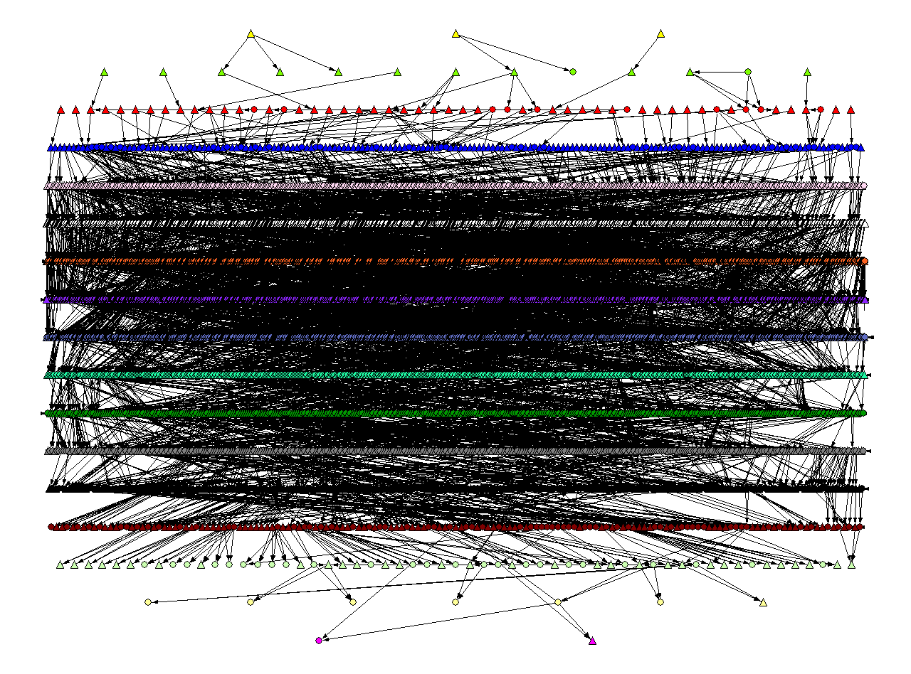
Figure 1a. Ebrei genealogical network. Visualization with Pajek. 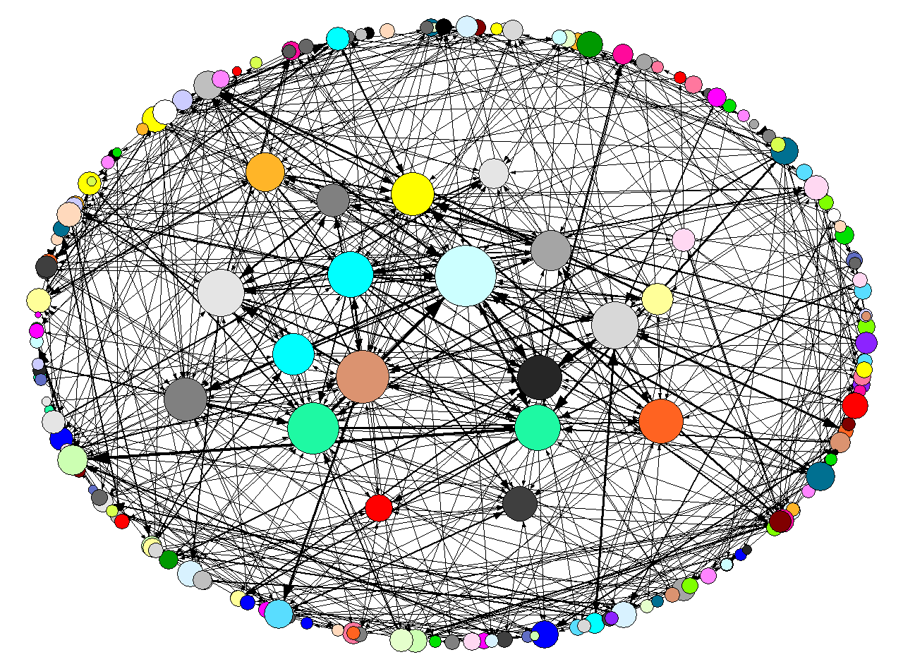
Figure 1b. Alliance network of the patrilineal components of the Ebrei dataset. To improve visibility, we have only represented nodes with more than 5 links. Visualization with Pajek. The circuit census
- 2.5
- To analyze the morphology of these networks, we effectuate a census of matrimonial circuits (see Hamberger et al. 2011). In genealogical networks, a matrimonial circuit is defined as a closed chain of kinship and marriage links in which no individual appears twice, and no individual is linked to two parents (a simple parent-child-triangle thus does not in itself constitute a matrimonial circuit). It follows from this definition that a matrimonial circuit contains at least one marriage link. Matrimonial circuits can thus be interpreted as kinship and marriage chains between spouses – their relative frequencies serving as potential indicators of matrimonial behavior.
- 2.6
- Clearly, the probability of a circuit to be formed depends not only on the preferences of individuals but also on the availability of chains of the given type. We will therefore not only look at the number of actually formed circuits, but also at the number of potential circuits, that is, open kinship and marriage chains between married people of opposite sex (potential spouses). The ratio of the number of closed kinship chains to the total number of chains of the given type (the closure rate of this type of chain) can serve as an indicator of the probability for relatives of a given kind to be married with each other.
- 2.7
- Table 1 shows the result of a simple matrimonial census for the Ebrei genealogical network, restricted to marriages between first cousins (that is, children of siblings): agnatic (related by male links only), uterine (related by female links only) and cognatic (related by mixed chains of male and female links).
Table 1: Matrimonial circuit frequencies and closure rates in the Ebrei network.
TypeCousin Marriages Normalized Total Chains Per Individual Closure Rate Agnatic 75 2.89% 1,404 0.38 5.34% Cognatic 53 2.04% 1,523 0.42 3.48% Uterine 21 0.81% 387 0.11 5.43% Total 141 5.43% 3,314 0.9 4.25% - 2.8
- The census yields a total of 141 first cousin marriages (5.4% of all marriages), some of which may be linked by more than one cousin relation at once. More than 50% of these marriages (75) are with the agnatic cousin (the father's brother's daughter) while only 14% (21) are with the uterine cousin (the mother's sister's daughter). However, due to the strong dominance of agnatic over uterine cousin relations in the network (53% vs 15% of all first cousin relations), closure rates are roughly the same (about 5%), and even somewhat higher for uterine chains.
- 2.9
- In the case of alliance networks, the circuit census is a simpler affair, as circuits here do not include any parent-child links, being simply closed chains of marriage arcs. In particular, we are interested in loops (which represent endogamous marriages) and dual circuits (which represent marriage relinkings). As only one type of arc is concerned, their numbers can be expressed in a straightforward manner. Using the matrix notation given above (where xij is the number of marriages between women of group i and men of group j, and n is the total number of marriages), the normalized number of endogamous marriages (loops) is given as

(1) and the normalized number of relinking marriages (dual circuits) as
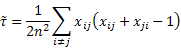
(2) - 2.10
- As in the case of genealogical networks, we are also interested in the potential number of circuits. In alliance networks, this number does not depend on consanguineous chains in the network, but on the matrimonial "strengths" of the nodes, that is, the numbers of spouses given and taken by each group[4]. Adopting a multinomial approach which estimates the probability of a random marriage link between two groups as directly proportional to their respective matrimonial strengths, expected circuit numbers can be calculated from matrimonial strength vectors (for details see Roth et al. 2013). Table 2 presents the results of a simple circuit census for the Ebrei alliance network:
Table 2: Circuit census for the Ebrei alliance network: actual and expected numbers of loops and dual circuits, both in absolute values and normalized by the maximal number of possible loops and relinkings. The last column gives the ratio of the former to the latter.
Typeactual (normalized) expected (normalized) divergence Loops (endogamous marriages) 128 0.04929 8.74 0.00336 14.65 Dual circuits (marriage relinkings) 364 0.00011 82.56 0.00002 4.41 - 2.11
- We see that the number of endogamous marriages (loops), roughly 5% of all marriages, is almost 15 times higher than what would be expected if the probability of a marriage between groups depended only on the number of male and female marriages concluded by each.
Interpreting the figures
- 2.12
- What can we conclude, from these figures, concerning the matrimonial practices of Jewish individuals and communities in early modern central Italy?
- 2.13
- The genealogical network shows a very high proportion of agnatic marriages. Moreover, there is evidence that the agnatic relations between spouses are considerably underestimated. In many cases, for example, the paternal relative who acted as a witness for the bride's waiving her rights of succession bears the same patronym as her husband, making it clear that the couple was paternally related, even if no genealogical chain could be established. In short, a first glance interpretation of these findings would suggest that the individuals constituting the network preferred marriage between close agnatic relatives – which is consistent with the literature on Jewish matrimonial rules (see Heymann 1994; Gasperoni 2013).
- 2.14
- However, this conclusion is called into question as soon as we look at closure rates, which no longer show any agnatic preponderance, due to the considerable over-representation of agnatic chains in the network. As demographic causes (such as polygamy) cannot account for this feature, there is obviously a marked observer bias in favor of male links.
- 2.15
- This "agnatic bias" can be explained by the particular conditions of data collection. Gasperoni's corpus had to be constructed from notarial documents of quite heterogeneous nature. On the one hand, wills, often delineating extended genealogical networks; on the other hand, dowry receipts (that is, marriage contracts), established by the notary of the husband's town, which often mentioned only the father of each spouse. The genealogical memory of a given informant (legator or spouse) "interviewed" by the 17th century observer (the notary) thus varied from quite extensive to extremely reduced, and in both cases showed an agnatic bias. A similar bias characterized the position of the observer himself. Before 1634, when all Jewish communities in the region were forced into four urban ghettos, they lived in communities which were organized in relatively small households, several of which were agnatically related with each other (residence being patri-virilocal, that is, with the husband's paternal relatives). Despite the comprehensive perspective of the 21th century observer, then, his material, shaped by the perspective of his 17th century predecessor, draws on information by people who were frequently close agnatic kin.
- 2.16
- Thus relativized, the new figures might prompt us to fall in the opposite extreme, and to claim that the divergences we observe in cousin marriage numbers should be ascribed altogether to residence rules and notarial usages. This sort of conclusion, however, presupposes that closure rates are themselves independent of observer bias, a hypothesis that cannot be assumed to be true (see Barry & Gasperoni 2008). In fact, kinship ties between spouses have a higher probability to be known than kinship chains that are not linking spouses, and this bias in favor of matrimonially "closed" (rather than "open") cousin relationships is further enforced by the fact that marriage is correlated with co-residence. The question is whether the agnatic bias affects the numbers of detected agnatic and uterine cousin marriages in the same way it affects the overall numbers of detected agnatic and uterine cousin relations.
- 2.17
- Quite the same considerations hold for the interpretation of circuit patterns in alliance networks. If we look at the alliance network of patrilineal components, we find a surplus of observed over expected endogamy which reveals a strong tendency towards marriages with agnatic relatives. However, as noted above, expectations are calculated from matrimonial strengths, the distribution of which is strongly distorted by the limited mobility of the observer. In order to draw any conclusions from our findings, we need to know the relative impact of this observer bias on observed and expected circuit frequencies.
- 2.18
- In summary, we thus have to address two fundamental questions: How does the observer's propensity to choose informants who are agnatic relatives of each other affect the relative frequencies of agnatic cousin relations and agnatic cousin marriages observed in genealogical networks, and how does it affect the distribution of marriages across agnatic groups and across pairs of agnatic groups in alliance networks?
- 2.19
- The method we suggest to address these questions is to explicitly simulate the observation process by a model of "Virtual Fieldwork", with a virtual observer navigating in the (kinship or alliance) network and extracting information from a series of virtual informants (individuals or groups).
- 2.20
- Since the models for genealogical and for alliance networks are very similar (though not identical), we shall present their general characteristics in the section concerned with genealogical networks, while the section on alliance networks will focus on the differences.
- 2.21
- Both models have been implemented in the free software Puck 2.0. (download at http://www.kintip.net/). The source code is available at http://sourceforge.net/projects/tip-puck/[5].
Virtual fieldwork in genealogical networks
-
The model
- 3.1
- The aim of the Virtual Fieldwork model is to explore the effects of observer and informant behavior on the overall morphology of the observed part of the kinship network. It is designed for theoretical exploration, not to reproduce the exact morphology of given networks.
Parameters and state variables
- 3.2
- The model comprises two types of networks—the real and the observed kinship network – and two types of agents – informants and the observer. The real kinship network consists of individuals and the links between them. As has been specified above, there are two kinds of links (parent-child and marriage links). This network will not change during the virtual fieldwork process. A subset of the individuals of the network constitutes the potential informants from which the actual informants are chosen by the observer. The limits of this subnetwork may be determined by space and time constraints. As we shall model spatial constraints by the observer's preferences for "close" informants (see below), the only a priori limitations to an individual's accessibility as an informant are temporal in nature (for instance, the condition of being the observer's contemporary). In what follows, we assume that the observer chooses individuals from the lowest age layer.
- 3.3
- The observed kinship network is a subnetwork of the real kinship network, which is reconstructed by the virtual fieldwork process from information given to the observer by the informants. The observed network thus changes at each time step[6].
- 3.4
- The observer, who is not part of the network, is characterized by a preference for choosing informants according to their network position (the only characteristics by which they differ). We assume that the only factor determining this choice is the new informant's network distance from the previous informant. Observer behavior thus is characterized by a sort of relational "inertia". The rationale for this assumption is that the availability and accessibility of informants often depend on their links with previous informants. Even without thinking of a snowballing strategy, this dependence may simply be due to the observer's mobility constraints, combined with the fact that spatial proximity is often correlated with certain kinship ties. Relatives that live closer together will have a higher chance to be interviewed by an observer who cannot afford to visit each and every living individual recorded during previous interviews.
- 3.5
- Informants are part of the real network and thus differ according to their network position. They are, however, all characterized by the same uniform memory capacity, which we assume to decrease with genealogical distance at a given exponential rate smaller than one (the recall rate)[7]. We further assume that every informant is asked only about his own relatives and affines, without any focus on particular (ascending, descending, or horizontal) kinship relations.
- 3.6
- To sum up, the model is characterized by the following (constant) parameters:
- The real network (number of individuals, number and type of links, incidence of links and individuals)
- The subset of potential informants
- The observer's inertia (preference for close informants) w
- The informants' (uniform) recall rate rate r
- The number of informants n
- The actual informant at time t
- The memorized subnetwork yielded by the informant at time t
- The observed network at time t (which is the sum of all memorized subnetworks from 1 to t)
Process overview
- 3.7
- At the beginning of the process, the observed network is completely empty – the virtual observer does not know anything about the structure and composition of the real kinship network. The first informant is chosen at random – the virtual observer just meets him or her somewhere in the field.
- 3.8
- The virtual fieldwork process is modeled as a sequence of informant choices taken by the observer, each of which is followed by a recall process on the part of the informant. At each time step, the observer asks the informant to reveal his entire kinship environment (as far as memory reaches) and then passes to a different informant. The observer will not interview the same informant twice (even if the latter may reappear as a more or less distant relative of another informant).
- 3.9
- Each recall process results in a connected informant-centered subnetwork (the memorized network environment of the informant). For simplicity, we assume informants to yield limited but true information, so that the memorized subnetworks are mutually consistent parts of the real network[8]. All the subnetworks generated by successively chosen informants then compose the observed network.
- 3.10
- After each time step, the observed network is updated, and a new informant is chosen. Note that both the informant choice process and the recall processes depend only on the informants' position in the real network – their conditions thus do not change in the course of the virtual fieldwork process for genealogical networks (this will be different in the case of alliance networks).
Informant choice process
- 3.11
- The observer's informant choices incorporate a preference function that assigns a weight wd (representing the observer's inertia) to potential informants according to their distance d from the preceding informant, where a weight wd = 1 (the weight by default) corresponds to neutrality, wd < 1 to avoidance and wd > 1 to preference. After all the weights have been assigned, the virtual observer choses informant j with probability

(3) This preference function for informant choice is common to the models we use for both genealogical and alliance networks. They differ, however, in the way how distance is computed and how weights are assigned.
- 3.12
- In genealogical networks, distance is defined as the number of genealogical or marriage links. Since we are interested here in the effect of agnatic observer bias in a virilocal environment, it will be computed considering only male links between either male informants or the husbands of female informants. Since we consider this sort of bias mainly as a case of local immobility (close agnatic relatives and their wives being spatially closer to each other), distance is here defined in terms of real genealogical links (whether or not they have been revealed to the observer).
- 3.13
- For not overly complicating the model, we shall consider as "close" all kin who are linked to each other by a kinship chain (eventually prolonged by a marriage link at either side) shorter than or equal in length to the first cousin relations we want to study, that is, no longer than 6 parent-child links. All individuals thus get the same weight wd≤6 = w for a distance d ≤ 6, where w represents the observer's "agnatic preference". All the other weights are set to wd>6 = 1.
Recall process
- 3.14
- Each virtual "interview" consists in exploring the personal network of the informant by a (depth first) search process which recursively visits all direct neighbors (parents, spouses and children) of every visited node (starting with ego), without excluding the possibility of visiting the same node several times.
- 3.15
- The limitation of genealogical memory is modeled by an exponential loss function: the probability of visiting a node (which is equal to 1 for ego) decreases at a constant rate r with genealogical distance.
- 3.16
- The probability of recalling the immediate relatives (parents, spouses and children) of an individual j at distance dj from the informant is thus given as

(4) - 3.17
- If the recall rate is 50%, the informant will provide information on the immediate relatives of his or her father or spouse with a probability of 0.5, on those of his or her grandfather, brother or father-in-law with a probability of 0.25, and so on. Whatever the recall rate, individuals are supposed yielding complete information on their own immediate relatives. Note that the recall rate can be interpreted not only in the sense of genealogical memory, but also as reflecting the observer's time constraints. In other words, it may represent the probability of asking the question just as well as the probability of getting an answer.
Process summary
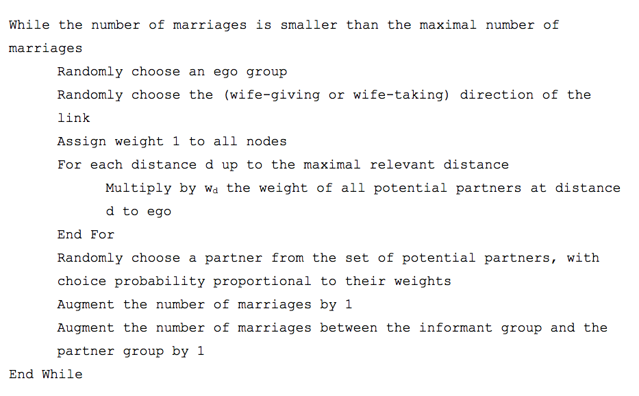
- 3.18
- The algorithm for the total virtual fieldwork process can be summarized in the following way[9]:
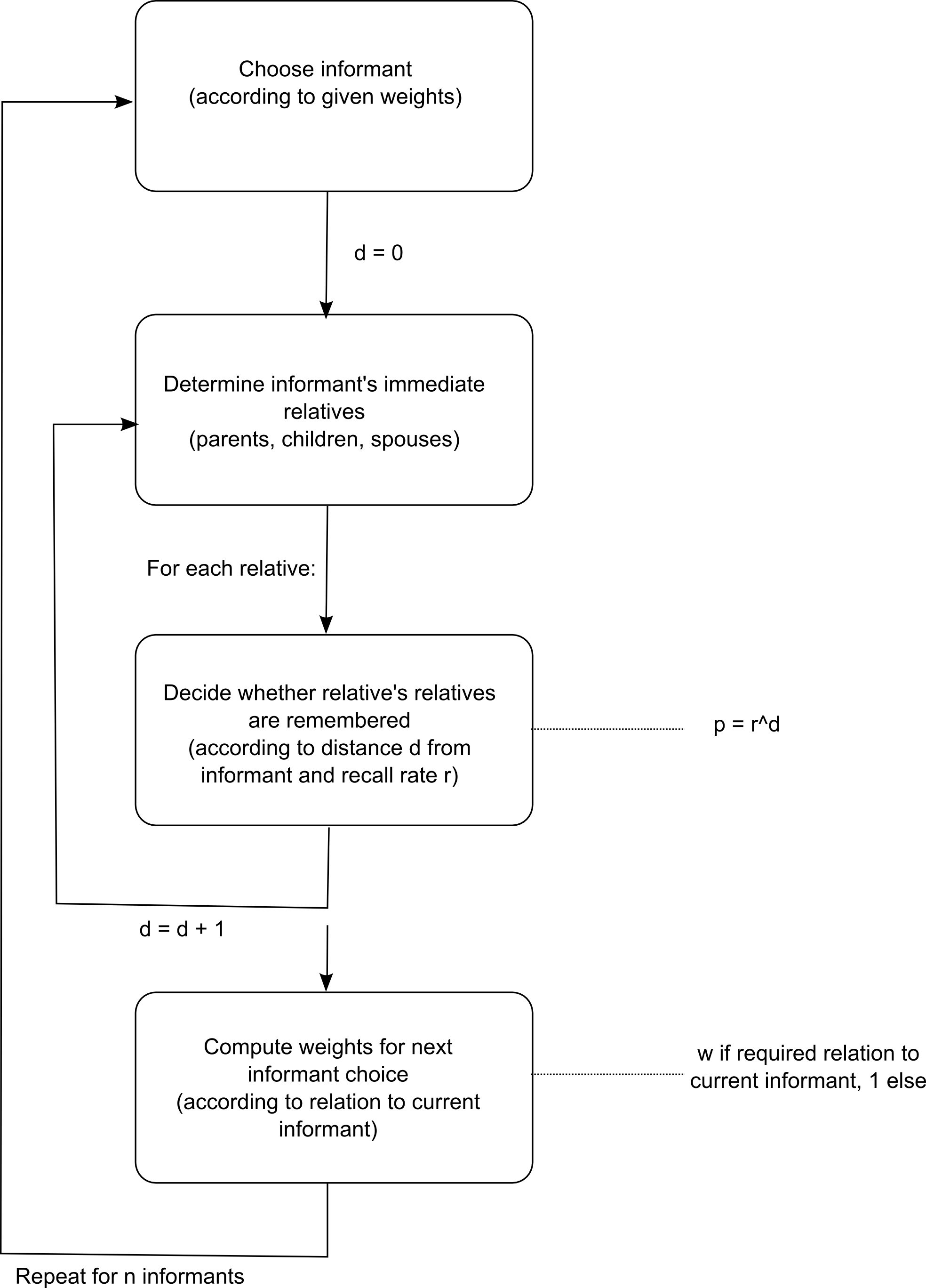
Figure 2. Virtual Fieldwork algorithm for genealogical networks 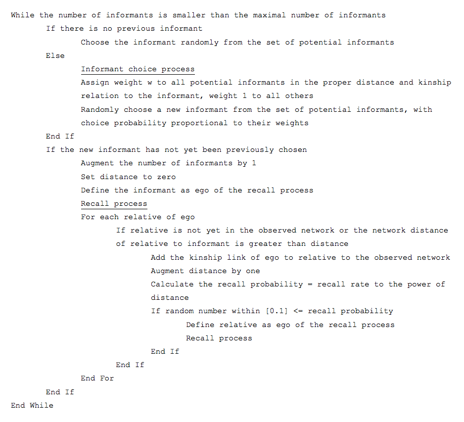
Initialization
- 3.19
- The simulation environment is initialized by choosing a network which we assume to represent the "real" social structure. This could be an empirical network we know to be unbiased and (within necessary limits) complete. As such networks are rare, we have chosen to generate the baseline networks equally by agent-based simulation. The details of the model are specified in appendix 1.
- 3.20
- We use this model to generate networks from an initial population of 1000 people who marry and procreate at a uniform rate of 2 children per couple (that is, just high enough to avoid extinction) over a period of 1000 years (in order to keep initialization effects low). People are assumed to be procreative from 15 to 50 years of age. Each year, 20% of the disposable population gets married, while at the same time 1% of marriages get divorced. Concerning matrimonial preferences, we distinguish three different scenarios:
(GN-1) random marriages
(GN-2) preference for marriage with first cousins (of whatever kind)
(GN-3) preference for marriages with first agnatic (patrilateral parallel) cousins - 3.21
- As can be seen from Table 3, the three networks have roughly the same demographic properties, but differ in the matrimonial structure. In the "neutral" network GN-1, cousin marriages make up only 0.56% of all marriages (and less than 0.2% of all cousin chains are "closed" by a marriage). In the "cousin marriage" network GN-2, the proportion of cousin marriages is 18.32%, and closure rates rise over 5%. In the "agnatic cousin marriage" network GN-3, cousin marriages account for only 5.45% of all marriages (almost all of them – 5.09% – being between agnatic cousins). As men and women are treated on a completely equal basis, the numbers of agnatic and uterine cousin relations are more or less equal (between 15.500 and 16.000), both to each other and across networks. As a consequence, agnatic and uterine closure rates are also practically equal except in network GN-3 with explicit agnatic marriage preferences, where the agnatic closure rate is 31 times higher than its uterine counterpart.
Table 3: Basic properties of the "real" genealogical networks. Individuals Marriages Cousin Marriage Closure Relations Agnatic Cognatic Uterine Total of Marr. Total Per Ind. Marriages Relations Closure Marriages Relations Closure Marriages Relations Closure GN-1 32,693 18,790 106 0.56% 0.16% 65,839 4.03 32 15,473 0.21% 45 34,639 0.13% 29 15,727 0.18% GN-2 32,700 18,955 3,472 18.32% 5.22% 66,504 4.07 855 15,622 5.47% 1,799 35,023 5.17% 833 15,859 5.25% GN-3 33,181 19,137 1,043 5.45% 1.55% 67,277 4.06 974 15,782 6.17% 44 35,327 0.12% 32 16,168 0.20% - 3.22
- We now let a virtual observer explore these networks by interviewing n = 100 informants from the lowest age cohort (between 0 and 100 years), which in our case comprises roughly 14% of the population. We let the observer's local inertia (agnatic preference) w vary from 1 (perfect mobility, where agnatic relationship presents no advantage) to 105 (extreme immobility, where subsequent informants are likely to be agnatically linked). At the same time, we let informant's recall rates r vary between a very low value of 10% (that is, a 90% memory loss at each step) and the high value of 80%. For each combination of parameters, we have effectuated 100 runs.
Results
First cousin marriages
- 3.23
- Let us first consider how agnatic cousin relations and marriages are explored for different combinations of informant memory and observer behavior (see Figure 3). Cousin relations, while initially less observable than single individuals, are explored at an increasing rate, so that the number of agnatic cousins per individual monotonicly rises as recall rates improve. Similarly, cousin marriages, being circuits of five links, are initially less observable that simple marriage links, but become explored at a higher rate, so that also the rate of agnatic cousin marriages (as a percentage of total marriages) generally increases with recall rates, at least as long as the observer's agnatic inertia is moderate.
- 3.24
- The effect of agnatic inertia shows a non-monotonic profile. As long as recall rates are low, the tendency to choose informants within a group of close agnatic relatives generally increases the number of detected agnatic first cousin relationships and, correspondingly, agnatic first cousin marriages, in the network. This is the immediate effect of the redundancy introduced by choosing informants belonging to the same agnatic sub-network as preceding informants: memory lacunae concerning agnatic kin can be more easily compensated by information from other informants than those concerning non-agnatic kin. However, this advantage of local redundancy will at some point reach its limits, and even turn to a disadvantage, as informants contribute increasingly less to the knowledge of their agnates (whom the observer knows already from preceding informants). The higher recall rates (and the less important the "assistance" from agnatic kin for "closing holes" in the kinship network), the sooner this point will be reached where a further increase in agnatic observer inertia will result in redundant information. For a highly immobile observer, increasing recall rates may even for some time lead to a diminution in the rate of observable agnatic cousin marriages.

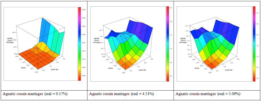
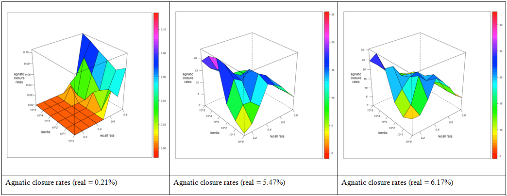
Figure 3. Agnatic first cousin relations per individual (top), agnatic first cousin (FBD) marriages as % of all marriages (middle) and agnatic closure rates (bottom) for different combinations of the observer's agnatic inertia (left depth axis) and the informants' recall rate (right depth axis). Visualization with R. Closure rates
- 3.25
- This profile characterizes both cousin relations in general and cousin marriages in particular. However, though similar in form, the exploration of "open" and matrimonially "closed" kinship chains does not proceed with the same rapidity. Cousin relations are more easily detected if they link spouses, so that cousin marriages are more rapidly explored than open cousin relations, and closure rates, while initially increasing, diminish with improving informant memory, once a sufficiently large part of cousin marriages has been explored and additionally detected cousin relationships are to an increasing extent between otherwise unrelated people. This point is reached earlier if real cousin marriages are frequent, as in networks GN-2 and GN-3. Moreover, the observer's agnatic preference, while initially augmenting closure rates, tends to diminish them from a certain point onwards. Closure rates therefore cannot serve as stable indicator for cousin marriage preferences. They may be both over- and underestimated, and evolve in a nonlinear manner both with informant memory and observer immobility.
Agnatic bias
- 3.26
- What does this mean for the relative degree of agnatic cousin relations and marriages with respect to their uterine counterparts? Although the exploration of agnatic and uterine relationships are to some extent correlated, the effect of agnatic observer bias on uterine relationships is weaker than on agnatic relationships. As a consequence, agnatic inertia increases the apparent surplus of agnatic over uterine cousin marriages, but less so as informant memory improves. However, if there is a real surplus of agnatic over uterine cousin marriages in the network, this overestimation from observer bias may just compensate the underestimation due to the insufficient detection of existing cousin marriages. Improving informant memory may therefore first result in a diminution of the surplus (as it reduces the apparent surplus of agnatic marriages introduced by the myopia of an immobile observer) but then augment it again (as the real surplus of agnatic marriages gradually comes to light) (see Figure 4, right).
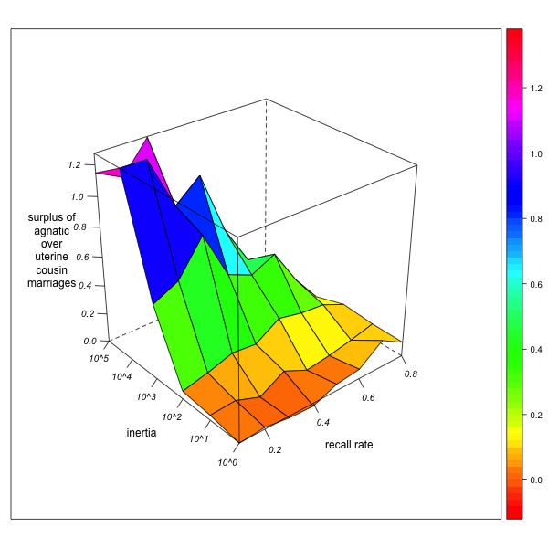
GN-2 (real surplus = 0.12) GN-3 (real surplus = 4.92) Figure 4. Surplus of agnatic over uterine first cousin marriages (as percentage of total marriages) for different combinations of local inertia (left depth axis) and recall rate (right depth axis). Visualization with R. - 3.27
- This puts the observer (and the researcher who has to deal with the data) in an uncomfortable position: a diminution of the agnatic cousin marriage surplus due to improving memory (for example by repeated field or archive research) does not by itself indicate that the formerly observed surplus was just an illusion. It only means that there is a marked agnatic observer bias – but this does not exclude that there is nevertheless a real surplus of agnatic cousin marriages, and that the observed surplus will again start to rise as memory improves further. This combination – high agnatic bias in the context of real agnatic marriage preference – probably characterizes the "Ebrei" dataset. On the one hand, we know that informants' recall rates are low and agnatic observer immobility is high (since the observer is a 17th century notary who never leaves his village, and the informants are men who are asked their parents, wives, and eventually their wife's fathers). But on the other hand, we also know (from other sources on matrimonial norms and from the inspection of patronyms) that agnatic marriages are really preferred. The genealogical data cannot, by themselves, validate or invalidate the hypothesis of agnatic marriage preferences. Reducing the dataset to an unbiased and well-explored subset (for instance, by restraining the matrimonial circuit census on spouses whose grandparents are all known) may be the only solution.
Virtual fieldwork in alliance networks
-
The model
- 5.1
- The model for alliance networks shares the basic goals and properties of the model for genealogical networks, that is, to explore the effects of observer behavior on the morphology of the observed network. In what follows, we will concentrate on the differences.
Parameters and state variables
- 5.2
- As in the preceding section, the model comprises two types of networks – the real and the observed kinship network – and two types of agents – informants and the observer. The network is now an alliance network, consisting of groups (rather than individuals), which are related by only one kind of link (marriages) – parent-child relations no longer play a role. The observed network will be recomposed from information yielded to the observer by successively chosen informant groups.
- 5.3
- The fact that informants now are groups rather than individuals, and that all links are marriage links, introduces two major simplifications. First, we shall assume that all groups show roughly the same internal generational profile, so that any group may be chosen with the same probability as an interview partner. We thus do not need to define from the outset a subset of potential informant groups as in the case of genealogical networks. Second, we assume that groups have perfect memory of their members' marriages (one group member completing the lacunae of the other), so that memory constraints play no role.
- 5.4
- As a consequence, asking each informant group to reveal the complete network of allies would hardly be possible without considerably reducing the number of groups to be visited. We thus let the length of the interview depend on the observer's choice, or, what amounts to the same thing, we allow the chosen informant group to be identical to the actual group, each group revealing a single marriage link at a time step t. Accordingly, the duration of the virtual fieldwork process is no longer limited by a given number of informants, but by a given number of observed links.
- 5.5
- Again, the observer choses his or her informant group according to its distance to the previous informant group. As there are no parent-child links in alliance networks, distance is measured simply as the number of marriage links. Observer inertia can thus be modeled as a preference for staying with one and the same informant group, that is, for a distance of zero between the next and the previous informant group. We may, however, also model a different type of observer behavior, characterized by a preference for a distance of 1. This behavior corresponds to a strategy of "snowballing", that is, of choosing the next informant group among the revealed direct allies of the last informant group. Note that, since this sort of "closeness" is considered as a social rather than a spatial constraint, we have to define it in terms of revealed rather than of total marriage links. In a snowballing model, the observed network feeds back into observer behavior, which was not the case in the model for genealogical networks.
- 5.6
- To sum up, the alliance network model is characterized by the following (constant) parameters:
- The real network (number of groups, number of links, incidence of links and groups)
- The observer's informant choice preferences (inertia w1 and snowballing w2)
- The number of links to be observed n
- The actual informant group at time t
- The marriage link and the partner group revealed by the informant group at time t
- The set of potential informant groups (whose marriage links have not yet been totally revealed)
- The observed network at time t (which is composed of all groups and links revealed from 1 to t)
Process overview
- 5.7
- At the beginning, the observed network consists only of a single informant group chosen at random. The virtual fieldwork process is modeled as a sequence of choices of (not necessarily distinct) informant groups. At each time step, the observer asks the (members of the) group to reveal one additional marriage link that has not already been documented[10]. While the observer may thus ask the same group several questions, he or she will not count the same marriage link twice, but continue his fieldwork process until the desired number of links has been attained. Whether or not a marriage link has been revealed, a new informant group (which may be identical to the old) is chosen at each time step. The observer may thus potentially stay with one and the same group until all marriage links of this group have been explored.
Marriage link revelation process
- 5.8
- Groups are no longer endowed with a recall function. They chose the revealed marriage link at random from among the marriages that have not yet been revealed. Moreover, they will also reveal to the observer the fact that there are no longer any unrevealed marriages (so that he or she can avoid visiting them in the future).
Informant choice process
- 5.9
- As in the case of genealogical networks, the observer's choice incorporates a weight function assigning a weight wd to groups at a distance of d from the actual informant group (see above). We consider only preferences for d = 0 and d = 1 (for all higher distances, the weight is set equal to 1). Groups whose links have already been totally explored are assigned weight 0 and thus will no longer be visited. While the set of potential informants, contrary to genealogical networks, is not limited at the outset, it thus becomes gradually limited as the virtual fieldwork process advances[11].
Process summary
- 5.10
- The algorithm for the total virtual fieldwork process can be summarized in the following way [12]:
Figure 5. Virtual Fieldwork algorithm for alliance networks 
Initialization
- 5.11
- As in the previous section, the model will be initialized by choosing a baseline network which is itself the result of a simulation. Simulation of alliance networks is simpler than that of genealogical networks, as they can be generated solely by a series of matrimonial choices, where matrimonial preferences and avoidances are modeled as a function of distance. Thus, in strongly endogamous societies there is a preference for marrying people in the same group, in societies with a preference for marriage relinkings there will be a tendency to redoubling the links with neighbors at distance one, and so on. As a consequence, we can generate alliance networks through a process quite similar to the virtual fieldwork process, the only difference being that we let groups choose their marriage partners rather than let the observer choose his or her interview partners. The model is presented in appendix 2. Note that the uniform probability for each group to be chosen as the first marriage partner (who then chooses the second partner group) results in a homogenous network structure. This homogeneity feature is crucial for the results.
- 5.12
- We generate alliance networks composed by m = 150 nodes and n = 6000 matrimonial connections. Concerning matrimonial preferences, we distinguish four prototypical kinship scenarios (we limit our analysis to d<3, fixing wd>2=1):
(AN-1) random marriages (w0=1, w1=1, w2=1)
The morphological properties of the networks thus generated are represented in Table 4.
(AN-2) preference for endogamous marriages (w0=100, w1=1, w2=1)
(AN-3) preference for marriage relinking with allies (w0=1, w1=105, w2=1)
(AN-4) preference for indirect marriage relinking with allies' allies (w0=1, w1=1, w2=105)Table 4: Basic properties of the "real" alliance networks Max.
Marr./GroupMax.
Marr./PairComponents Loops Dual circuits Triangles Absolute Normalized Absolute Normalized Absolute Normalized AN-1 104 4 1 47 0.0078333 1,683 0.0000935 72,764 0.00000034 AN-2 103 32 1 2412 0.492 551 0.0000306 15,899 0.00000006 AN-3 188 53 39 1 0.0000166 179,091 0.0099495 19,410 0.00000010 AN-4 104 29 21 1 0.0000166 41,028 0.0022793 1,380,870 0.00000639 - 5.13
- The logic of network construction manifests itself in a straightforward manner in the frequencies of the corresponding morphological features: endogamy preference leads to a high number of loops, direct relinking preference to a high number of dual circuits, indirect relinking preference to a high number of triangles. All three kinds of preferences lead to an increased concentration of marriages between pairs of groups and thus raise the maximal number of marriages by pair.
- 5.14
- Relinking also leads to a segmentation of the network: while the random network constitutes one single giant component, the triangular relinking of AN-4 leads to the emergence of several clusters of groups closely linked with each other by repeated marriages, and thus showing a sort of higher-level "endogamous" behavior. The dual relinking of AN-3, while hindering the emergence of triangles, favors the emergence of dyads or open triads and a still higher degree of segmentation into mutually disconnected alliance clusters.
- 5.15
- We now proceed to the virtual exploration of these networks, considering different values of observer inertia and snowballing attitudes (from a strong aversion value of 10-5 to a high preference value of 105). We have run experiments for exploration rates of 10%, 50% and 75%. The following diagrams draw on the case of a 10% (600 links) exploration. In each case, we consider the normalized numbers of the configurations in question (loops, dual circuits and triangles) as a ratio of observed to real values (that is, as an indicator of over- or underestimation).
Results
Endogamy (Number of Loops)

AN-1 (real number of loops = 46) AN-2 (real number of loops = 2412) Figure 6. Effect of local inertia (right depth axis) and snowballing (left depth axis) on the over- or underestimation of normalized loop frequencies (endogamy rates).Visualization with R. - 5.16
- As can be seen from figure 6, endogamy rates are generally correctly estimated. Only if the observer is extremely immobile (combining a high local inertia with an aversion against snowballing), the fact that endogamous marriages can only be observed from "within" a group (whereas exogamous marriages can also be observed from any partner group) may lead to an underestimation of the global endogamy rate, which diminishes as network exploration advances.
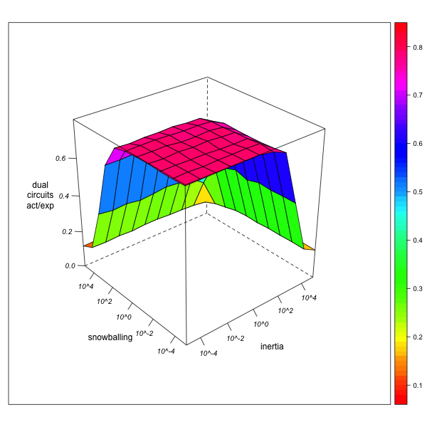
Dual Circuits
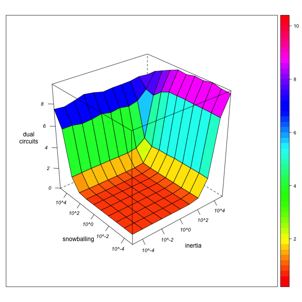
AN-1 (real number of circuits = 1683) AN-3 (real number of circuits = 179091) Figure 7. Effect of local inertia (right depth axis) and snowballing (left depth axis) on the over- or underestimation of normalized dual circuit frequencies (relinking rates). Visualization with R. - 5.17
- A similar effect of observer "myopia" can be stated with respect to the number of dual circuits (see figure 7): if the observer is immobile (combining high inertia with an aversion against snowballing), node-pairs that have not been explored appear as node-pairs that are not linked by any marriage, thus creating the illusion of an unequal distribution of marriages across pairs of nodes. As a consequence, the normalized number of circuits is overestimated[13]. Again, the degree of this overestimation diminishes as network exploration augments.
- 5.18
- The effect of snowballing is more ambiguous. Snowballing can be considered from two aspects: it is "extroverted" at a micro-level (as it pushes the observer to move between groups) but "introverted" at a macro-level (as it keeps the observer inside a cluster of groups linked with each other). If local inertia is high, snowballing acts as a countervailing tendency to break away from the precedent informant group and thus attenuates the distortive effect of inertia on observed circuit numbers. If, on the other hand, local inertia is low, snowballing tends to reduce the observer's mobility, all the more if the underlying network is highly clustered (as in the case of AN-3) and snowballing thus amounts to a form of macro-inertia (the observer will be stuck within the same cluster of closely interconnected groups). In the case of AN-1, where no such cluster structures are present, this effect is not observed. In other words, the more circuits there are in the network, the more an observer following a snowballing strategy will tend to overestimate their number even further.
Triangles
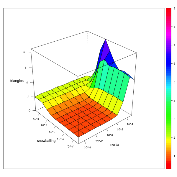
AN-1 (real number of triangles = 72764) AN-4 (real number of triangles = 1380870) Figure 8. Effect of local inertia (right depth axis) and snowballing (left depth axis) on the over- or underestimation of normalized triangle frequencies (rates of indirect relinking). Visualization with R. - 5.19
- This self-reinforcing effect can also be observed for triangles (figure 8). In the "neutral" network AN-1, the effect of snowballing will be ambiguous: it is necessary for the reconstruction of triangular marriages (a totally immobile observer can see no triangles, but only star-like configurations), but at the same time, it mitigates the tendency for triangular structures to emerge from the marriages with one and the same group. If triangles are very frequent, however, a snowballing observer will remain imprisoned within them, and neglect the dyadic or isolated endogamic configurations elsewhere in the network. Again, then, the overestimation of triangles in the observed network may be a consequence of their actual presence in the real network.
Expected marriage indicators
- 5.20
- As we have indicated above, matrimonial strength (that is, the numbers of marriages concluded by each group) can be used to calculate the numbers of marriage configurations that would result if each group chose its marriage partners at random (Roth et al. 2013). The ratio of observed to expected values can then serve as an indicator of the non-random character of matrimonial patterns in alliance networks. However, the "non-random" causes of these configurations are not necessarily to be found in agent behavior – they may also be due to observer behavior. It is therefore crucial to assess the relative impact which observer behavior has on the observed and on the expected numbers of matrimonial configurations.
- 5.21
- Let us concentrate on the case of dual circuits (relinking marriages). As can be seen from Figure 9, the ratio of their observed to their expected numbers in the data collected by the virtual observer is always underestimated, quite independently of observer behavior. These results also hold, on a lesser scale, for higher degrees of network exploration, where high observer mobility (avoiding both local inertia and snowballing) increasingly leads to correct estimation of dual circuit numbers.
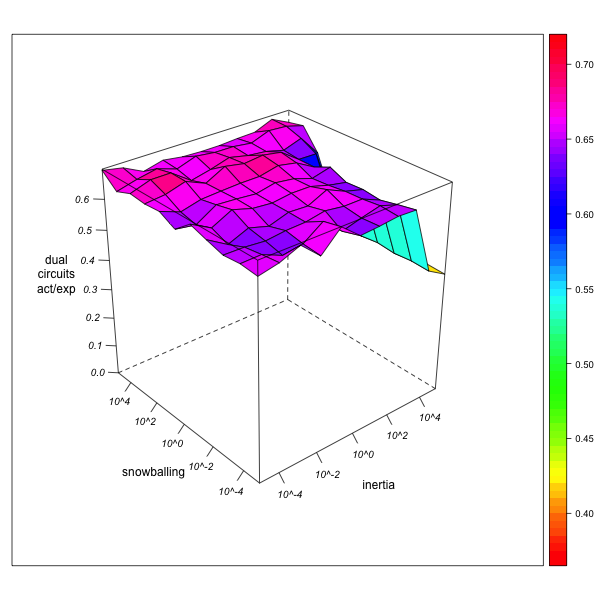
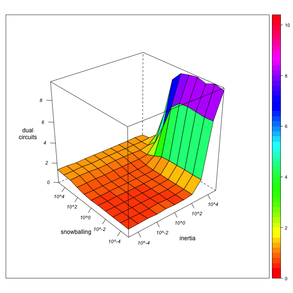
AN-1 (real divergence actual/expected = 1.1) AN-3 (real divergence actual/expected = 92.87) Figure 9. Effect of local inertia (right depth axis) and snowballing (left depth axis) on the over- or underestimation of the divergence of actual from expected circuit frequencies (relinking rates). Visualization with R. - 5.22
- In other words, while observer inertia and snowballing may both tend to overestimate the real number of dual circuits, they also, and even more so, tend to overestimate the concentration of matrimonial strengths from which expected numbers of dual circuits are calculated. As a result, the divergence of observed from expected numbers is never higher for the observer than it would be in the case of complete network exploration.
- 5.23
- These findings have an important practical implication: observed numbers of endogamous or relinking marriages in excess of their expected numbers, that is, high enough to counterbalance the effect of observer bias, appear to be a strong sign of real underlying non-random mechanisms (such as social norms and institutions). For the Ebrei network, this means that the endogamic tendency of agnatic groups, showing an endogamy rate much higher than expected, is likely to be a real property of the network.
Conclusion
- 6.1
- As our simulation experiments show, the morphological indicators of kinship and alliance networks most likely to be interpreted in terms of social structure – matrimonial circuit numbers – are never the sole product of agent behavior. Observer behavior, if only stemming from inevitably limited mobility, introduces a bias in the numbers not only of actual circuits, but also of potential circuits (open kinship chains in genealogical networks) and of expected circuits (as calculated from matrimonial strengths in alliance networks).
- 6.2
- In the case of genealogical networks, the effect of observer inertia on actual and potential matrimonial circuits is nonlinear and may affect their ratio both in a positive and in a negative way, depending on overall genealogical memory. Neither absolute circuit frequencies nor closure rates (percentages of kinship chains that link spouses) can serve as an unbiased indicator of matrimonial preferences.
- 6.3
- Concerning alliance networks, the more immobile the observer, the more will he tend to underestimate endogamy and overestimate marriage relinkings as well as the concentration of matrimonial strengths. However, the case of alliance networks is somewhat more favorable, as observer bias tends to lower the ratio of observed over expected circuits. A high and positive ratio may therefore serve as a valid measure for observer-independent non-random causes underlying the network morphology.
- 6.4
- We hope to have demonstrated how sensitive the supposed indicators of matrimonial behavior are to the mobility constraints which even the most meticulous researcher necessarily faces when collecting kinship and marriage data. Any reasonable interpretation of the collected data rests crucially on a clear idea of the conditions and the methodology used during fieldwork research. The difference between "data" and "metadata" here becomes increasingly blurred. Information on informants and the way they are related both with each other and with the reported members of the genealogical network is as essential for the reconstruction process as information on the network itself. Without this complementary information, genealogical datasets and matrimonial censuses cannot be used to validate or invalidate the informants' or the ethnographers' claims concerning prevalent matrimonial practices in a given society. The interest in empirical kinship and marriage data stems from the conviction that what people say should be checked by observing what they actually do. However, for this principle to be viable, it has to be applied first and foremost to the observer him- or herself.
Appendix: Generation of the Baseline Networks
-
Appendix 1: Generating genealogical networks
- 7.1
- The algorithm we use to generate genealogical networks is a variant of a model developed by Telmo Menezes (Menezes et al., s.d.), which combines both global (growth, marriage and divorce rates) and individual (age and kinship) state variables and parameters[14]. Its parameters are:
- The size of the initial population
- The number of years
- The maximal and minimal age for having children
- The marriage rate (as a fraction of the number of potential couples)
- The fertility rate (as a fraction of the number of adults divided by two times the number of fertile years)
- The divorce rate (as a fraction of fertile families)
- The type and strength of matrimonial preferences
- The numbers of marriages, births and divorces occurring at time t
- The children, adults, marriageable men and women, and fertile families at time t
- The kinship network at time t (composed of all individuals and families created up to time t)

Appendix 2: Generating alliance networks
- 7.2
- The model for generating alliance networks builds on the same principles as the Virtual Fieldwork model, the difference being that we let groups choose their partners, while in the Virtual Fieldwork model we let an observer choose his or her informants.
- 7.3
- The model is characterized by the following (constant) parameters:
- The number of groups m
- The number of links n
- The groups' preferences wd for choosing partners at a distance d of 0, 1 and 2 (endogamy, direct relinking, indirect relinking)
- The ego group at time t
- The partner group chosen by the ego group at time t
- The network at time t (which is composed of all groups, as well as of all links established from 1 to t)
- 7.4
- At the beginning of the simulation all the m nodes (groups) are present but mutually unrelated. At each time step a group is randomly selected with uniform probability. This group will assign a weight wi to all the groups of the network (including the ego group itself) according to their distances from it. Again, wd = 0 represents a prohibition toward establishing marriage alliances with groups at distance d, wd < 1 avoidance, wd = 1 neutrality and wd > 1 preference. The same group may be related to the ego group by paths of different length and thus receive more than one weight (for instance, a group may be avoided as an ally's ally but at the same time be preferred as an ally). However, we do not treat ego as its own ally, ally's ally, and so on, so that endogamic behavior cannot result as a side effect of relinking behavior of any kind. The total weight of a group is the product of the weight factors:
 . After all the weights have been assigned, a link is created with a node j (that can be also the origin node) selected with probability
  . This procedure is repeated until all the n links are assigned.
- 7.5
- The process thus boils down to a sequence of partner choice processes by randomly chosen groups[16]:
Acknowledgements
- This work has been partially supported by the French National Agency of Research (ANR) through grant “SIMPA” ANR-09-SYSC-013-02. The paper has benefited from regular interactions with the members of the research group TIP (Traitement Informatique de la Parenté, http://www.kintip.net). We are particularly grateful to Camille Roth, Telmo Menezes and Michael Gasperoni for their many valuable comments on earlier versions of this article, as well as to Anne Garcia-Fernandez for her assistance with the diagrams. All errors, of course, are ours.
Notes
-
1 Kinship networks are here represented as "Ore-graphs". This representation (rather than P-graphs, where nodes represent unions) is reasonable for modeling the data collection process as a series of interviews with individuals (rather than households).
2 Alternatively, they can be represented as oriented valued graphs, where arc values correspond to the number of marriages.
3 https://www.kinsources.net/kidarep/dataset-94-ebrei.xhtml.
4 More formally, the matrimonial in- and out-strength of node i is defined as ki = ∑j xij and as k'i = ∑j xji. It follows straightforwardly that ∑i ki = ∑i k'i = n.
5 See in particular the classes org.tip.puck.net.random.RandomNetExplorer for the genealogical network model, and org.tip.puck.graphs.random.RandomGraphMaker for the alliance network model. The software allows one to generate both one-shot simulations and statistics of multiple-run simulations with variation of chosen parameters.
6 In our framework a time-step is an algorithmic step represented by the single action of the agents, not a step in real physical time.
7 This is an extension of Ebbinghaus' ([1885] 1913) law for memory loss as a function of temporal distance to genealogical distance. The particular form of the genealogical memory loss function is not, however, important for the present study, as long as it produces ever sparser genealogical networks as memory decreases.
8 In practice, there may be divergences between the memorized subnetworks of different informants, which necessitate a choice by the observer. These divergences usually arise from memory errors rather than from wilful falsification and may thus be assimilated to memory lacunae. In our model, the absence of information from a given informant can be interpreted as including doubtful or contradictory information not taken into account by a (well advised) observer. We do not, however, model the observer's choice function and the possible biases arising from it.
9 The pseudocode is implemented by the method org.tip.puck.net.random.RandomNetExplorer# createRandomNetByObserverSimulation of the software Puck 2.0
10 The model implemented in the software Puck allows the user to specify the observer's propensity to ask for a wife-giving or a wife-taking link. In the model used for this paper, we have set this propensity equal to neutrality (0.5).
11 This is a mere technical device without any impact on the results – it simply renders the model faster.
12 The pseudocode is implemented by the method org.tip.puck.graph.random.RandomGraphMaker# createRandomGraphByObserverSimulation of the software Puck 2.0
13 This generally only holds for homogenous networks, where circuits are equally distributed. If circuits are concentrated in some regions of the network, observer myopia may well lead to their underestimation.
14 Menezes' original model treats marriages and births as one and the same kind of event. Despite its obvious advantage of reducing the number of parameters, it has the disadvantage that it leads to a systematic correlation of cousin relations and cousin marriage numbers. We have therefore opted for a more "classical'" variant, but remain indebted to Menezes' original work. Both models are implemented in the software Puck 2.0.
15 The pseudocode is implemented by the method org.tip.puck.net.random.RandomNetMaker# createRandomNet of the software Puck 2.0
16 The pseudocode is implemented by the method org.tip.puck.graphs.random.RandomGraphMaker# createRandomGraphByAgentSimulation of the software Puck 2.0
References
-
BARRY, L. (2004). Historique et Spécificités Techniques du Programme Genos. Ecole " Collecte et traitement des données de parenté". http://llacan.vjf.cnrs.fr/SousSites/EcoleDonnees/extras/Genos.pdf
BARRY, L., & Gasperoni, M. (2008). L'oubli des origines. Amnésie et information généalogiques en histoire et en ethnologie. Annales de Démographie Historique, 116, 53–104.
EBBINGHAUS, H. ([1885] 1913). Memory: A contribution to experimental psychology. H. A. Ruger & C. E. Bussenius, Transl. New York, N.Y.: Columbia University, Teachers college. [doi:10.1037/10011-000]
FISCHER, M. D. (1986). Expert Systems and Anthropological Analysis. Bulletin of Information in Computing and Anthropology, 4, 1–4.
FISCHER, M. D. (1994). Modeling complexity and change: Social knowledge and social process. In J. Hann (Ed.), When History Accelerates. Essays on Rapid Social Change, Complexity and Creativity (pp. 75–94). London: The Athlone Press.
FISCHER, M. D. (2006). The Ideation and Instantiation of Arranging Marriage within an Urban Community in Pakistan, 1982–2000. Contemporary South Asia, 15(3), 325–339. [doi:10.1080/09584930601098067]
GARGIULO, F. & Roth C. (s.d.). Inertial exploration of weighted networks. Unpublished working paper, SIMPA project.
GASPERONI, M. (2011). La communauté juive de la République de Saint-Marin, XVIe-XVIIe siècles. Paris: Editions Publibook Université.
GASPERONI, M. (2013). De la parenté à l'époque moderne : systèmes, réseaux et pratiques. Juifs et Chrétiens en Italie centrale. Unpublished doctoral thesis: École des hautes études en sciences sociales, Paris.
GELLER, A., Harrison, J.F., Revelle, M. (2011). Growing Social Structure: An Empirical Multiagent Excursion into Kinship in Rural North-West Frontier Province, Structure and Dynamics, 5(1), 3, http://www.escholarship.org/uc/item/4ww6x6gm.
GILBERT, J.P. & Hammel, E. (1966). Computer simulation and analysis of problems in kinship and social structure. American Anthropologist, 68, 71–93. [doi:10.1525/aa.1966.68.1.02a00070]
HAMBERGER, K. (2011). Matrimonial circuits in kinship networks: calculation, enumeration and census. Social Networks, 33, 113–128. http://www.sciencedirect.com/science/article/pii/S0378873310000511 [doi:10.1016/j.socnet.2010.10.002]
HAMBERGER, K., Grange, C., Houseman, M. & Momon, C. (2014). Scanning for Patterns of Relationship. Analyzing Kinship and Marriage Networks with Puck 2.0. History of the Family. http://www.tandfonline.com/doi/full/10.1080/1081602X.2014.892436#.U5sFGHZFsuc.
HAMBERGER, K., Houseman, M. & Grange, C. (2009). La parenté radiographiée: Un nouveau logiciel pour l'analyse des réseaux matrimoniaux. L'Homme, 189, 107–137.
HAMBERGER, K., Houseman, M. & White, D. (2011). Kinship network analysis. In P. Carrington & J. Scott (Eds.), The Sage Handbook of Social Network Analysis (pp. 533–549). London: Sage.
HEYMANN, F., (1994). L'obligation de mariage dans un degré rapproché. Modèles bibliques et halakhiques. In P. Bonte (Ed.), Epouser au plus proche. Inceste, prohibitions et stratégies matrimoniales autour de la Méditerranée (pp. 97–111). Paris: Éditions de l'EHESS.
KUNSTADTER, P., Buhler, R., Stephan, F. & Westoff, C. (1963). Demographic variability and preferential marriage patterns. American Journal of Physical Anthropology, 2, 511–519. [doi:10.1002/ajpa.1330210408]
MENEZES, T., Gargiulo, F., Roth, C. & Hamberger, K. (s.d.), New Simulation Techniques in Kinship Network Analysis. Submitted to Structure and Dynamics.
READ, D. (1998). Kinship based demographic simulation of societal processes. Journal of Artificial Societies and Social Simulation, 1(1), 1 <https://www.jasss.org/1/1/1.html>.
ROTH, C., Gargiulo, F., Bringe, A. & Hamberger, K. (2013). Random Alliance Networks. Social Networks 35 (3), 394–405, <http://www.sciencedirect.com/science/article/pii/S0378873313000427>. [doi:10.1016/j.socnet.2013.04.006]
SMALL, C. A. (2000). The political impact of marriage in a virtual Polynesian society, In T. A. Kohler & G. J. Gumerman (Eds.), Dynamics in Human and Primate Societies: Agent-Based Modeling of Social and Spatial Processes (pp. 207–224). New York: Oxford Unviersity Press.
WHITE, D. (1999). Controlled simulation of marriage systems. Journal of Artificial Societies and Social Simulation, 2(3), 5 <https://www.jasss.org/2/3/5.html>.
WHITE, D. & Jorion, P. (1992). Representing and analyzing kinship: a new approach. Current Anthropology, 33, 454–462. [doi:10.1086/204097]
WHITE, D. R., Batagelj, V. & Mrvar, A. (1999). Analyzing large kinship and marriage networks with Pgraph and Pajek. Social Science Computer Review, 17 (3), 245–74. [doi:10.1177/089443939901700302]