
 Abstract
- We develop an agent-based model that captures the dynamic processes related to moving from an educational system in which students are automatically assigned to a neighborhood school to one that gives households more choice among existing and newly formed public schools. Analysis of our model reveals the importance of considering the timing of the entrance of new schools into the system in addition to their quantity and quality. Our model further reveals a range of conditions where the more households emphasize school achievement relative to geographic proximity in their school choice decision, the lower the mean achievement of the district – a paradoxical mismatch between micro- and macro-levels of behavior. We use data from Chicago Public Schools to initialize the model.
- Keywords:
- Public Policy, Education, School Choice
Introduction
- 1.1
- Much controversy surrounds education reforms that move away from catchment area systems, where students are required to attend an assigned geographically proximate school, towards choice-based systems, where households have more choice and control over the schools their children attend. Proponents of choice-based reforms claim that increased choice provides both access to better schooling for disadvantaged populations as well as the incentives necessary for school reform (Chubb & Moe 1990). Opponents of school choice, by contrast, claim that choice-based programs will not bring about the desired improvements in schools but instead only drain resources from troubled schools that can least afford to lose them (Fiske & Ladd 2000). As might be expected, the debate hinges in large part on what one believes about household behavior when given a choice of schools. For example, the more one believes that households do not have the information, resources, and preferences to move to better schools, the more likely one is to believe that a choice system would not lead to desirable district-level outcomes. The purpose of this paper is to examine this important relationship between household-level decision-making and district-level outcomes in school choice systems.
- 1.2
- To this end, we developed an agent-based model (Wilensky & Rand 2013; Gilbert 2008) of a school district's transition from a catchment area system to a common form of school choice where households, while able to choose among public schools in the district, do not receive vouchers to go outside of the public system. The agents in our model are schools and students.[1] Schools vary in quality and building capacity, with new schools that enter the system imitating the top performers. Students vary in ability and background. Students rank schools by using a preference function based on the mean achievement and geographic proximity of a school. Their academic achievement results from a combination of individual traits and the "value-added" parameter of the school they attended. We use data from Chicago Public Schools to initialize the model in a plausible manner.
- 1.3
- The model demonstrates the importance of considering the timing of the entrance of new schools into the system in addition to their quantity and quality. Analysis of the model further reveals a paradoxical mismatch between micro- and macro-levels of behavior, as increased emphasis on school achievement at the household-level often does not lead to increased district-level achievement. The intuition is as follows: A high emphasis on school achievement results in new schools entering the system earlier in the life of the program. Since the primary improvement mechanism of the system involves new entrants imitating the top performers, such front-loaded entry of new schools forgoes the benefit that comes from late entrants who have an opportunity to imitate a population of higher quality schools.
- 1.4
- The paper proceeds in four main sections. The first section introduces existing empirical and computational work and literature on school choice. The second section presents a highly stylized agent-based model of the transition from a catchment area to public choice system to illustrate our approach, and further motivates the importance of understanding the relationship between student behavior and district-level outcomes. The third section develops and presents results from a more detailed model of the transition to school choice, using data from Chicago Public School's school choice program to initialize parameters. The final section discusses limitations and outlines areas of future work.
School choice
- 2.1
- School choice comes in a variety of forms. One distinguishing feature is the inclusion of private schools. For example, in countries such as Chile, Sweden, and Denmark, public funds can be utilized to attend privately operated schools; while in other countries, such as the United Kingdom and New Zealand, have implemented "open enrollment" programs where households can only choose among other public schools; yet in others such as the United States and Canada, the inclusion of private schools varies by locality. Another distinguishing feature is the creation of new schools, often with a specialized theme or mission, and sometimes with selective admissions criteria for students. In the United States, for example, an early form of choice involved the development of specialized and publicly operated "magnet" to which students could apply to attend instead of their catchment area school. More recently, states and school districts have allowed professional school operators and interested community members to apply for "charters" to create and run schools that receive public funding on a per-pupil basis. Oversubscription at publicly funded schools without selective criteria is often handled by a randomized lottery.
- 2.2
- Empirical research on the causal effect of these various forms of choice consists of two broad streams. One line of research investigates whether the students who attend choice schools (e.g., private schools, public magnet schools, charter schools) are better off than those who do not. Observational studies using a variety of approaches to account for selection bias have resulted in disputed findings, with some finding better educational outcomes for students who attend magnet (Gamoran 1996) or Catholic schools (Bryk et al. 1993; Coleman et al. 1982; Evans & Schwab 1995; Morgan 2001); others finding little to no effect on academic achievement (Alexander & Pallas 1983; Goldhaber 1996; Neal 1997); and still others raising serious concerns about the approach used to deal with selection bias (Altonji et al. 2002). Moreover, field studies taking advantage of the lotteries put in place to deal with oversubscription to choice programs have not yielded conclusive evidence on the "treatment effect" for choosers. Randomized field trials of pilot voucher programs in Milwaukee (Greene et al. 1999; Rouse 1998; Witte et al. 1995), New York City, Dayton, and Washington, D.C. (Howell et al. 2002), have yielded effect sizes ranging from small to modest, with debates around methodological issues pertaining to selective attrition in Milwaukee (Witte 1997) and subgroup definition in New York City (Krueger & Zhu 2004). Cullen et al. (2006) find that lottery winners in Chicago's public choice program experience improvements in nontraditional outcomes such as reduction in disciplinary incidents, but not in more traditional measures such as test scores and drop-out rates.
- 2.3
- Of course, even if one could establish a clear causal relationship between attending choice schools and academic performance, such findings would have to come with the caveat that they do not evaluate the systemic effect of choice programs. Improvement could arise from a number of mechanisms that go beyond students' sorting themselves into better schools, particularly through the competition and new investment induced by household choice (e.g., Hoxby 2003). Indeed, embedded in the logic of school choice reform is the following dynamic causal story: More choice leads to the movement of students. Schools losing students feel pressure to change in order to attract and keep students, which in turn creates pressure for all schools to change. Choice also creates the opportunity for new schools to enter the market, providing students with a wider range of options, and further increasing the competitive pressure on existing schools. Bad or undesirable schools improve or close; good or desirable ones survive; and new, stable levels of enrollments, school types, and student achievement are reached. If the subsequent resorting of students does not lead to clusters of low achieving students, or if the spillover effects of that clustering are not large, the mean level of student achievement will be higher than before.
- 2.4
- Relatedly, a second line of empirical school choice research attempts to identify a causal effect on system-level performance by exploiting variation in competition across metropolitan areas. These studies typically investigate the relationship between indicators of competition levels such as market concentration ratios or private school enrollments, and academic outcomes such as test scores and graduation rates. Belfield & Levin (2002) review this literature and find results ranging from no statistical significance to modestly sized associations. The potentially endogenous nature of the competition measures used in this work, however, make pinpointing the causal effect difficult, and have led to substantial controversy over the techniques used to ameliorate such concerns (e.g., Hoxby 2005; Rothstein 2005).
- 2.5
- A third area of work regarding school choice recognizes that even with greater confidence in the empirical association between system-level outcomes and competition measures, we still need to know more about the systemic implications of school choice in order to fully evaluate the impact of such programs. Computational general equilibrium (CGE) models of school finance (Epple & Romano 1998; Nechyba 2000; Fernandez & Rogerson 2003; Ferreyra 2007) capture the idea that changes in school financing through school choice programs can impact the larger economic environment (through the housing market, for example), and vice versa. Such models have been employed to examine interactions between education choice and residential mobility, as well as understanding the implication of various designs of systems that allow government-issued vouchers to be used in private schools (for review, see Nechyba 2003).
- 2.6
- While not in the same modeling tradition, our study can be viewed as a complement to CGE work in two respects. First, CGE models typically make assumptions about school and student behavior required to ensure an equilibrium, calibrate parameters of that model to values consistent with aggregate data, and then ask questions about how different school financing systems would impact the equilibrium characteristics of that system given the calibration. In our agent-based model, we initialize students and schools with micro-level data, and then ask the complementary question of how educational outcomes for a given choice program might vary under different assumptions about how students choose schools. Second, in addition to examining the systems' long-term outcomes, our approach also closely examines the paths to those outcomes. From a policy perspective, the paths are equally important both because key outcomes may reach unacceptable levels en route to equilibrium, as well as because policymakers may want to implement adaptive policies that conscientiously change over time.
- 2.7
- Our research could also be deemed a more general contribution to the literature on education and agent-based modeling. The most fully developed work in this area has focused on how agent- based modeling can be used inside the classroom to improve student learning (Stonedahl et al. 2011; Blikstein & Wilensky 2010; Jones & Laughlin 2009; Sengupta & Wilensky 2009; Wilkerson 2009; Epstein 2006; Wilensky & Reisman 2006; Colella et al. 2001; Wilensky & Resnick 1999), with a special emphasis on the "restructuration" of knowledge enabled by ABM (Wilensky & Papert 2010). A much smaller body of literature uses ABM and the complex systems perspective to reconceptualize and investigate educational systems themselves (Montes 2012; Maroulis et al. 2010; Lemke & Sabelli 2008; Henrickson 2002), as well as a tool for educational planning (Harland & Heppenstall 2012). Our paper contributes to this literature by operationalizing many of the implications of a complex systems perspective in the context of choice-based reforms in the United States.
Model I: An illustrative example
- 3.1
- In this section, we present a highly stylized agent-based model of a school district with two sets of agents – schools and students. The district is comprised of nine neighborhoods, each containing one school, and students residing in a particular neighborhood can only attend their neighborhood school. For illustrative purposes, Model I leaves out complicating factors such as capacity constraints and heterogeneity in student decision-making and simply asks: What if we could change the world in a way where, from this point forward, all new students were able to attend the school with the highest mean achievement?[2]
Model Description
- 3.2
- The simulation takes place on a grid of 18 × 18 sites that represent the geography of the school district. The district is equally divided into nine neighborhoods with clear boundaries, as shown in Figure 1. One school is set in each of the nine neighborhoods of the district, and each school is comprised of four grades, with an approximately equal number of students in each grade. The district contains 150 total students whose location is determined by a random draw from a uniform distribution of all locations on the 18 × 18 grid. Each neighborhood differs in its mean level of socioeconomic status (SES). Model I reflects this difference in neighborhoods by initializing students that reside in each neighborhood with different levels of achievement. The students residing in Neighborhood 9 have the highest mean achievement, the students in Neighborhood 1, the lowest, with a constant decrease in mean achievement between Neighborhoods 9 and 1. Achievement across students is distributed normally within each neighborhood, allowing for some overlap in distributions between neighborhoods.
- 3.3
- In the initial state of the model, all students are required to attend their respective neighborhood schools. When given the opportunity to choose, students have perfect information about the mean achievement of each school and no mobility constraints. Additionally, all schools are tuition-free to all students in the model. Though in theory the model could technically represent school choice decisions at any level, it is easiest to think of the schools as public neighborhood high schools, and the students, as incoming 9th graders choosing which of those high schools to attend. We will explicitly initialize the model in that manner later in the paper.
- 3.4
- The simulation takes place in discrete steps, each of which represents a time period of one year. Within each time period, the model proceeds as follows:
- A new, incoming cohort of students enters the system.
- The incoming students always choose to attend the school with the highest mean achievement from the previous time period; starting with the first time period, they are no longer required to attend their neighborhood school.
- All schools must accept all students who apply; schools charge no tuition, and there are no capacity constraints.
- Schools update their mean achievement and total enrollment given their new students.
- Any school whose enrollment drops below three students permanently closes.
- Students who have been at a school for four years "graduate" or leave the system. They are replaced with an equal-sized cohort of incoming students the following year, whose residence is also distributed randomly across the nine neighborhoods and who must also choose which of the nine schools to attend. Students who have not graduated must stay enrolled in the same school.
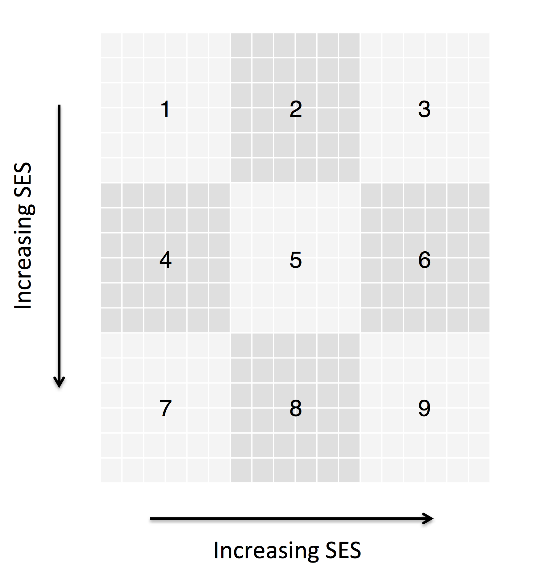
Figure 1. District Geography of Model I Model Analysis: Who Survives?
- 3.5
- One might think that the results of such a simulation are trivial: If everyone chooses based on achievement, there is perfect information and mobility, and if existing schools have no limits on capacity, then the school with the highest mean achievement (School 9) will end up with all the students in a just a few time periods. Figure 2 shows the frequency of survival by school across 100 runs of the model. The runs differ only on account of the stochasticity introduced when initializing student location and achievement. Interestingly, despite having the highest initial mean achievement, School 9 is not the school that survives the largest number of times.
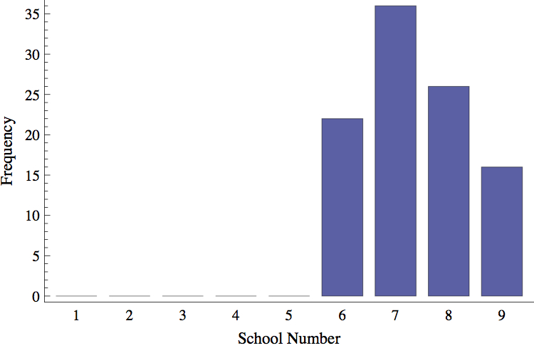
Figure 2. Frequency of Survival By School (Model I, 100 total runs) - 3.6
- The explanation for School 9's failure to win every run becomes apparent after investigating the step-by-step process of how the results emerge. In a world of perfect information and perfect mobility where everyone chooses, all the new incoming students, including low achieving ones, rush to the highest-achieving school. This lowers the mean achievement of School 9, often enough to give one of the other schools a chance to take the lead. In the next time step, all new incoming students rush to the new achievement leader, producing the same dynamic. Consequently, none of the initially highest achieving schools are guaranteed a to be the survivor.
Adding School Effects
- 3.7
- Currently, there are no "school effects" in the model – schools simply report the mean of the achievement of the students. An alternative assumption is that not only do schools help produce achievement gains for the students who attend them, but they also differ in their ability to do so. We incorporate such school effects in Model I by giving a school an additional attribute: value-added.
- 3.8
- The value-added of a school in Model I is defined as the amount (in standard deviation units) that a student's achievement increases each year they attend a particular school. Like achievement, value-added varies across the neighborhoods. School 9 in Neighborhood 9 is given the highest value- added – School 1 in Neighborhood 1, the lowest – with a constant decrease in between. Thus, School 9 is not only the school initialized with the highest achieving students, but has also become the one with the indisputably highest value-added of any school in the district.
- 3.9
- Figure 3 illustrates what happens to school enrollments on a typical run of the simulation with school effects activated but all other rules exactly as before. The lowest achieving schools, Schools 1-6, die out quickly, while School 7 remains for approximately 40 time periods. The two highest achieving and highest value-added schools – Schools 8 and 9 – survive, and their enrollments fluctuate from year to year.[3] School 9 has a higher initial mean achievement, a higher value-added, and can grow instantly to accommodate all the students in the district. Yet another school not only persists but alternates with School 9 for the lead in total enrollment. The same dynamic identified when there were no school effects is largely responsible for this outcome as well – the school with the highest mean achievement draws students that lower its mean achievement, making another school the highest achieving the following year. The addition of school effects simply slows down the decrease in mean achievement enough to enable more than one school to survive.
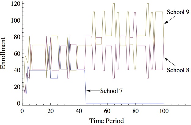
Figure 3. Student Enrollments by School (School Effects "On") - 3.10
- To be clear, we are not using Model I to claim that such an oscillation in enrollments is likely to happen in the transition to a public choice program. At a minimum, one would need much more detailed information about how students make school choices in order to make such a prediction. Instead, Model I suggests that even in this very simple case where individual decision-making is perfectly understood, the district-level aggregation of those decisions is not straightforward. Moreover, the converse is also true. Imagine the inferences one might make about school actions if one witnessed such alternating leads in enrollment amongst real world schools. Likely explanations would include fluctuating school quality or competitive actions by schools to win back students. Our model shows that neither of those factors is necessary to generate the observed data. Indeed, oscillation is the appropriate baseline model for a system where everyone chooses in a similar manner and with very little friction (i.e., no mobility costs, no capacity constraints, etc.). In short, by enabling the exploration of how a wide range of student- and school- level actions aggregate into district-level outcomes, insights from agent-based models help us better interpret real world outcomes that emerge in the transition from catchment area to choice-based systems.
Model II: The transition to public school choice
- 4.1
- Model II builds upon Model I in two broad ways. First, we ensured that the initialization of the model parameters, such as student achievement and school value-added, corresponded with a set of reasonable, real world values – in this case, data on students and schools from Chicago Public Schools (CPS) open enrollment program during the years of 2000 to 2003. During this time period, over 15,000 students per year enrolled in the 9th grade of CPS high school, with approximately 55% of them choosing to attend a school other that the one to which they were assigned. Second, some public choice programs – like the one in Chicago – are accompanied by a parallel effort to open charter schools with more freedom to operate their school in a manner the founders see fit. Consequently, in Model II, we allowed for new schools to enter the district. To ensure that this mechanism could introduce system improvement, we assumed that the new schools would have a high value-added relative to incumbent schools.[4]
Model Description
- 4.2
- As in Model I, there are two types of agents – students and schools – that operate on a landscape that represents the geography of the district. The simulation begins in a state where all students attended their assigned neighborhood school, and the first time period of the simulation represents the first year an incoming cohort of students can choose. An overview of the model is presented first, followed by the precise specification of the agent rules in subsequent sections.[5]
- 4.3
- Each time period of the simulation proceeds as follows:
- The model is populated with incoming students, a fraction of whom are randomly designated as "choosers"; this fraction is determined by the exogenous parameter, pc
- The choosers rank schools in accordance to their preferences and, in random order, attempt to attend their top choice school; the non-choosers attend their assigned neighborhood school.
- If there are no available spaces at the student's top choice, the student attempts to attend the next school on their ranked-list, and continues to try schools until they find one with room. Regardless of availability, a student's assigned neighborhood school must accept them.
- Students update their achievement level; the updated achievement depends both on the student's individual attributes and the value-added of the school they attend.
- Schools update their aggregate enrollment and achievement values; they also estimate the number of spaces available for new students next year.
- Students completing their fourth year in a school graduate from the system; a student stays at the same school until graduation.
- Schools that do not meet a minimum threshold of enrollment are permanently closed.
- New schools open in random geographic locations; the number of new school introduction rate is determined by the exogenous parameter, nsr
Student Attributes and Initialization
- 4.4
- To populate the model with new incoming students in each time period, Model II sampled from a set of 17,131 incoming 9th grade students identified from data made available by Chicago Public Schools.[6] To enter the set of 17,131, a student had to (a) attend 9th grade at a CPS high school between the years of 2000 and 2003, (b) attend a CPS school in the 8th grade, (c) remain in the same home census block between 8th and 9th grade, and (d) have valid and non-missing 8th and 11th grade standardized test scores. The goal was to create initial conditions that resembled a district where students attended assigned, neighborhood schools so students who attended magnet and selective schools where not included.
- 4.5
- A given student i in the simulation has the following attributes, corresponding to the actual CPS student data:
- {xcori , ycor i }: the geographic location based on the student's home census block
- achiev1i : incoming achievement
- achiev2i : current achievement as determined by the simulation
- povertyi : the concentration of poverty in the student's home census block
- assignedi : neighborhood school assigned to the student by the district
- attendedi : actual school attended by the student as determined by the simulation
- whitei : 1 = white, 0 = other race
- malei : 1 = male, 0 = female
School Attributes and Initialization
- 4.6
- The simulated district consists of 43 neighborhood schools, all of who had students that were a part of the 17,131-student sample. A given school j in the simulation has the following attributes, corresponding to the actual CPS data:
- {xcorj , ycorj }: the geographic location of the school
- enrollj : the total number of students enrolled in the school
- maj : the mean achievement of all the students that attend the school
- vaj : the value-added of the school; partially determines the achievement of students attending that school
- dcj : the design capacity of the school's building
- attdassgnj : the number of incoming students assigned to the school that actually attended the school
- expassgnj : the mean of attdassgnj from the last four time periods; represents the number of students assigned to the school expected to attend the school in the following time period
- availspj : the number of available spaces for the incoming cohort of students
- closedj : 1 = permanently closed, not accepting new students; 0 = open and accepting new students
- newj : 1 = school created after time 0, 0 = initial school
- 4.7
- The approximate value-added of each school, vaj, was obtained by estimating a hierarchical linear model that predicts 11th grade Prairie State Achievement Examination scores for all students used in the simulation, using the 8th grade Iowa Test of Basic Skills scores and student- level demographics of those students as the independent variables (Table 1). The school-level residuals of that model were used as estimates of vaj for each school, and the resulting estimates were also used in the student achievement growth rule below (Eq. 1).[7]
Table 1: Hierarchical Linear Model of 11th Grade PSAE Math Scores (17143 students, 43 schools) Estimate Standard Error Fixed Effects Intercept -0.0956 0.0301 8th Grade ITBS 0.6794 0.0053 White 0.1567 0.0183 Male 0.1151 0.0097 Poverty -0.0629 0.0080 Random Effects School-level residual variance 0.0363 Student-level residual variance 0.3921 - 4.8
- Schools were initialized by running the model for five time periods, under the condition that students were forced to attend their assigned school. A representative initialization of the district is presented in Figure 4.
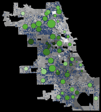
Figure 4. Representative Initialization for Model II. A circle represents a school. The circle's size is proportional to the school's enrollment, and its color indicates the mean achievement of the school (light green, high; dark green, low). Schools are placed at the geographic location of their address. The small blue dots represent students, who are placed within their home census block and attend their assigned school. The color of the census block indicates the poverty of the location (dark gray, high; light gray, low). Student Rules
Achievement growth
- 4.9
- Current achievement is updated only once for each student, at the completion of the first year at the school, and remains constant thereafter. The achievement level of a student is a function of their own characteristics and the value-added of the school they attend. More specifically, the current achievement for student i attending school j is determined using the following equation estimated from CPS data as described in Table 1:

(1) where rij is determined by a random draw from a normal distribution with mean zero and standard deviation of 0.626179 every time the achievement growth equation is calculated. The standard deviation comes from the estimate of the student-level residual variance in the hierarchical linear model.
School choice
- 4.10
- Incoming students select a school to attend and remain at the school for four years. Students who are not choosers attend their assigned neighborhood school. Students who are randomly designated as choosers, rank schools using a utility function that trades off between the mean achievement of the school, and its geographic proximity to the student, given by:
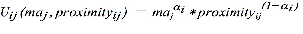
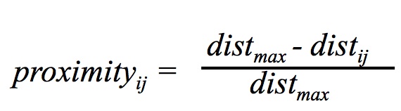
(2) where αi is a student specific value determined by drawing from a normal distribution with mean α and a standard deviation of 0.05. α is an exogenously determined parameter that alters the weight given to the mean achievement of the school relative to the geographic proximity of the school to the student. proximityij is a function of distij, the Euclidian distance between a student and a school[8], and is normalized with respect to distmax, the maximum distance between two points in the district:
(3) After ranking their schools, the choosers "apply" to their top choice school. Students apply to schools in random order at the start of each time period. If the school accepts them, the students reduce the available spaces, availspj, at that school. If the school does not accept them, students apply to the next school on their utility-ranked list. Regardless of availability, a student's assigned neighborhood school must accept them.
School Rules
New School Formation
- 4.11
- Each time period, nsr number of new schools open in randomly chosen locations at the end of each time period. Since these schools have no student achievement history, an assumption must be made about how to initialize their mean achievement. The exogenous parameter opt (optimism) determines the quantile of the existing school mean achievement distribution to use for this assumption. For example, if opt = 0.5, new schools will be initialized with the median value of the mean achievement of all open schools. In subsequent periods, the mean achievement of the new school equals the mean of the students who chose to attend that school. Regardless of the value of opt, the design capacity of a news school, dcj, is always set to the median design capacity of the other open schools in the district.
- 4.12
- In order to introduce a mechanism for improvement, one school is chosen at random from the schools in the top decile of current value-added distribution. The value-added for a newly created school is a random draw from a normal distribution that has a mean equal to the mean achievement of the school chosen from the top decile. The standard deviation of the distribution is equal to the standard deviation of value-added distribution across the set of schools used to initialize the simulation. One way to interpret this is that the new schools attempt to "copy" the best schools. Sometimes, they "innovate" by doing even better than those they copy; other times, they do not perform as well. The assumption to have new schools born into the system with higher value-added reflects our desire to understanding how the dynamics unfold under a "best case" scenario.
School acceptance policy
- 4.13
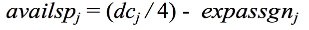
- Schools must accept students that are assigned to them. Students assigned to other neighborhood schools are accepted on a first-come, first-served basis, as long as there is space available in the 9th grade. Space is limited by the design capacity of the school, dcj. Additionally, since there is only one round of application and acceptance within each time period, schools must forecast the number of students assigned to them that will actually attend their school. This forecast is based on the mean of the number of incoming assigned students who attended their school in the previous four years, expassgnj. The available space at the beginning of any given time period is then given by:
(4) No other selection criteria are used.
School closure
- 4.14
- Schools permanently close if their total enrollment in all grades drops below the exogenously determined fraction of their design capacity, ct. The only exception to this is for new schools, that are given a four-year "incubation" period during which they are exempt from the minimum enrollment threshold. Incoming students who are assigned to a closed incoming school, are reassigned randomly to one of the two geographically nearest schools.[9]
Model Analysis
- 4.15
- Since our primary interest is in understanding how district-level mean achievement might vary depending on school choice decision rules used by the choosers, we generated data by running the model for fifty time periods under various combinations of student-level emphasis on achievement (α) and percent choosers (pc). Each unique combination of parameters was repeated one hundred times to create a distribution of outcomes. We began with the assumptions that new schools would be readily available for students (nsr = 4), that it is very difficult to close schools (ct = 0.05), and that households would perceive new schools as having the median value of the mean achievement of current schools (opt = 0.5).
- 4.16
- Figure 5 presents the main result: district-level mean achievement does not necessary increase as the student-level emphasis on school achievement (α) increases. Figures 6 and 7 explain the reason for this unexpected micro-macro relationship: High levels of α lead to new schools that enter the system early in the process. Since new schools improve upon each other's value-added over time, high α therefore often leads to a final population of schools with lower quality than low α. Figures 8– 10 examine the sensitivity of the primary finding to changes in the assumptions about the rate at which new school are introduced into the system (nsr), the ease with which school can close (ct), and the optimism about the performance of new schools with no achievement history (opt). We find that this counterintuitive relationship between student-level emphasis and district-level outcomes is most likely to be observed when the percentage of households is moderate to low, schools do not close very easily, and new schools are introduced a high rate. It is least likely to be observed when the fraction of households choosing is high and households are very optimistic about the unknown quality of new schools.
Table 2: Summary of Experimental Parameters pc Percent choosers: the percentage of incoming students who can actively choose a school α Emphasis on student achievement: the weight placed on the mean achievement relative to geographic proximity by the students. αi for any individual student is determined by drawing a value from a normal distribution with mean α and a standard deviation of 0.05; the higher the α, the more students value achievement ct Closing threshold: the fraction of the building enrollment design capacity at which a school will close; the higher the ct, the easier schools are to close nsr New school introduction rate: the number of new schools that open per year opt Optimism: the quantile of the current mean achievement distribution (across schools) assigned by students to a new school in its first year District Outcomes versus Student-level Emphasis on School Achievement
- 4.17
- Figure 5 plots the mean achievement of all students in the district at the end of fifty time periods, against the student-level emphasis on mean achievement when choosing a school (α). Each point represents the average of the 100 runs for a given value of α and percent choosers (pc). As might be expected, as the percentage of students choosing increases so does the mean achievement of the district. Part of this increase comes from students moving into higher value-added existing schools, and part comes from the fact this student movement also enables the survival of new, higher-value added schools. As the student-level emphasis on achievement increases within a particular level of percent choosers, however, the results are more mixed. For all but the highest level of pc, the mean achievement reaches a peak in low to mid-values of α. After a certain point, the more the population of students emphasizes achievement in their decision-making process, the lower each becomes. Understanding the reason for this unexpected micro-macro relationship requires on delving into the impact of α on the timing and volume of new school entry. Lower levels of α lead to fewer new schools surviving that were created later in the process. Since the value-added of the new school depends on the existing value-added distribution of the school population, schools formed later will more likely be of higher value-added than ones formed earlier. Consequently, the value-added of the new schools created will decrease as α increases, unless other factors enable the creation of new schools later in the process.
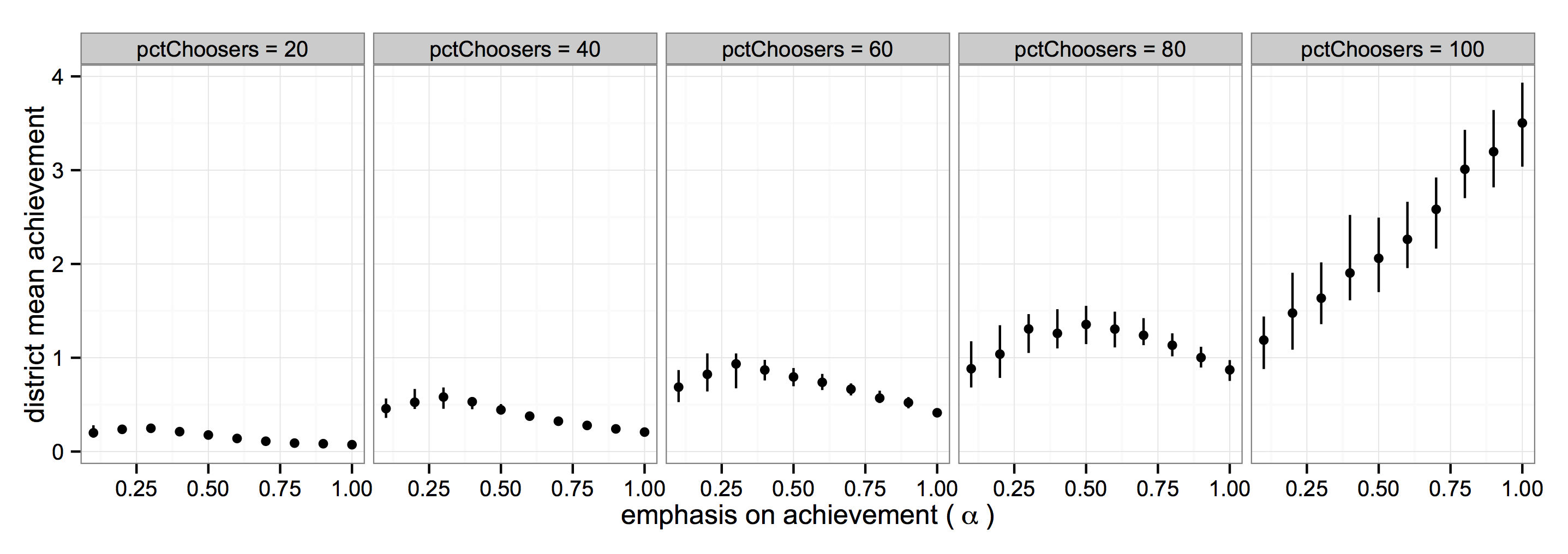
Figure 5. District Mean Achievement vs. Emphasis on Achievement, by Percent Choosers (nsr = 4, ct=0.05, opt = 0.5, 100 runs) - 4.18
- Figures 6 and 7 further illustrate this point. Figure 6 focuses on the timing of new school entry. Each column represents each of the pc conditions in Figure 5. The plots in the first row of Figure 6 show the mean of the value-added distribution of the surviving new schools after fifty time periods. Each plot in the second row of Figure 6 shows the mean age of the surviving new schools for each condition of α. The data points on all the plots are the average values across the 100 runs. The graph suggests that, generally speaking, lower α leads to younger distributions of surviving new schools. Moreover, the changes in mean school age almost perfectly mirror the changes in mean value-added: the younger the mean age, the higher the final median value-added. The exceptions to this pattern are the dips observed for certain ranges of α in the second row of Figure 6. The dips are caused by closures of initial schools that occur later in the process, closures that enable the survival of new schools created with higher value-addeds. For low α and low pc, very few closures occur, and those that do occur happen early in the process. As the percentage of choosers increases, more delayed closures occur, creating a deeper and deeper dips. When the pc gets high enough, closures continue well into the process – that is, even the new, high-value-added schools close and are replaced by newer schools. This leads to the continuous growth in value-added observed in the pc equals 100 condition in Figure 6.[10]
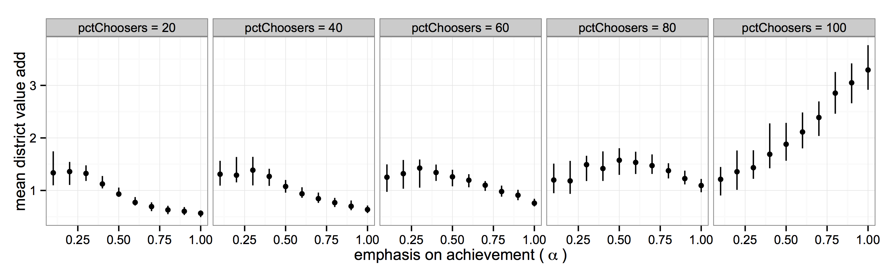
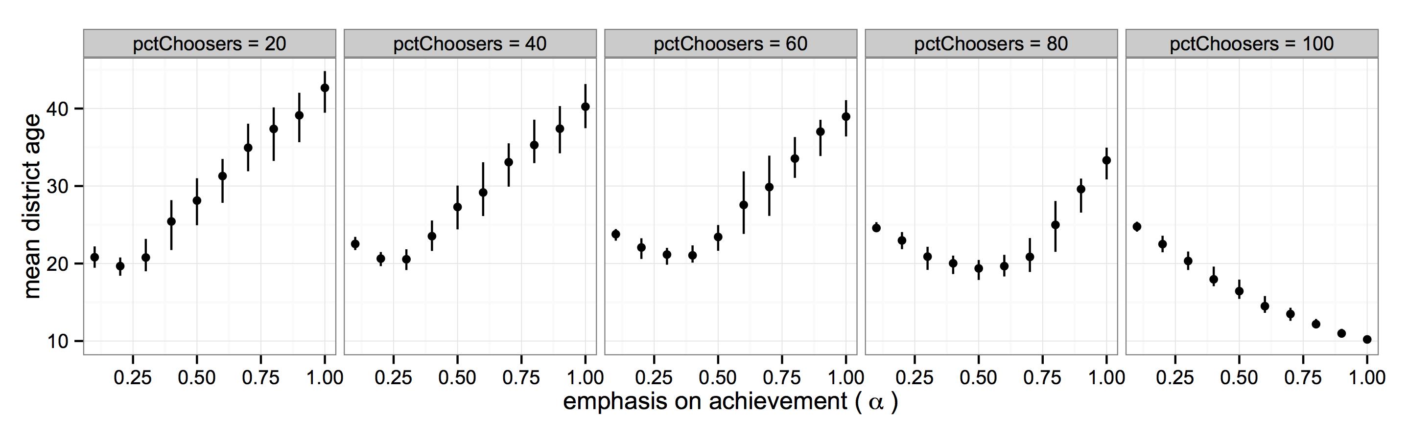
Figure 6. Mean Value-Added and New School Age vs. Emphasis on Achievement, by Percent Choosers (nsr = 4, ct=0.05, opt = 0.5, 100 runs) - 4.19
- Figure 7 focuses on the total number of new schools. It shows the growth of new schools over time from a representative run from a low α, medium α, and high α condition. For the low α condition, the number of new schools keeps climbing over time. For the higher α conditions (α = 0.5 and α = 1), the number of new schools grows in the initial time periods but then levels off. Why does a lower α lead to more new schools? Consider the decision of an individual student when a new school, N, is introduced. Suppose that the student's top available choice, School A, is currently a school with an above-median mean achievement. Furthermore, School N is both geographically closer than School A and has a much higher value-added (given that, since the school has no achievement history, in the first time period of its life, School N's mean achievement is perceived as equal to the median achievement of all schools). In the extreme case where α = 1, there is virtually no chance that the student attends School N over School A even though it is closer and has a higher value-added – i.e., if all that matters in the utility function is the mean achievement of the target schools, the student will only attend School N if her next best choice is below the median mean-achievement. In subsequent periods, however, School N's mean achievement may rise (especially given the school's higher value- added) and students left with a similar decision may instead choose it over School A. But initially, this situation creates a handicap for School N when compared to incumbent, high mean achievement schools. Moreover, that handicap may very well lead to its extinction at the end of its initial incubation period. As α decreases, however, School N's attractiveness to the student (and others like her) increases, along with the chances for School N's survival.
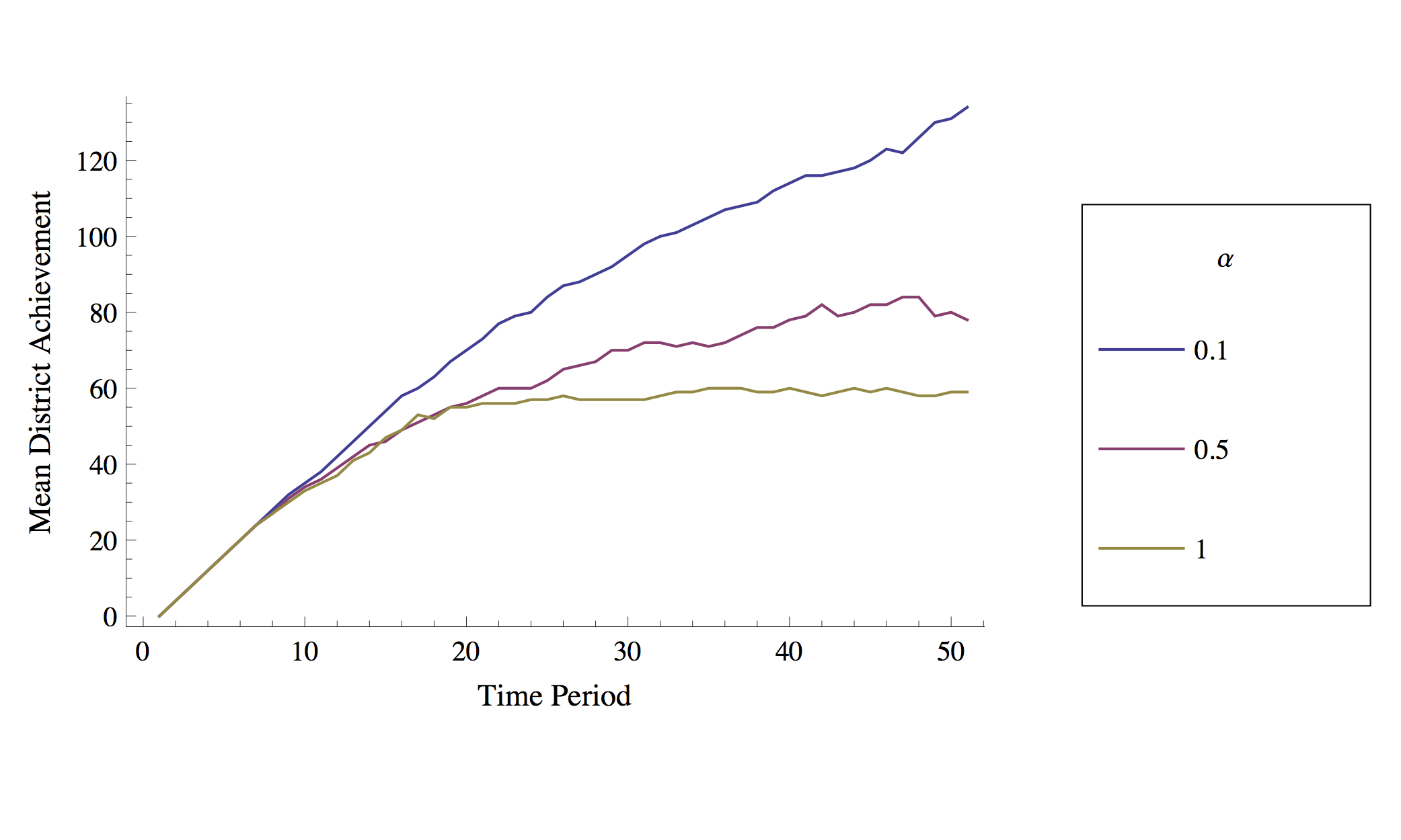
Figure 7. Number of New Schools vs. Time
Representative dynamics for 3 levels of α; nsr = 4, ct=0.05, opt = 0.5, pc = 80. - 4.20
- As Figures 6 and 7 show, the percentage of students participating in the choice program and the emphasis those students place on school achievement play an important role in determining the size and age of the surviving new-school population. In the next three sections, we more closely examine the impact of varying three additional factors in the model that can influence the quantity and timing of the new schools, and hence the final mean value-added and mean achievement of the district: the rate at which new schools attempt to enter the system, nsr; the assumption households make about the quality of new schools, opt; and the ease with which low enrollment schools close, ct. Our primary interest in the sensitivity analyses that follow is to examine the robustness of the counterintuitive finding that a higher student-level emphasis on school achievement does not always result in a higher district-level achievement even when new schools that enter the district are higher quality than incumbent schools.
Sensitivity to New School Introduction Rate
- 4.21
- The rate at which new schools enter the system has the potential to impact the results of the simulation in at least two ways. First, every new school represents an additional opportunity for improvement. More new schools could lead to higher district-level mean achievement in time period fifty. Second, every new school also adds capacity to the system which could impact the number of existing school closures.
- 4.22
- Figure 8 shows the impact of varying the number of new school introduction rate (nsr) under five different levels of percent choosers. The lines on the plots depict the relationship between α and district-level mean achievement, with each line corresponding to a different value of nsr. The darker the line, the faster new schools are introduced into the system. Note that finding about the relationship between student-level emphasis on achievement (α) is not very sensitive to the level of nsr – the shape of the lines in Figure 8 essentially mirror the ones in Figure 5. To the extent that nsr does alter the results, its impact is contingent the level of α. For low levels of α, introducing schools faster leads to higher district mean achievement. The differences in district mean achievement across levels of nsr narrow and essentially become indistinguishable, however, as α increases. The underlying reason is exactly as before. When α is high, new schools created early in the process are more likely to survive, as more students leave their assigned schools. The higher the nsr, the greater the number of early entrant survivors, and the fewer the number late entrants (with higher value-added) that survives. The exception to this pattern is also as before: if enough students choose (e.g., the case of 100 pc), α and district achievement increase together on account of the continuous turnover in schools.
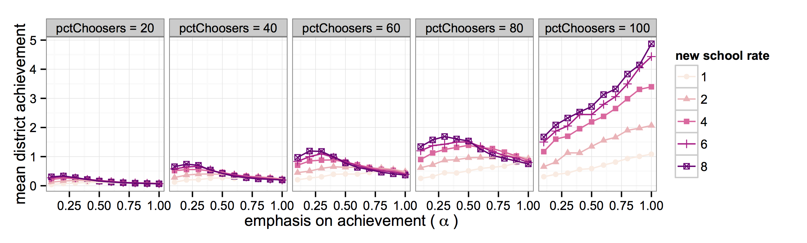
Figure 8. Mean District Achievement vs. Emphasis on Achievement, by New School Rate and Percent Choosers (ct = 0.05, opt = 0.5, 100 runs) Sensitivity to Ease with which Schools Close
- 4.23
- The decision to close a school is complex one that involves balancing the needs and desires of a number of competing interests in a community. We have abstracted away that complexity in our model buy assuming a school closes if its enrollment drops below a certain fraction of the building design capacity (the closing threshold, ct). Moreover, in the results presented so far we have set the closing threshold to 0.05 to understand the emergent district-level outcomes when school closure is extremely difficult. While not capturing the full complexity of the (often political) forces that determine the closure of public schools in the United States, increasing ct can give us some sense of how outcomes vary in cases when schools are easier to close.
- 4.24
- The lines on the plots in Figure 9 depict the relationship between the student-level emphasis on school achievement (α) and district-level mean achievement under five different levels of percent choosers. The darker the line, the easier it is for schools to close. Figure 9 shows that the relationship between student emphasis on achievement and district-level mean achievement is much more sensitive to changes in ct, than with changes in the rate at which new schools are introduced (Figure 8). However, the finding that a higher emphasis on achievement does not always translate into better district-level performance continues to hold true for a significant number of cases. Closing thresholds of 0.4 and below in the 20 and 40 percent chooser cases and closing thresholds of 0.2 and below in the 60 percent choosers case, show either a decreasing, flat, or slightly curvilinear relationship between α and district-level achievement. Moreover, these conditions represents a range of plausible real world situations: in the data used to initialize the simulation, 36% of the Chicago students attended schools other than their assigned school, and 7 of the 43 schools had enrollments less than 40% of their capacity.
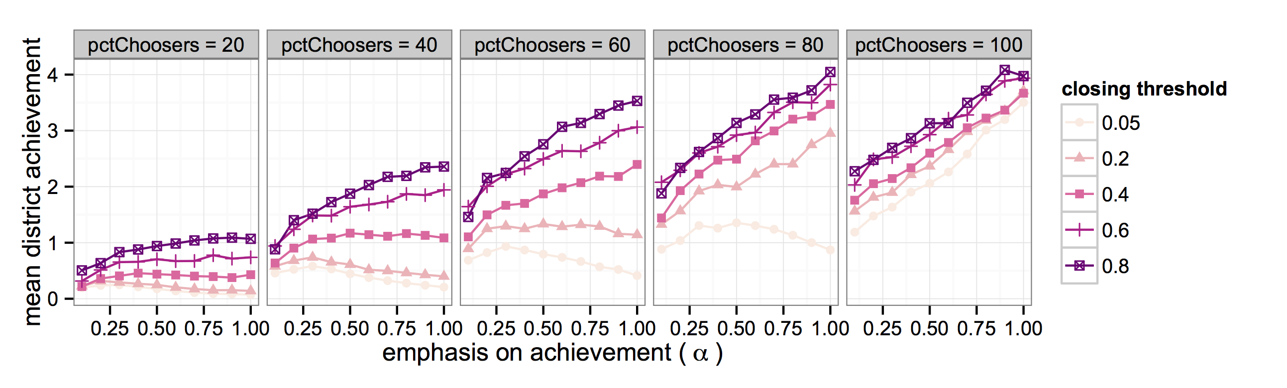
Figure 9. Mean District Achievement vs. Emphasis on School Achievement, by Closing Threshold and Percent Choosers (nsr = 4, opt = 0.5, 100 runs) Sensitivity to Optimism about New Schools
- 4.25
- Because of the lack of performance history for new schools, their quality is initially unknown. Up to this point, students treat a new school as if it has a mean achievement equal to the median mean achievement across all open schools (opt = 0.5). We can vary the optimism of this assumption by changing the quantile of the current school mean achievement distribution. Quantiles above the median will make it more optimistic than our initial assumption; quantiles below, more pessimistic.
- 4.26
- Figure 10 shows the impact of varying optimism (opt) under five different levels of percent choosers. The lines on the plots depict the relationship between student-level emphasis on achievement (α) and district-level mean achievement, with each line corresponding to a different level of optimism. The darker the line, the more optimistic students are about the performance of a new school. As was the case with increasing the closing threshold, the relationship between α and district-level mean achievement changes as the level of optimism changes. More specifically, as optimism increases the peak of the curve moves to the right until reaching the point where mean achievement continues growing as α increases. However, once again we see that a substantial number of conditions result in a curvilinear or negative relationship between student emphasis on achievement and district mean achievement. Even in the 100 percent choosers case, enough pessimism by the students can lead to a downward sloping line.
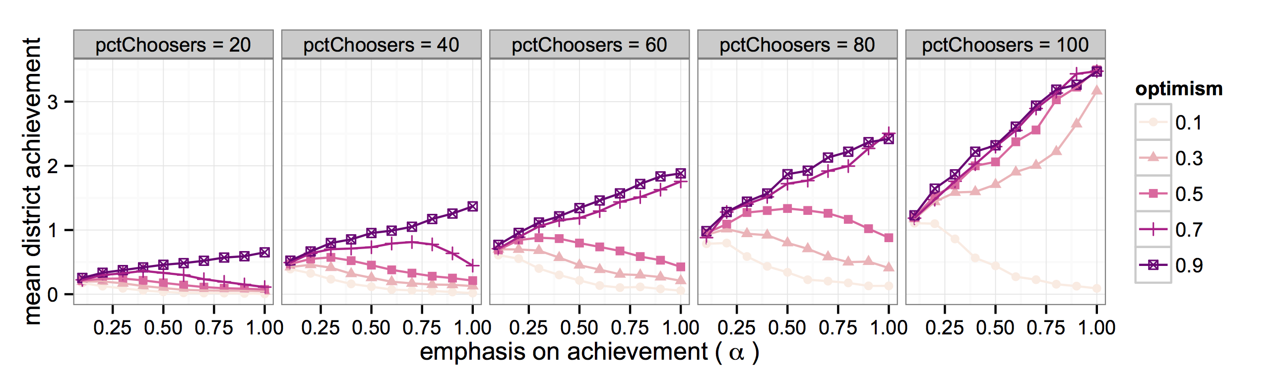
Figure 10. Mean District Achievement vs. Emphasis on Achievement, by Optimism and Percent Choosers (nsr=4, ct = 0.05, 100 runs)
Discussion and conclusion
- 5.1
- By developing an agent-based model of the transition from catchment-area to public school choice systems, this paper contributes to our understanding of the dynamic processes that lead to district-level outcomes. Analysis of our model reveals the importance of considering the timing of new schools' entrance into the system, in addition to their quantity and quality. Timing matters because, assuming that system improvement comes from imitating and improving the top performers, late entrants have an opportunity to imitate a population of higher quality schools.
- 5.2
- Our model further demonstrates how the existence of late entrants in the final school population depends on a combination of the fraction of students participating in the choice program (pc), the emphasis those households place on school achievement (α), the assumptions those households make about the quality of new schools (opt), how easily schools close (ct), and the rate at which new schools attempt to enter the system (nsr). Given the assumption that the new schools are higher quality than incumbents, computational experiments sweeping across values of these factors reveal some expected results. District mean achievement increases as more students take advantage of the opportunity to choose, as students become more optimistic about the performance of new schools, and as incumbent schools become easier to close. However, analysis of the model also reveals a paradoxical mismatch between student-level and district-level behavior. For a range of plausible real-world conditions, the more students emphasize school achievement relative to geographic proximity in their school-choice decisions, the lower the mean achievement of the district. This result is most likely to be observed when the fraction of households is moderate to low, schools do not close very easily, and new schools are introduced a high rate. It is least likely to be observed when the fraction of students choosing is high and students are very optimistic about the unknown quality of new schools.
- 5.3
- While our results are generally suggestive of a district strategy that attempts to spread out initial school closures and new school openings over time, several limitations of our work should be addressed before attempting to use agent-based models such as this one to make more precise statements about school district planning. First, we reiterate that we all our results are contingent on the assumption that new schools have a higher value-added on average than incumbent schools. This assumption reflects our desire to better understand how the dynamics of school choice unfold under a scenario where one would expect choice to lead to district improvement. It should not be misinterpreted as implying that in Chicago or other school districts new schools are necessarily better schools. Moreover, the model assumes new schools attempt to improve upon the practices of the existing top performers in the district. Even if one assumes that new schools have a higher value-added, our results could be different if the new schools were allowed to continuously introduce unfamiliar innovations imported from outside the district. However, this limitation is more likely to matter when modeling small and homogeneous school districts, than it is when modeling large urban districts whose schools already engage in a very wide and rather representative variety of available reforms.
- 5.4
- Second, the model does not yet address the possibility of internal school improvement in response to competitive pressures. A mechanism for internal improvement could be incorporated into the current model by introducing a rule – potentially calibrated to be consistent with work attempting to estimate the magnitude of the competitive response (e.g., Figlio & Rouse 2006) – that enabled schools losing students to respond by increasing their value-added. However, to the extent one were willing to believe that improvement comes largely from new entrants as opposed to incumbents, this concern is mitigated.
- 5.5
- Third, a much more refined understanding of student preferences is required. Our current model only partially addresses heterogeneity in the decision-making rules of households. Additional heterogeneity could come in the form of criteria by which to judge schools that go beyond mean achievement and geographic proximity, such as similarity in socioeconomic status. Additionally, student decision-making in the current model is not correlated to household characteristics, such as socioeconomic status or existing student achievement. While such a correlation is not likely to impact the overall level of district achievement, connecting socioeconomic status to the preferences or ability of a household to select a non-neighborhood school is necessary if one were to use this model in to examine distributional impacts of school choice.
- 5.6
- Finally, the composition of student's peer group, classroom, or school does not directly impact student achievement growth in the model, as the data used in our model did not enable us to parse out such "peer effects" from from the value-added of the school (Zimmer & Toma 2000; Lefgren 2004; Maroulis & Gomez 2008; Wilkinson et al. 2000, for review). Using this model to examining the distributional consequences of school choice would therefore also require the inclusion of peer quality (and/or variance in peer quality) in the achievement growth rule. The model in this study provides a starting point for future work to address such limitations in addition to highlighting the importance of considering the timing of new entrants in a school choice system.
Notes
-
1 We do not make the distinction between a "household" and a "student" in our model, so note that we will use the terms interchangeably.
2 The models in this paper were implemented using the NetLogo multi-agent programmable modeling environment (Wilensky 1999), a widely used and powerful environment used to model a large range of natural and social systems. For a comprehensive introduction, see Wilensky & Rand (in press).
3 Occasionally, School 7 survives and School 8 does not.
4 An alternative improvement mechanism, left for future work, is to have existing schools implement new and improved ways of educating their students in response to competitive pressures.
5 The NetLogo code for Model II can be accessed via the CoMSES Computational Model Library: http://www.openabm.org/model/3695
6 As it will be made clear below, the fact that students get re-used in this process is not a problem since the key attributes – current achievement and attended school – are determined by the simulation.
7 For an overview of the value-added approach in education, see Meyer (1996).
8 Note that Euclidean distance may not correlate perfectly with the time and cost of traveling to a school in an urban area such as Chicago. One alternative for future work would be to use public transportation travel times between origin and destination.
9 School closure also creates a situation where a number of existing, upper-class students are left without a school to attend. One could create a rule for reassignment of those students, but since the numbers are so small relative to the total number of students, we assume that those students instead leave the system. The only consequence of this is that a small number of students is no longer included in the district mean achievement. Since each school determines available space only with respect to the 9th grade (i.e., only incoming, and not existing, students are used in the available space calculation), losing the students does not impact the capacity of the system.
10 This point occurs between 80–100 percent choosers in Figure 6, but that is not always the case. As the sensitivity analysis in Figure 9 illustrates, the exact point where this continuous growth of value-added occurs depends strongly on the closing threshold as well.
References
-
ALEXANDER, K. L., & Pallas, A. M. (1983). School sector and cognitive performance: When is a little a little? Sociology of Education, 58 (2), 115–128. [doi:10.2307/2112251]
ALTONJI, J., Elder, T., & Taber, C. (2002). An evaluation of instrumental variable strategies for estimating the effect of catholic schools (No. 9358). National Bureau of Economic Research. [doi:10.3386/w9358]
BELFIELD, C. R., & Levin, H. M. (2002). The effects of competition between schools on educational outcomes: A review for the United States. Review of Educational Research, 72 (2), 279–341. [doi:10.3102/00346543072002279]
BLIKSTEIN, P., & Wilensky, U. (2010). Materialsim: A constructionist agent-based modeling approach to engineering education. In M. Jacobson & P. Reimann (Eds.), Materialism: A constructionist agent-based modeling approach to engineering education. New York: Springer. [doi:10.1007/978-0-387-88279-6_2]
BRYK, A. S., Lee, V. E., & Holland, P. B. (1993). Catholic schools and the common good. Cambridge: Harvard University Press.
CHUBB, J., & Moe, T. (1990). Politics, markets, and America's schools. The Brookings Institution.
COLEMAN, J. S., Hoffer, T., & Kilgore, S. (1982). High school achievement: Public, catholic, and private schools compared. New York: Basic Books.
COLELLA, V., Klopfer, E., & Resnick, M. (2001). Adventures in modeling. Teachers College Press.
CULLEN, J. B., Jacob, B. A., & Levitt, S. (2006). The effect of school choice on participants: Evidence from randomized lotteries. Econometrica, 74 (5), 1191–1230. [doi:10.1111/j.1468-0262.2006.00702.x]
EPPLE, D., & Romano, R. (1998). Competition between private and public schools, vouchers, and peer-group effects. American Economic Review, 88 (1), 33–62.
EPSTEIN, J. (2006). Generative social science: Studies in agent-based computational modeling. Princeton: Princeton University Press.
EVANS, W. N., & Schwab, R. M. (1995). Finishing high school and starting college: Do catholic schools make a difference? The Quarterly Journal of Economics , 110 , 941–974. [doi:10.2307/2946645]
FERNANDEZ, R., & Rogerson, R. (2003). Equity and resources: An analysis of education finance systems. Journal of Political Economy, 111 (4), 858–897. [doi:10.1086/375381]
FERREYRA, M. (2007). Estimating the effects of private school vouchers in multidistrict economies. American Economic Review, 93 (3), 789–817. [doi:10.1257/aer.97.3.789]
FIGLIO, D., & Rouse, C. E. (2006). Do accountability and voucher threats improve low-performing schools? Journal of Public Economics , 90 (1–2), 239–255. [doi:10.1016/j.jpubeco.2005.08.005]
FISKE, E. B., & Ladd, H. F. (2000). When schools compete: A cautionary tale. Washington, DC: Brookings Institution.
GAMORAN, A. (1996). Student achievement in public magnet, public comprehensive, and private city high schools. Educational Evaluation and Policy Analysis , 14 (3), 185–204. [doi:10.3102/01623737014003185]
GILBERT, N. (2008). Agent-based models. London: SAGE Publications.
GOLDHABER, D. D. (1996). Public and private high schools: Is school choice an answer to the productivity problem? Economics of Education Review, 15 (2), 93–109. [doi:10.1016/0272-7757(95)00042-9]
GREENE, J. P., Peterson, P. E., & Du, J. (1999). Effectiveness of School Choice The Milwaukee Experiment. Education and Urban Society, 31(2), 190–213. [doi:10.1177/0013124599031002005]
HARLAND, K., & Heppenstall, A. J. (2012). Using Agent-Based Models for Education Planning: Is the UK Education System Agent Based? In Agent-based models of geographical systems (pp. 481–497). Springer Netherlands.
HENRICKSON, L. (2002). Old wine in a new wineskin: College choice, college access using agent-based modeling. Social Science Computer Review, 4 (400–419). [doi:10.1177/089443902237319]
HOWELL, W., Wolfe, P., Campbell, D., & Peterson, P. (2002). School vouchers and academic perfor-mance: Results from three randomized field trials. Journal of Policy Analysis and Management, 21 (2), 191–217. [doi:10.1002/pam.10023]
HOXBY, C. M. (2003). School choice and school productivity: Could school choice be a tide that lifts all boats? In C. M. Hoxby (Ed.), The economics of school choice. Chicago: The University of Chicago Press. [doi:10.7208/chicago/9780226355344.003.0009]
HOXBY, C. M. (2005). Competition Among Public Schools: A Reply to Rothstein (2004) (Working Paper No. 11216). National Bureau of Economic Research. Retrieved from <http://www.nber.org/papers/w11216>
JONES, T., & Laughlin, T. (2009). Learning to measure biodiversity: Two agent-based models that simulate sampling methods and provide data for calculating diversity indices. The American Biology Teacher, 71 (7), 406–410. [doi:10.2307/20565343]
KRUEGER, A., & Zhu, P. (2004). Another look at the New York City school voucher experiment. American Behavioral Scientist, 47 (5), 658–698. [doi:10.1177/0002764203260152]
LEFGREN, L. (2004). Educational peer effects and the Chicago public schools. Journal of Urban Economics, vol. 56(2), 169-191. [doi:10.1016/j.jue.2004.03.010]
LEMKE, J. L., & Sabelli, N. (2008). Complex systems and educational change: Towards a new research agenda. Educational Philosophy and Theory, 40 (1), 118–129. [doi:10.1111/j.1469-5812.2007.00401.x]
MAROULIS, S., Guimera, R., Petry, H., Stringer, M., Amaral, L., Gomez, L., Wilensky, U. (2010). A Complex systems view of educational policy research. Science, 330 (6000), 38–39. [doi:10.1126/science.1195153]
MAROULIS, S., & Gomez, L. M. (2008). Does "Connectedness" Matter? Evidence from a Social Network Analysis within a Small-School Reform. Teachers College Record, 110(9), 1901–1929.
MEYER, R. H. (1996). Value Added Indicators of School Performance. Board on Science, Technology, and Economic Policy & National Research Council (Eds.), In Improving America's Schools: The Role of Incentives. National Academies Press.
MONTES, G. (2012). Using Artificial Societies to Understand the Impact of Teacher Student Match on Academic Performance: The Case of Same Race Effects. Journal of Artificial Societies and Social Simulation, 15(4) 8. https://www.jasss.org/15/4/8.html
MORGAN, S. L. (2001). Counterfactuals, causal effect heterogeneity, and the catholic school effect on learning. Sociology of Education , 74 , 341–374. [doi:10.2307/2673139]
NEAL, D. (1997). The effects of catholic secondary schooling on educational achievement. Journal of Labor Economics, 15 (1), 98–123. [doi:10.1086/209848]
NECHYBA, T. (2000). Mobility, targeting, and private-school vouchers. The American Economic Review, 90 (1), 130–146. [doi:10.1257/aer.90.1.130]
NECHYBA, T. J. (2003). What Can Be (and What Has Been) Learned from General Equilibrium Simulation Models of School Finance? National Tax Journal, 56(2), 387–414. [doi:10.17310/ntj.2003.2.06]
ROTHSTEIN, J. (2005). Does competition among public schools benefit students and taxpayers? A comment on Hoxby (2000) (Working Paper No. 11215). National Bureau of Economic Research.
ROUSE, C. E. (1998). Private school vouchers and student achievement: An evaluation of the Milwaukee parental choice program. Quarterly Journal of Economics, 113, 553–602. [doi:10.1162/003355398555685]
SENGUPTA, P., & Wilensky, U. (2009). Learning electricity with NIELS: Thinking with electrons and thinking in levels. International Journal of Computers for Mathematical Learning, 14 (1), 21–50. [doi:10.1007/s10758-009-9144-z]
STONEDAHL, F., Wilkerson-Jerde, M., & Wilensky, U. (2009, May). Re-conceiving introductory computer science curricula through agent-based modeling. In Proceedings of the Eighth International Conference on Autonomous Agents and Multi-agent Systems (AAMAS) - EduMAS Workshop, Budapest, Hungary.
WILENSKY, U. (1999). NetLogo. [computer software]. http://ccl.northwestern.edu/netlogo. Center for Connected Learning and Computer-Based Modeling, Northwestern University, Evanston, IL.
WILENSKY, U., & Papert, S. (2010). Restructurations: Reformulations of knowledge disciplines through new representational forms. In J. Clayson & I. Kalas (Eds.), Proceedings of the con- structionism 2010 conference (p. 97).
WILENSKY, U., & Rand, W. (in press). Introduction to agent-based modeling: Modeling natural, social, and engineered systems with NetLogo. MIT Press.
WILENSKY, U., & Reisman, K. (2006). Thinking like a wolf, a sheep or a firefly: Learning biology through constructing and testing computational theories – an embodied modeling approach. Cognition and Instruction, 24 (2), 171–209. [doi:10.1207/s1532690xci2402_1]
WILENSKY, U., and Resnick, M. (1999). Thinking in Levels: A Dynamic Systems Approach to Making Sense of the World. Journal of Science Education and Technology, vol. 8, no. 1, pp. 3–19. [doi:10.1023/A:1009421303064]
WILKERSON, M. (2009). Agents with attitude: Exploring Coombs unfolding technique with agent- based models. International Journal of Computers for Mathematical Learning, 14 (1), 51–60. [doi:10.1007/s10758-008-9142-6]
WILKINSON, I. A. G., Hattie, J. A., Parr, J. M., Townsend, M. A. R., Fung, I., Ussher, C., et al. (2000, 06-00). Influence of peer effects on learning outcomes: A review of the literature (Tech. Rep. No. ED478708)
WITTE, J. F. (1997). Achievement effects of the Milwaukee voucher program. In American economics association annual meeting. New Orleans.
WITTE, J. F., Sterr, T. D., & Thorn, C. A. (1995). Fifth-year Report, Milwaukee Parental Choice Program. Department of Political Science and the Robert La Follette Institute of Public Affairs, University of Wisconsin-Madison.
ZIMMER, R. W., & Toma, E. F. (2000). Peer effects in private and public schools across countries. Journal of Policy Analysis and Management, 19(1), 75–92. [doi:10.1002/(SICI)1520-6688(200024)19:1<75::AID-PAM5>3.0.CO;2-W]