
 Abstract
- Alignment is a widely adopted technique in the field of microsimulation for social and economic policy research. However, limited research has been devoted to understanding the statistical properties of the various alignment algorithms currently in use. This paper discusses and evaluates six common alignment algorithms used in the dynamic microsimulation through a set of theoretical and statistical criteria proposed in the earlier literature (e.g. Morrison 2006; O'Donoghue 2010). This paper presents and compares the alignment processes, probability transformations, and the statistical properties of alignment outputs in transparent and controlled setups. The results suggest that there is no single best method for all simulation scenarios. Instead, the choice of alignment method might need to be adapted to the assumptions and requirements in a specific project.
- Keywords:
- Alignment, Microsimulation, Dynamic Microsimulation, Algorithm Evaluation
Introduction
- 1.1
- Microsimulation models typically simulate behavioural processes such as demographic (e.g. marriage), labour market (e.g. unemployment) and income characteristics (e.g. wage). The method uses statistical estimates of a system of equations and applies Monte Carlo simulation techniques to generate the new populations, typically over time, both into the future and when creating histories with partial data, into the past. These simulation models often include the transition of individuals from one state to another (e.g. unemployed to employed) where each individual is assigned a probability of making such a transition given their underlying characteristics. The simulation of transitions is often modelled through random draw, where higher probabilities will lead to more likely transitions.
- 1.2
- As statistical models are typically estimated on historical datasets with specific characteristics and period effects, projections of the future may therefore contain error or may not correspond to exogenous expectations of future events. In addition, the complexity of micro behaviour may mean that simulation models may over or under predict the occurrence of a certain event, even in a well-specified model (Duncan and Weeks 1998). Because of these issues, methods of calibration known as alignment have been developed within the microsimulation literature to correct for issues related to the adequacy of micro projections.
- 1.3
- Scott (2001) defines alignment as "a process of constraining model output to conform more closely to externally derived macro-data ('targets')." There are both arguments for and against alignment procedures (Baekgaard 2002). Concerns directed towards alignment mainly focus on the consistency issue within the estimates and the level of disaggregation at which this should occur. It is suggested that equations should be reformulated rather than constrained ex post. Clearly, in an ideal world, one would try to estimate a system of equations that could replicate reality[1] and have effective future projections without the need for alignment. However, as Winder (2000) stated, "microsimulation models usually fail to simulate known time-series data. By aligning the model, goodness of fit to an observed time series can be guaranteed." Some modellers suggest that alignment is an effective pragmatic solution for highly complex models (O'Donoghue 2010).
- 1.4
- Over the past decade, aligning the output of a microsimulation model to exogenous assumptions has become standard despite this controversy. In order to meet the need of alignment, various methods, e.g. multiplicative scaling, sidewalk, sorting based algorithm etc., have been experimented along with the development of microsimulation (see Morrison 2006). Microsimulation models using historical datasets, such as the back simulation models in Li and O'Donoghue (2012) and CORSIM (SOA 1997), align the output to historical data to create a more credible profile. Models that work prospectively, e.g. APPSIM, utilises the technique to align their simulation with external projections (Kelly and Percival 2009). Additionally, a microsimulation model that interacts with macro models, e.g. CGE model, may also use alignment to bridge the projections between micro and macro models (Davies 2004; Peichl 2009).
- 1.5
- Nonetheless, the understanding of the simulation properties of alignment in microsimulation models is very limited. Literature on this topic are scarce, with a few exceptions such as Anderson (1990), Caldwell et al. (1999), Neufeld (2000), Chénard (2000a; 2000b), Johnson (2001), Baekgaard (2002), Morrison (2006), Kelly and Percival (2009) and O'Donoghue (2010). Although some new alignment methods were developed in an attempt to address some theoretical and empirical deficiencies of earlier methods, discussions on empirical simulation properties of different alignment algorithms are almost non-existent.
- 1.6
- This paper aims to fill this gap and better understand the simulation properties of alignment algorithms in microsimulation. It evaluates all major binary alignment methods under various scenarios. The comparison includes the alignment processes, probability transformations, and the statistical properties of alignment outputs. Alignment performances are tested using various evaluation criteria, including the ones suggested by Morrison (2006).
- 1.7
- The paper is divided into 6 sections. In the next section, we will review the background to the alignment methodology used in microsimulation and summarize the existing algorithms used in various models. Section 3 discusses the objectives of alignment and the method of algorithm evaluation. Section 4 describes the detail of the datasets used in the evaluation process and some key statistics. We will present the results of the evaluation in section 5, and conclude in the last section.
Alignment in Microsimulation
- 2.1
- This section discusses the purpose of alignment in a microsimulation model and the common practice of their statistical implementation. Alignment is essentially a calibration technique used when the micro model outputs do not conform to expectations. Baekgaard (2002) suggests two broad categories for alignment:
- parameter alignment, whereby the distribution function is changed by adjustment of its parameters; and
- ex post alignment, whereby alignment is performed on the basis of unadjusted predictions or interim output from a simulation.
- 2.2
- This paper focuses on the ex post alignment methods, as they are the most common form of alignments in microsimulation. In most cases, a microsimulation model applies this prediction process to all observations individually without constraint at aggregate level. However, this may lead to a potential side effect: The output of the prediction, although it may look reasonable at each individual level, may not meet the modeller's expectation at the aggregate level. For instance, the simulated average earning might be higher or lower than the assumption. Therefore, alignment is introduced as the step after the initial prediction in order to impose an ex post constraint.
- 2.3
- There might be several reasons why the initial model outputs do not meet the expectations. It could be due to the data on which the equations of the model have been estimated is not representative, or there is a structural change in the behaviour which means the original estimation is now biased. Alignment imposes extra assumptions on the potential source of error and attempts to change the distribution in a consistent way. It is also possible that the initial model has a poor predictive performance due to limited data or even mis-specification. In these cases, alignment is not supposed to be used to fix the problem as the solution lies deep in the modelling procedure. However, given the limits to data availability and complexity of human behaviours, alignment is sometimes used as a last resort to reproduce a reasonable distribution when all other options have been exhausted. Although there are some theoretical debate of ex post alignment usage, alignment is de facto widely adopted in the models built or updated within last decade, e.g. DYANACAN (Neufeld 2000), CORSIM (SOA 1997), APPSIM (Bacon and Pennec 2009). A few papers, e.g. Baekgaard (2002), Bacon and Pennec (2009) and O'Donoghue (2010), have discussed the main reasons for alignment, and summarise them as follows.
- Alignment provides an opportunity for producing scenarios based on different assumptions. Examples include the simulation of alternative recession scenarios on employment with different impacts on different social groups (e.g. sex, education or occupation).
- Alignment can be used as an instrument in establishing links between microsimulation models of the household sector and the macro models. It is a crucial step to reach a consistent Micro-Macro simulation model (see Davies 2004).
- Alignment may be used to address the unfortunate consequences of insufficient estimation data by incorporating additional information in the simulations. Since no country has an ideal dataset for estimating all the parameters needed for microsimulation, modellers often make compromises, which adversely affects the output quality. Alignment, although does not solve the problem, is sometimes used to mitigate the impact of these errors.
- Certain alignment algorithms can also be used to reduce Monte Carlo variability though its deterministic calculation (Neufeld 2000). This is useful for small samples to confine the variability of aggregate statistics.
- 2.4
- The implementations of alignment may vary depending on the variable type and the assumptions imposed in the statistical estimations. Models of continuous events such as the level of earnings or investment income, utilise statistical regressions with continuous dependent variables and produce a distribution of continuous values. The alignment of continuous variables is often done by applying a multiplicative factor to the continuous variable or via adjusting the error distribution (Chénard 2000a). For binary variables however, one cannot not apply the same method, as binary variable simulation uses discrete choice models such as logit, probit or multinomial logit models and the outputs cannot be adjusted in this way like continuous variables. As the majority of processes, e.g. employment, health, retirement, etc., in dynamic microsimulation models are binary choice in nature, this paper focus its attention on the alignment of binary choice models.
Alignment Methods
- 3.1
- In order to calibrate a simulation of a binary variable, we need a method that can adjust the outcome of an estimated model to produce outcomes that are consistent with the external total. At the time of writing, there is no standardised method for implementing alignment in microsimulation. Given that different modellers may have different views or needs, it is not surprising that various binary alignment methods have appeared.
- 3.2
- Papers by Neufeld (2000), Morrison (2006) and O'Donoghue (2010) provide descriptions on some popular options for alignment used in the literature. Existing documented alignment methods include
- Multiplicative Scaling
- Sidewalk Shuffle, Sidewalk Hybrid and their derivatives
- Central Limit Theorem Approach
- Sort by predicted probability (SBP),
- Sort by the difference between predicted probability and random number (SBD), and
- Sort by the difference between logistic adjusted predicted probability and random number (SBDL).
Multiplicative Scaling
- 3.3
- Multiplicative scaling, which was described in Neufeld (2000), involves undertaking an unaligned simulation using Monte Carlo techniques and then comparing the proportion of transitions with the external control total. The average ratio between the desired transition rate and the actual transition is used as a scaling factor for the simulated probabilities. The method ensures that the average scaled simulated probability is the same as the desired transition rate. The method, however, is criticized by Morrison (2006) as probabilities are not guaranteed to stay in the range 0-1 after scaling, though the problem is rare in practice as the multiplicative ratio tends to be small.
Algorithm 1: Multiplicative Scaling Alignment Method
Input: pi (predicted probability obtained from the model for each observation i), t (target probability), N (total number of observations)
Output: yi (simulated transition outcome)
Pseudo Code:
qi = αpi
for each observation i:
ri ← a random number from uniform distribution (0,1)
if ri < qi then yi = 1 else yi = 0Sidewalk Method
- 3.4
- The sidewalk method was first introduced in Neufeld (2000) as a variance reduction technique, which was also used as an alternative to the random number based Monte Carlo simulation. It keeps a record of the accumulated probability from the first modelled binary outcome to the last. As long as there is a change of the integer part of the accumulated probability, the observation is assigned with an outcome value of 1. The original sidewalk method does not consider any exogenous constraint.
- 3.5
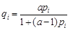
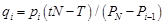
- Neufeld (2000) developed an alignment method that is a hybrid of Monte Carlo and the sidewalk method. DYNACAN adopted this approach with non-linear adjustment to the equation-generated probabilities, combined with a minor tweaking of the resulting probabilities depending on whether the simulated rate is ahead of or behind the target rate for the pool during the progress and some randomisations (Morrison 2006). The method calibrates the probabilities through nonlinear transformation instead of using predicted probabilities directly in order to confine the probability within the range of 0 and 1 (SOA 1998). Two parameters η and λ control the maximum difference allowed before the adjustment occurs, and the strength of the adjustment when the simulated probabilities deviates from the expectations. The method reduces the variance in the simulation by introducing a correlation between neighbouring observations. This, however, may not be an ideal property for a pure alignment exercise. Therefore, the implementation in this paper randomised the order of the observation before running the alignment to remove the correlation.
Algorithm 2: Sidewalk with Nonlinear Transformation
Input: pi (predicted probability obtained from the model for each observation i), t (target probability), N (total number of observations), η (maximum difference allowed, 0.5 in the original paper), λ (adjustment factor, 0.03 in the original paper)
Output: yi (simulated transition outcome)
Pseudo Code:
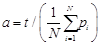
Find α so that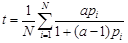
Randomize the order of observations
T = 0 (counter)
for i = 1 to N:
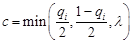
if then c = -c
r ← a random number from uniform distribution (0,1)
if (r+c) < qi then yi = 1 else yi = 0
T = T + yi
restore the observation orderThe Central Limit Theorem approach
- 3.6
- The Central Limit Theorem approach is described in Morrison (2006). It utilises the assumption that the mean simulated probability is close to the expected mean when N is large. It manipulates the probabilities of each individual observation on the fly so that the simulated mean matches the expectation. A more detailed description of the method can be found in Morrison (2006). Like all the methods we have discussed so far, this method does not need any sorting routine.
Algorithm 3: Central Limit Theorem Approach
Input: pi (predicted probability obtained from the model for each observation i), t (target probability), N (total number of observations)
Output: yi (simulated transition outcome)
Pseudo Code:
T = 0 (counter)

for i = 1 to N:
r ← a random number from uniform distribution (0,1)
if pi > r then
yi = 1
T = T + yi
else
yi = 0Sort by predicted probability (SBP)
- 3.7
- O'Donoghue (2001) and Johnson (2001) first documented sorting based alignment algorithms. This type of algorithm involves sorting of the predicted probability adjusted with a stochastic component, and selects desired number of events according to the sorting order. It is seen as a more "transparent" method (O'Donoghue 2010) although can be computationally more intensive due to the sorting procedure. Many variations of the methods have been used in the past years. In this paper, we discuss the commonly used variations: sort by predicted probability (SBP), Sort by the difference between predicted probability and random number (SBD), and Sort by the difference between logistic adjusted predicted probability and random number (SBDL).
- 3.8
- Sorting by probability method essentially picks up the observations with highest transition probabilities in each alignment pool. One consequence, however, is that those with the highest risk are always being selected for transition. In the example of employment, it is almost certain that higher educated will always be selected to have a job. In reality, those with the highest risk will on average be selected more than those with lower risk, but not always be selected. As a result some variability needs to be introduced. Kelly and Percival (2009) propose a variant of this method, where a proportion (typically 10% of the desired number) are selected when the sorting order is inverted, so as to allow low risk units to make a transition.
Algorithm 4: Sort by Probability
Input: pi (predicted probability obtained from the model for each observation i), t (target probability), N (total number of observations)
Output: yi (simulated transition outcome)
Pseudo Code:
sort by pi from largest to smallest (assume the new index is j)
if j ≤ Nt then yj = 1 else yj = 0
restore observation orderSort by the difference between predicted probability and random number (SBD)
- 3.9
- Given the shortcoming of the simple probability sorting, Baekgaard (2002) uses another method, which sorts by differences between predicted probability and a random number. Instead of sorting the predicted probability directly, it sorts a particular transformation qi, which equals the difference between predicted probability pi and a random number ri, a number that is drawn from a uniform distribution in range 0 to 1. Mathematically, this sorting variable qi can be defined as follows:
A concern about this method is that the range of possible sorting values is not the same for each point. In other words, because the random number ri∈[0,1] is subtracted from the deterministically predicted pi, the sorting value takes the range qi∈[-1,1]. However, for each individual qi will only take a possible range [ri-1, ri]. As a result, when pi is small say 0.1, the range of possible sorting values is [-0.9, 0.1]. At the other extreme if pi is large say = 0.9, then the range of possible sorting values is [-0.1, 0.9]. Thus because there is only a small overlap for these extreme points, an individual with a small pi will have a very low chance of being selected even if a low value random number is paired with the observation.
Algorithm 5: Sort by the difference between predicted probability and random number (SBD)
Input: pi (predicted probability obtained from the model for each observation i), t (target probability), N (total number of observations)
Output: yi (simulated transition outcome)
Pseudo Code:
for each observation i:
ri ← a random number from uniform distribution (0,1)
qi = pi - ri
sort by qi from largest to smallest (assume the new index is j)
if j ≤ Nt then yj = 1 else yj = 0
restore observation orderSort by the difference between logistic adjusted predicted probability and random number (SBDL)
- 3.10
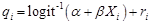
- An alternative method described in Flood et al. (2005), Morrison (2006) and O'Donoghue et al. (2009) mitigates the range problem of SBD by using logistic transformation. This method takes a predicted logistic variable from a logit model, logit(pi) = α + βXi combined with a random number ri that is drawn from a logistic distribution to produce a randomised variable. The sorting variable qi can therefore be described as follows:
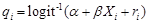
ri is a logistically distributed with mean value 0 and a standard error of
 . Since the random number is not uniformly distributed as ri in the previous method, it produces a different sorting order.
Algorithm 6: Sort by the difference between logistic adjusted predicted probability and random number (SBDL)
Input: pi (predicted probability obtained from the model for each observation i), t (target probability), N (total number of observations)
Output: yi (simulated transition outcome)
Pseudo Code:
for each observation i:
ri ← a random number from uniform distribution (0,1)
sort by qi from largest to smallest (assume the new index is j)
if j ≤ Nt then yj = 1 else yj = 0
restore observation order
Theoretical properties of Binary Alignment Methods
- 4.1
- While the computation complexity of each algorithm may be different, they all impose some implicit assumptions on the distribution. This section analyses the assumptions and discusses how the probabilities are changed from a theoretical point of view.
- 4.2
- The implicit assumption behind multiplicative scaling method is that all probabilities should be scaled up or down at the same time by the same proportional amount. However, since the probability is always bounded between 0 and 1, the distribution is likely to be distorted at high probability area.
- 4.3
- Sidewalk method is relatively complicated when used for alignment purpose. However, the probability changes can be estimated using a non-linear adjustment at the beginning of the algorithm. Since it adjusts the constant term of a logistic equation, the probability will change differently according to its original value. Probabilities around 0.5 will be most likely affected while the probabilities near 0 or 1 will be hardly changed. In another word, it assumes the shock on the exogenous target change is mostly absorbed by the observations in the middle of the probability spectrum.
- 4.4
- Central Limit Theorem approach has a relatively complicated transformation from a theoretical point of view. It has some similarities to multiplicative scaling method as it also uses scaling ratio but the ratio is constantly changing when the algorithm is running. The probability change would be dependent on both original value and the sequential position in the dataset.
- 4.5
- SBP algorithm does not pay much attention to the distribution. Instead, it selects individuals that are most likely to have the transitions. In this way, it may minimise the false positive or false negative. However, the distribution can be distorted since it is completely ignored in the calculation.
- 4.6
- While SBD imposes a uniformly distributed random number for all observations regardless of probabilities, its transformation is more complicated from a theoretical point of view. Compared with SBP, it allows lower probability observations to be selected. However, the aligned probability of an outcome varies in a nonlinear way from its original unaligned probability. For instance, if we need to select one observation in a sample of two observations with probability 0.1 for observation a and 0.9 for observation b, SBP method would always pick observation b, whereas in the case of SBD the observation a would be selected when 0.1+r1 > 0.9+r2 (where r1 , r2 are two i.i.d. random numbers with uniform distribution between 0 and 1) which has a probability of 0.04. The selection clearly favours the large probability observations but with less distortions compared with SBP.
- 4.7
- SBDL is based on an assumed logistic equation. Instead of changing the probability directly, it changes the constant term of the equation. Statistically, the probability transformation is similar to the nonlinear adjustment part of the Sidewalk method. The approach also shares similar statistical properties with the method of using a trend parameter used in the estimation, which is sometimes used as an ex ante approach for simulation alignment.
Methods of Evaluating Alignment Algorithm
- 5.1
- In order to evaluate the simulation properties of all alignment algorithms, it is important to define what we need to compare, and what the criteria are. Although different alignment methods have been briefly documented in a few papers, there is little discussion on the actual performance differences among these methods. Implementations vary from model to model, but no paper so far validates the alignment methods. This paper tries to evaluate different algorithms and compares how they perform under different scenarios.
Objectives of Alignment
- 5.2
- The objectives of alignment, discussed in Morrison (2006) and O'Donoghue (2010) serve as the basis of our evaluation criteria. From a practical point of view, a "good" alignment algorithm should be able to
- Replicate as close as possible the external control totals for the alignment totals. This is one of the main reasons why alignment is implemented in microsimulation and the common goal of all alignment methods as discussed in virtually all alignment papers, e.g. Neufeld (2000), Morrison (2006)
- Retain the relationship between the deterministic and explanatory variables in the deterministic component of the model (O'Donoghue 2010). In achieving the external totals, the alignment process should not bias the underlying relationship between the dependent and explanatory variables.
- Retain the shape of distributions in different subgroup and inter-relations unless there is a reason not to. Morrison (2006) suggests that alignment is about implementing the right numbers of events in the right proportions for a pool's prospective events, as opposed to simply getting the right expected numbers of events. Although alignment processes focus on the aggregated output, it should not significantly distort the relative distribution within different sub-groups. For instance, if we want to align the number of people in work, we not only want to get the numbers right at the aggregate level, but also at the micro/meso level, e.g. the labour participation rate for 30 years old should be higher than the rate for the 80 years old. This relative distribution should not be changed, at least substantially, by the alignment method. A highly distorted alignment process would adversely affect the distributional analysis, a typical usage of microsimulation models.
- Compute efficiently. There is no doubt that today's computing resources are much more abundant than before. However, when handling large dataset, e.g. full population dataset, computational constraint is still an important issue. Some projects, e.g. LIAM2/MiDaL (de Menten 2011), redesign the entire framework in order to achieve faster speed and accommodate larger datasets.
Indicators of alignment performance
- 5.3
- In order to assess the alignment algorithms with very different designs, the paper uses a set of quantitative indicators that can measure the simulation properties according to the criteria discussed earlier. The indicators include
- A general fit measure: false positive rate and false negative rate of the prediction, which reflect how well the final output fits the actual data in general.
- A target deviation index (TDI), which measures the difference between the external control and the simulation outcome. This indicator is directly linked to the first criterion.
- A distribution deviation index (DDI), which measures the distortion of the relationship between different variables and inter-relations, as discussed in criteria two and three.
- and a computational efficiency measurement: The number of seconds it takes to execute one round of alignment, including the overhead cost (e.g. sorting), as outlined in criterion four.
Target Deviation Index (TDI)
- 5.4
- Assuming among N observations, the ideal alignment ratio is t and the final binary output after alignment for observation i is yi. Target deviation index (TDI) is defined as
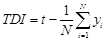
It is a percentage number ranged 0 to 1, and shows how the alignment replicates the external control. Higher values imply the outcome is further away from the external control. TDI is a simple index that examines the simulation output at aggregate value, one of the main purposes of alignment. However, it does not consider the internal distributions or false positive/negatives, which means other measurements are also needed to get an accurate picture of an alignment algorithm.
Distribution Deviation Index (DDI)
- 5.5
- In order to evaluate the second and the third criteria, it is necessary to find an indicator that can reflect how well the relationships are preserved and how different the new distribution is from the old one.
- 5.6
- One method is to compare the original coefficients with re-estimated coefficients from aligned data. Statistically identical coefficients indicate that the relationship remains the same, at least mathematically. However, this might not be applied to alignment tests, as alignment itself by definition, distorts the original probabilities. The coefficients, as a result, are bound to change even under an optimal alignment method, and in most cases, the "correct" aligned coefficients are not available.
- 5.7
- Another method to compare the relationships is to see whether the distribution of key variables have changed after alignment, e.g. whether the proportion of male workers and females workers have changed substantially. A Chi-square test could be useful for this scenario, as it is frequently used to test whether the observed distribution follows the theoretical distribution. Nevertheless, the test itself is not designed for binary values and requires "no more than 20% of the expected counts to be less than 5 and all individual expected counts are 1 or greater" (Yates et al. 1999& McCabe 1999). This requirement might not be always fulfilled in microsimulation depending on the scenario assumptions and the way groups are defined. As a result, an adaptation is required in order to best measure the deviation between two distributions for the purpose of binary variables and possibly low or zero expected counts.
- 5.8
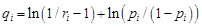
- This paper uses a self-defined distribution deviation index (DDI) to evaluate the second and third criteria in choosing an alignment method. Assuming we are going to evaluate the distribution distortion in a single alignment pool via a grouping variable X. X could be anything like age group, gender, or age group gender interaction etc. N observations of variable X can therefore be divided into n(X) groups with Nj observations in group j. If we define t as the external target ratio for alignment, yj,i as the binary output for observation i in group j after alignment and pj,i as the original probability for observation i in group j before alignment. A distribution deviation index (DDI), therefore, can be defined as
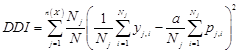
where
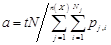
α is the ratio between exogenous total target and total accumulated probability in the dataset before alignment. The DDI indicator describes how well the micro-simulated data retain the relationships between dependent variable and variable X. Essentially, DDI calculates the sum of squares of differences weighted by the number of observations. It measures the differences between distributions before and after alignment in multiple dimensions, depending on the vector X. When X is an independent variable, it measures the distortion introduced between the independent variable and the dependent by alignment. The indicator is positively correlated with the alignment deviation. It increases when the aligned distribution departs from the original and decreases when the distributions become more alike. DDI has a range of 0 to 1. When the dataset preserves the shape of distribution perfectly, the index has a value of zero. It increases when the difference of two redistributions grows, with a maximum value of one.
Computation efficiency
- 5.9
- The most intuitive indicator for the computational efficiency of an alignment algorithm is the total execution time: the length of time an alignment method takes to execute one round of alignment with a given input dataset, including all the overhead costs of the algorithm, e.g. sorting, randomisations etc. In order to have comparable inputs and outputs, the evaluation in this paper requires all methods to retain the initial order of inputs. This makes the algorithm ready as a module in the microsimulation model. However, this extra requirement penalizes the speed of the methods that require randomly shuffling, as the observations need to be re-sorted before the end of the execution.
- 5.10
- The evaluation of the computational efficiency is performed in Stata because of its popularity in economic research and easy integration of estimation and simulation. The CPU time reported includes the algorithm time costs and the overhead time incurred. Given that the computer speed varies much, the results presented in this paper may change dramatically on a different platform although we would expect the relative ranking to remain stable in similar scenarios.
Alignment algorithms evaluated
- 5.11
- This paper evaluates all alignment algorithms discussed earlier, which includes,
- Multiplicative scaling
- Sidewalk Hybrid with Nonlinear Adjustment
- Central Limit Theorem Approach
- Sort by predicted probability (SBP)
- Sort by the difference between predicted probability and random number (SBD)
- Sort by the difference between logistic adjusted predicted probability and random number. (SBDL)
Datasets and Scenarios in Alignment Algorithm Evaluation
- 6.1
- In order to understand the simulation properties of alignment algorithms, this paper evaluates the performances of various methods using synthetic datasets. While real-world datasets can be used for evaluation, the complexity of the behaviour modelling in a dynamic microsimulation may overwhelm the analysis with the errors from sources other than alignment. Additionally, since we only observe the outcome variable rather than the probability in a real dataset, it is difficult to illustrate how probabilities are transformed under various alignment algorithms. Therefore, this paper uses a simple setting where the source of the error can be controlled.
- 6.2
- The paper tests the alignment performances of different models in four different scenarios. Each scenario represents a potential statistical error that alignment methods try to address or compensate for in a microsimulation model. The quality of the alignment is measured by the target deviation index (TDI), and the distribution deviation index (DDI), where the grouping variable X is the percentile of the correct probabilities. Computation cost is measured by the number of seconds the algorithm takes to execute one run.
Baseline scenario
- 6.3
- Assuming there is a binary model expressed as following
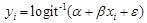
The independent variable x and the error term ε are drawn independently and randomly from a logistic distribution with mean zero and a variance of
. Compared with a standard normal distribution, using a logistic distribution for the independent variable will result in an evenly distributed true probability yi*, which makes it easier to compare the simulated probability and the true probability. To simplify the calculation, we assign α = 0, β = 1 in the base scenario. The number of observations in the dataset is 100,000. Table 1 lists all the key statistics in the baseline scenario and Figure 1 illustrates the distribution of the baseline probabilities.
First scenario: Sample bias
- 6.4
- In the first scenario, we try to replicate an error that commonly exists in survey datasets: sample bias. Sample bias exists widely among survey datasets and it is most commonly corrected by the implementation of observation weights. Unbiased estimations of behaviour equations depend on accurate weights. Nonetheless, despite all efforts, survey datasets may still suffer from various sample bias, particularly the selection bias and the attrition bias in panel dataset, such as ECHP (Vandecasteele and Debels 2007). Sample bias leads to a non-representative dataset, which affects the quality of simulation output. Alignment is sometimes used to compensate for the sample bias.
- 6.5
- In our test, a simple sample bias is recreated. We remove 50% of the observations with positive response (yi* > 0) randomly from the baseline dataset. This produces a non-representative sample with the size equivalent to 75% of the original one. In other words, the observations with non-positive response (yi* ≤ 0) weigh twice as much as they should in the dataset. In addition, the error structure (εi) has a different distribution than the baseline scenario as a consequence of the bias introduced.
Second scenario: Biased alpha (intercept)
- 6.6
- The second scenario aims to replicate a monotonic shift of the probabilities. This is commonly used in scenario analysis, where a certain ratio, e.g. unemployment rate, is required to be increased or decreased to meet the scenario assumptions.
- 6.7
- By manipulating the intercept of the equations, it is possible to shift the probabilities across all observations. In this scenario, α is changed to -1 while everything else is constant. The result is a monotonic, but non-uniform change in the probabilities. Contrary to the previous scenario, the error structure and the number of observations stay the same in this setup. Table 1 highlights the statistical differences between this scenario and the other ones.
Third scenario: Biased beta
- 6.8
- The third scenario introduces a biased slope β in the equation. This represents a change in the behaviour pattern which could not be captured at the time of estimation (e.g. the evolution of fertility pattern). In this scenario, one may assume that the behaviour pattern shifts over time. This particular setup tests how alignment works as a correction mechanism for changes in behaviour pattern.
- 6.9
- The simulated dataset in this scenario is generated with β = 0.5, half of its value in the baseline, and therefore creates a different distribution of probabilities. Since x has a mean value of 0, the change does not affect the total sample mean of y at the aggregate level. The transformation yields a different distribution but with an unchanged sample mean. The standard deviation of probabilities in scenario 3 is lower than the baseline scenario while the mean value remains the same.
- 6.10
- Unlike the first and second scenarios, the transformation in this scenario causes a non-monotonic change in probabilities. Observations with low probability (p < 0.5) in the baseline scenario have increased probability, while the observations with high probability (p > 0.5) have a lower probabilities compared with the baseline scenario.
Fourth scenario: Biased intercept and beta
- 6.11
- The last scenario combines both the change in intercept and the shift in slope. The new transformed dataset has an α = 1 and β = 0.5. This scenario represents a relatively complex change. The change results in a lowered aggregate mean of y and a non-monotonic change in the individual probabilities.
Table 1: Overview of the Synthetic Data Scenarios Scenario Scenario Baseline 1 2 3 4 Number of observations in estimation 100,000 75,000 100,000 100,000 100,000 Number of observation in simulation 100,000 100,000 100,000 100,000 100,000 α 0.000 -0.693 -1.000 0.000 -1.000 β 1.000 1.000 1.000 0.500 0.500 Target Ratio for Alignment 0.500 0.500 0.500 0.500 N.B.: Coefficients are theoretical values. The actual estimation in scenario 1 might differ from this value slightly given the random numbers drawn. - 6.12
- As an overview, Table 1 summarise the changes of alpha and beta in different scenario and compares the key statistics. As seen, all scenarios have the same number of observation except the first one. The target for alignment (external value) is 0.5 across all scenarios. Figure 1 gives a visualised picture of probability distributions in the different scenarios. We see that all probability distributions, with the exception of baseline and third scenario, exhibit a right skewed pattern.
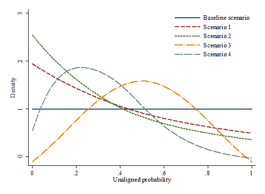
Figure 1. Overview of Probability Distribution in Different Scenarios
Evaluation Results
-
Properties of Various Alignment Methods in Simulation
- 7.1
- This section reports the evaluation results of six different alignment algorithms and compares their performances under different scenarios through false positive/negative rate, two self-defined indices (TDI, DDI) and computational time. To minimize the impact of random number drawing on the Monte Carlo exercise and to estimate the standard deviation of the reported values, each scenario has been simulated for 100 times. Table 2 reports the means values and the standard deviations of the simulation output. The DDI calculation uses the percentile of the corrected probabilities as the grouping variable.
Table 2: Prosperities of Different Alignment Methods using Synthetic Dataset Method TDI (%) False Positive (%) False Negative (%) DDI (%) Mean S.D. Mean S.D. Mean S.D. Mean S.D. Scenario 1: Selection Bias Multiplicative scaling -1.810 (0.127) 14.656 (0.126) 16.466 (0.091) 0.428 (0.028) Sidewalk hybrid with nonlinear adjustment 0.000 (0.004) 16.608 (0.093) 16.608 (0.093) 0.033 (0.004) Central limit theorem approach -0.056 (0.013) 15.383 (0.096) 15.440 (0.094) 0.378 (0.018) Sorting (SBP) 0.000 (0.000) 12.505 (0.066) 12.505 (0.066) 8.125 (0.087) Sorting (SBD) 0.000 (0.000) 17.223 (0.096) 17.223 (0.096) 0.255 (0.018) Sorting (SBDL) 0.000 (0.000) 16.664 (0.095) 16.664 (0.095) 0.033 (0.005) Scenario 2: Biased Alpha (Intercept) Multiplicative scaling -3.287 (0.130) 13.709 (0.104) 16.996 (0.096) 0.892 (0.051) Sidewalk hybrid with nonlinear adjustment 0.001 (0.004) 16.612 (0.080) 16.611 (0.080) 0.033 (0.005) Central limit theorem approach -0.307 (0.030) 15.015 (0.086) 15.323 (0.080) 0.531 (0.020) Sorting (SBP) 0.000 (0.000) 12.505 (0.066) 12.505 (0.066) 8.125 (0.087) Sorting (SBD) 0.000 (0.000) 17.702 (0.093) 17.702 (0.093) 0.493 (0.025) Sorting (SBDL) 0.000 (0.000) 16.680 (0.086) 16.680 (0.086) 0.032 (0.005) Scenario 3: Biased beta coefficient Multiplicative scaling -0.009 (0.147) 19.640 (0.127) 19.649 (0.114) 1.178 (0.044) Sidewalk hybrid with nonlinear adjustment 0.000 (0.005) 19.587 (0.090) 19.586 (0.091) 1.146 (0.043) Central limit theorem approach 0.000 (0.000) 19.636 (0.100) 19.636 (0.100) 1.175 (0.042) Sorting (SBP) 0.000 (0.000) 12.505 (0.066) 12.505 (0.066) 8.125 (0.087) Sorting (SBD) 0.000 (0.000) 19.629 (0.088) 19.629 (0.088) 1.175 (0.043) Sorting (SBDL) 0.000 (0.000) 19.638 (0.095) 19.638 (0.095) 1.176 (0.042) Scenario 4: Biased alpha and beta (all coefficients) Multiplicative scaling -1.062 (0.133) 17.327 (0.117) 18.389 (0.098) 0.522 (0.036) Sidewalk hybrid with nonlinear adjustment 0.000 (0.005) 19.599 (0.077) 19.599 (0.077) 1.151 (0.038) Central limit theorem approach -0.001 (0.002) 17.772 (0.090) 17.773 (0.090) 0.369 (0.022) Sorting (SBP) 0.000 (0.000) 12.505 (0.066) 12.505 (0.066) 8.125 (0.087) Sorting (SBD) 0.000 (0.000) 20.477 (0.079) 20.477 (0.079) 1.991 (0.053) Sorting (SBDL) 0.000 (0.000) 19.632 (0.095) 19.632 (0.095) 1.178 (0.041) Note: Mean and standard deviations are calculated based on 100 independent simulations with 100,000 observations in each repetition. - 7.2
- As seen in Table 2, all alignment methods except multiplicative scaling, in all scenarios, have less than 0.5% deviation from the target number of event occurrence while multiplicative scaling shows a deviation of 0–3% from the target on average. The result is largely driven by the design of the algorithm, as multiplicative scaling cannot guarantee a perfect alignment ratio although the expected deviation is zero. Sidewalk hybrid sometimes has a slight deviation, as the non-linear transformation may not be always perfect under existing implementation[2]. Central limit theorem methods have built-in counters that prevent the events from manifesting when the target is met, so it tends to score a small negative ratio in target deviation index (TDI). Sorting based algorithms only pick the exact number of observations required, which is why their TDIs are always zero.
- 7.3
- In terms of false positive and false negative rates when compared with the "correct" values, alignment method SBP yields the best result, which is on average 4 to 6 percentage points lower than other algorithms, as shown in the tables. Sidewalk Hybrid, together with SBD, SBDL, have the highest false positive/ false negative rates on average. It seems that the false positive and false negative rates are closely related to the complexity of the algorithms. The "nonlinear transformation" in Sidewalk Hybrid and "differencing" operations in SBD and SBDL are both more computationally complicated than the other methods. This pattern is consistent across all scenarios, though absolute numbers fluctuate across different scenarios.
- 7.4
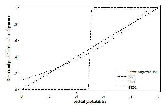
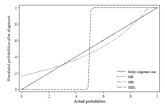
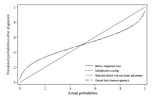
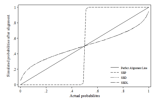
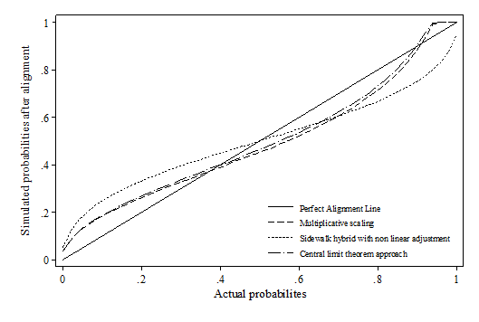
- Whilst false positive and false negative is a useful indicator when the correct value is known, it is a less critical indicator for simulation as microsimulation exercises tend to focus more on the distributions. Therefore, the distribution deviation index (DDI) is particularly important in judging how well the relative relations between variables are preserved after alignment. Appendix 1 visualises the difference between actual probabilities and aligned probabilities.
- 7.5
- The results show that the SBP method heavily distorts the original distribution of the probabilities across all scenarios using percentile grouping. This is also reflected by the distributional deviation index (DDI), which is effectively calculating a weighted size of the gap in this case. It seems that there is no method consistently outperforming across all scenarios. In the first two scenarios, sidewalk hybrid and SBDL methods give the best result; In the third scenario, where the synthetic dataset modifies the slope of xi, all methods have similar DDI values except SBP; In the last scenario, multiplicative scaling and central limit methods generally perform much better than the rest. Compared with other methods, methods which involves "differencing" and "logistic transformation" (incl. sidewalk hybrid with non-linear transformation, SBD and SBDL) seem to be more sensitive to the change in the beta coefficient. Their performances are much better when beta remains stable, e.g. scenario 1 and 2. This may be due to the nature of these algorithms as the "differencing" and "logit transformation" operations assume monotonic changes in the probabilities.
Computing Performance
- 7.6
- Computational efficiency is another main criterion for evaluating alignment algorithm. Given the increasing availability of large-scale datasets in microsimulation and the growing model complexity, alignment may consume considerable resources in the computation processes. Table 3 shows an overview of the computation time required. The computational premium is timed on an Intel Xeon E5640 processor with only single core used for calculation. As indicated, the method that takes least computation resources is multiplicative scaling method. This is not surprising, as multiplicative scaling involves only a single calculation for each observation. Sorting-based alignment methods seem to be in the next tier, consuming up to 5 times more resources compared with multiplicative scaling. The variations in sorting method do not change the execution time much although the last sorting variation, SBDL, consumes slightly higher resources on average, although the time needed are not significantly different base on 100 rounds of simulations.
- 7.7
- Sidewalk Hybrid with nonlinear transformation seems to be on the bottom list in terms of the efficiency. It takes almost 100 times more CPU time than that required by the fastest method, multiplicative scaling. There are three reasons for its relatively poor performances. Firstly, the nonlinear transformation may take many iterations and it is computationally expensive (Neufeld 2000). Secondly, the method itself suffers from serial correlation in the original design, as the calculation is dependent on the result of the last observation. In order to mitigate this effect, an extra randomisation via sorting is implemented. This is accompanied by a reverse process, which restores the original order of the input at the end of the alignment. Thirdly, the Sidewalk method requires iterating through observations. Stata, which is the platform of our evaluation, is not particularly efficient at individual observation iteration compared with the vector based processing for which Stata optimises[3]. This is also the primary reason why Central limit theorem approach has a relatively long running time. We speculate from a theoretical point of view, that the performances of the Sidewalk method and the Central limit theorem approach could be significantly improved when implemented correctly as native code in C/C++ as compiled code does not re-interpret the syntax over the iterations. Nonetheless, the sidewalk method may still be slower than the other algorithms when nonlinear probability transformation is applied.
Table 3: Computational Costs for Different Alignment Methods Computation Time
(milliseconds for 100,000 observations)Scenario 1 Scenario 2 Mean S.D. Mean S.D. Multiplicative scaling 49.85 (10.19) 51.49 (10.12) Sidewalk hybrid with nonlinear adjustment 5359.30 (195.06) 5547.86 (195.06) Central limit theorem approach 3121.28 (164.03) 3243.07 (164.03) Sorting (SBP) 169.78 (19.78) 171.58 (19.78) Sorting (SBD) 180.01 (24.34) 178.53 (24.13) Sorting (SBDL) 193.29 (17.96) 199.02 (24.83) Scenario 3 Scenario 4 Mean S.D. Mean S.D. Multiplicative scaling 50.24 (9.77) 50.05 (10.62) Sidewalk hybrid with nonlinear adjustment 5192.32 (195.06) 5467.01 (195.06) Central limit theorem approach 3345.88 (164.03) 3735.48 (164.03) Sorting (SBP) 170.00 (19.78) 170.87 (19.78) Sorting (SBD) 179.26 (25.25) 178.06 (22.11) Sorting (SBDL) 197.44 (25.58) 194.27 (24.75) N.B. Mean value and standard deviations are calculated based on 100 rounds of simulations. Results are obtained on Intel Xeon E5640 CPU with Stata 11 SE Windows version using Stata's internal timer. - 7.8
- Due to the actual implementation will vary in different environments, the results do not reflect the performance in real projects on a different platform, but do provide a reference to illustrate the potential computation cost. It is important to note that since the sorting algorithm and most calculations are encapsulated in Stata, the actual performance is the mixed result of Stata memory management, calculation performance, algorithm design quality, and implementations. The actual performance may be very different in other implementation settings (e.g. C/C++).
Conclusion
- 8.1
- Alignment is often used as a last resort pragmatic solution to impose exogenous restrictions into the simulation process. Microsimulation models uses alignment for various purposes, e.g. historical data alignment in CORSIM, forecasting alignment in APPSIM etc. While it may not be elegant, it is de facto widely adopted over the past decade in the field of microsimulation. However, there is a lack of review of the alignment method implementations. This paper fills a gap in the literature in relation to the evaluation of different alignment algorithms. Although pervious literatures, e.g. Johnson (2001), Morrison (2006), and O'Donoghue (2010) have listed a few criteria that a "good" alignment method should meet, and analysed some theoretical expectation of the alignment simulation properties and their performances, e.g. Morrison (2006), there was no direct or quantitative comparison of various methods.
- 8.2
- In this paper, we have reviewed and evaluated most binary model alignment techniques, including multiplicative scaling, hybrid sidewalk method, central limit theorem approach and sorting based algorithms (including its variations). The paper compares different algorithms through a set of indicators including false positive rate, false negative rate, self-defined target deviation index (TDI), distribution deviation index (DDI), and computation time. Target deviation index (TDI), gives a scale independent view on how well an alignment method replicates the external control. The false positive, false negative rate, give an overview on the general quality of the output after alignment. The preservation of inter-correlations is measured by the distribution deviation index (DDI), an indicator ranged 0 to 1. It calculates the distance between the ideal distribution and the actual distributions after the alignment.
- 8.3
- The evaluations report a mixed result of alignment performances. It shows that the selecting the "best" alignment method is not only about the algorithm design, but also the requirements and reasoning in a particular scenario.
- 8.4
- Overall speaking, multiplicative scaling is the easiest to implement, and fastest to compute method for alignment. It could align more than millions of observation in a fraction of seconds in a mainstream computer at the time of writing. Nonetheless, it cannot perfectly align to external control as the events are calculated purely based on the calculated probabilities. Moreover, due to lack of restrictions in the algorithm design, the outcome produced by the multiplicative scaling method is subject to higher fluctuations than by other methods. Sidewalk hybrid with nonlinear adjustment is a computationally expensive method due to its nonlinear adjustment. However, the method has an above average performance in all scenarios. It exhibits a similar pattern with one sorting based method, sort by the difference between logistic adjusted predicted probability and random number (SBDL). Because of the logistic transformation applied in both algorithms, both methods are good at handling the error of intercept in logit model. Central limit theorem approach tends to have similar statistical patterns with multiplicative scaling method except it can match the alignment target more precisely. Nonetheless, the algorithm is very slow when implemented in Stata due to the need of iterating observations.
- 8.5
- As to the sorting based algorithms, the sort by probabilities (SBP) method yields the best result in terms of false positive and false negative whilst it distorts the internal distributions heavily in most cases. This is due to the nature of the algorithm, which over-predicts the observations with higher probabilities and under-predicts the observations with lower probabilities. However, the method is easy to implement and does not involve random number sorting. Its simulation properties suggest that SBP is a good method in imputation, but not ideal for forward or backward simulation. Sort by the difference between predicted probability and random number (SBD) and Sort by the difference between logistic adjusted predicted probability and random number (SBDL) are similar in terms of computation steps, but they produce very different distributions of probability. SBDL works better with logit model, especially when the intercept is used for alignment calibration. SBD seems to have below average performances when looking at all indicators and scenarios.
- 8.6
- As the results show, the selection of alignment methods is more complicated than previously thought. Each algorithm has its own advantages and disadvantages. For a microsimulation project focuses heavily on speed, multiplicative scaling seems to be a good choice. Central limit theorem approach could also be considered when implemented in a compiled language, like C/C++. In a project where speed is not the major concern, the choice might depend on the reason for alignment. For instance, if alignment is used to create a shift in intercept, SBDL or sidewalk hybrid with nonlinear transformation may be the best choice. In addition, for microsimulation analysis with the focus on distributional analysis, SBP may not be the ideal because of its distortion of distributions.
- 8.7
- Understanding the simulation properties is not an easy task as there are many implicit and explicit assumptions in every simulation project. The evaluation method used in this paper also has its own limits as it only covers some common errors and simulation scenarios in the test. However, the sources of errors in a real simulation are more complex than what has been illustrated and the assumptions on the distribution of independent variables may not always hold.
- 8.8
- Future research may look into the statistical properties of these alignment methods in real-world datasets, especially to compare the aligned simulation distribution with the actual data collected. As different alignment methods impose different assumptions, assessing the statistical impact when these assumptions are violated in real world simulations can be very useful. This would help us to choose the most appropriate method in simulating common social economic attributes. Additionally, it is also important to explore other options of incorporating external information into microsimulation and evaluate whether the constrained estimation approach can be a better alternative to simulate policy reforms than the current ex post alignment techniques.
Notes
-
1It is possible to incorporate the external information into the estimation, which forms a constrained estimation problem. An example of this used in microsimulation can be found in Klevemarken (2002). The method would eliminate the need for ex post alignment. However, estimating all equations with potential external constraints and allowing the possible correlations in the error terms could make both the baseline estimations and the simulations computationally challenging.
2The process usually requires several iterations and it is computationally expensive (Neufeld 2000). Our test model used in this paper stops its calibration when the iteration only improves the average probability by no more than 10-8. This increases the calculation speed but sometimes results in imperfectly aligned probabilities. Details of the calibration steps can be found in the book published by Society of Actuaries (SOA 1998).
3Observation iteration, a necessary step for these two algorithms, tends to be very slow in Stata because loops are reinterpreted at each iteration. Stata recommends using compiled plug-in for the best performance for this type of scenarios (Stata 2008). However, algorithm specific optimization using compiled code is beyond the scope of this paper and it would make the comparison difficult.
References
-
ANDERSON, J. M. (1990). Micro-macro linkages in economic models. In G. H. Lewis & R. C. Michel (Eds.), Microsimulation techniques for tax and transfer analysis. Urban Institute, Washington, DC.
BACON, B., & Pennec, S. (2009). Microsimulation, Macrosimulation : model validation, linkage and alignment. Paper presented at the 2nd General Conference of the International Microsimulation Association, Ottawa, Canada.
BAEKGAARD, H. (2002). Micro-macro linkage and the alignment of transition processes : some issues, techniques and examples. National Centre for Social and Economic Modelling (NATSEM) Technical paper No. 25.
CALDWELL, S., Favreault, M., Gantman, A., Gokhale, J., Johnson, T., & Kotlikoff, L. J. (1999). Social security's treatment of postwar Americans Tax Policy and the Economy, volume 13 (pp. 109–148): MIT Press.
CHENARD, D. (2000a). Individual alignment and group processing: an application to migration processes in DYNACAN. University of Cambridge. Department of Applied Economics.
CHÉNARD, D. (2000b). Earnings in DYNACAN: distribution alignment methodology. Paper presented at the 6th Nordic workshop on microsimulation, Copenhagen.
DAVIES, J. B. (2004). Microsimulation, CGE and macro modelling for transition and developing economies: WIDER Discussion Papers//World Institute for Development Economics (UNU-WIDER).
DE MENTEN, G., Dekkers, G., & Liégeois, P. (2011). LIAM 2: a new open source development tool for the development of discrete-time dynamic microsimulation models. Paper presented at the IMA Conference, Stockholm, Sweden.
DUNCAN, A., & Weeks, M. (1998). Simulating transitions using discrete choice models. Papers and Proceedings of the American Statistical Association, 106, 151–156.
FLOOD, L., Jansson, F., Pettersson, T., Pettersson, T., Sundberg, O., & Westerberg, A. (2005). SESIM III–a Swedish dynamic microsimulation model. Handbook of SESIM, Ministry of Finance, Stocholm.
JOHNSON, T. (2001). Nonlinear alignment by sorting: CORSIM Working Paper.
KELLY, S., & Percival, R. (2009). Longitudinal benchmarking and alignment of a dynamic microsimulation model. Paper presented at the IMA Conference Paper, Canada.
KLEVMARKEN, N. A. (2002). Statistical inference in micro-simulation models: incorporating external information. Mathematics and computers in simulation, 59(1), 255–265. [doi:10.1016/S0378-4754(01)00413-X]
LI, J., & O'Donoghue, C. (2012). Simulating Histories within Dynamic Microsimulation Models. International Journal of Microsimulation, 5(1), 52-76.
MORRISON, R. (2006). Make it so: Event alignment in dynamic microsimulation. DYNACAN paper.
NEUFELD, C. (2000). Alignment and variance reduction in DYNACAN. In A. Gupta & V. Kapur (Eds.), Microsimulation in Government Policy and Forecasting (pp. 361–382). Amsterdam: North-Holland.
O'DONOGHUE, C. (2001), “Redistribution in the Irish Tax-Benefit System”, PhD Thesis, London School of Economics, London.
O'DONOGHUE, C. (2010). Alignment and calibration in LIAM. In C. O'Donoghue (Ed.), Life-Cycle Microsimulation Modelling: Constructing and Using Dynamic Microsimulation Models.: LAP LAMBERT Academic Publishing.
O'DONOGHUE, C., Lennon, J., & Hynes, S. (2009). The Life-cycle Income Analysis Model (LIAM): a study of a flexible dynamic microsimulation modelling computing framework. International Journal of Microsimulation, 2(1), 16–31.
PEICHL, A. (2009). The benefits and problems of linking micro and macro models–Evidence from a flat tax analysis. Journal of Applied Economics, 12(2), 301–329. [doi:10.1016/S1514-0326(09)60017-9]
SCOTT, A. (2001). A computing strategy for SAGE: 1. Model options and constraints: Technical Note 2. London, ESRC-Sage Research Group.
SOA. (1997). Chapter 5 on CORSIM, from http://www.soa.org/files/pdf/Chapter_5.pdf
SOA. (1998). Chapter 6 on DYNACAN, from http://www.soa.org/files/pdf/Chapter_6.pdf
STATA. (2008). Creating and using Stata plugins, from http://www.stata.com/plugins/
VANDECASTEELE, L., & Debels, A. (2007). Attrition in panel data: the effectiveness of weighting. European Sociological Review, 23(1), 81–97. [doi:10.1093/esr/jcl021]
WINDER, N. (2000). Modelling within a thermodynamic framework: a footnote to Sanders (1999). Cybergeo: European Journal of Geography.
YATES, D. S., Moore, D. S., & & McCabe, G. P. (1999). The Practice of Statistics: Macmillan Higher Education.
Appendix 1 : Actual vs. Aligned Probabilities with Synthetic Datasets
-
Scenario 1: Sample bias
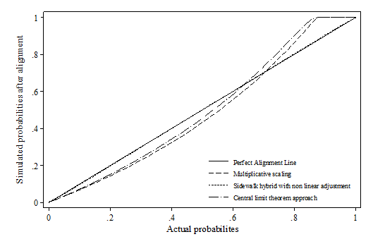
Abbreviations used in the Figure
SBP: Sort by predicted probability
SBD: Sort by the difference between predicted probability and random number
SBDL: Sort by the difference between logistic adjusted predicted probability and random number
Scenario 2: Biased Alpha (Intercept)

Abbreviations used in the Figure
SBP: Sort by predicted probability
SBD: Sort by the difference between predicted probability and random number
SBDL: Sort by the difference between logistic adjusted predicted probability and random numberScenario 3: Biased Slope (Beta)
Abbreviations used in the Figure
SBP: Sort by predicted probability
SBD: Sort by the difference between predicted probability and random number
SBDL: Sort by the difference between logistic adjusted predicted probability and random number
Scenario 4: All coefficients biased

Abbreviations used in the Figure
SBP: Sort by predicted probability
SBD: Sort by the difference between predicted probability and random number
SBDL: Sort by the difference between logistic adjusted predicted probability and random number