
 Abstract
- Although agent-based modeling is a strong modelling method in many aspects, its high degree of freedom in agent design can also be regarded as weakness. This freedom requires strong validation strategies during model design for empirical models, especially when models aim to be descriptive enough for policy support. Where theory or evidence does not support model design, assumptions are usually made. In these cases, arguments should be given for why the assumptions do not impair the validity of results. However, we believe that such justifications are sometimes weak in such kinds of models. In particular, we believe that the justification arguments are mostly plausible, but often not strong enough to overrule other plausible arguments leading to different designs. We believe that the reasons for this argumentative ambiguity are sometimes rooted in the type of underlying theory, framework, or validation strategy chosen. The point is that we suspect that simulation results can be sensitive to this ambiguity. To test this hypothesis, we selected a well-tried theory/framework/validation design strategy, and built alternative versions of a land-use change model in line with the underlying strategy. Results clearly show that levels and direction of simulated land-use change are significantly different among model versions.
- Keywords:
- Agent-Based Modelling, Policy-Support-Tool, Critique, Justification, Land Use
Introduction
- 1.1
- Although the many strengths of agent-based simulation have been emphasized frequently in the recent decade, little has been written so far on one of its weaknesses - its flexibility in agent design. At least in the field of land-use modeling, authors seem to agree that the freedom of the modeller in designing agents is not only a benefit, but can also be considered a weakness (Parker et al. 2001; Parker et al. 2003). This freedom combined with a frequent sparsity of available theory for agent design or choice of inappropriate design strategies often involves that modellers need to make assumptions in model design. When done in descriptive models, assumptions need to be justified, i.e. an argument needs to be given why the assumption does not impair the validity of results. However, we believe that such justification is sometimes weak in this respect. This may be rooted in the ambiguous nature of the underlying design strategy chosen, allowing several types of assumptions and associated justification. We suspect that models can be sensitive to this ambiguity. In particular, we suspect that this weakness can lead to contradicting simulation results and conclusions.
- 1.2
- Here, we test this hypothesis for the design strategy of the LUDAS (Land-Use DynAmic Simulator) model family, which was used to implement several models world-wide, i.e. VN-LUDAS (Vietnam) by Le et al. (2008), GH-LUDAS (Ghana) by Schindler (2010), SRL-LUDAS (Sri Lanka) by Kaplan (2011), LB-LUDAS (Lubuk Beringin, Indonesia) by Villamor (2012), and IM-LUDAS (Inner Mongolia, China) by Miyasaka et al. (2012). Projects for Burkina Faso and South Korea are ongoing. For this article, we analyzed the (joint) design strategy of this model family, originating from the first publication by Le (2005). To test our hypothesis, we selected an improved version of the GH-LUDAS model, analyzed what other designs the design strategy would allow, implemented these alternatives, and compared simulation results. Results clearly show significantly contradicting land-use trends among versions, both in magnitude and direction.
- 1.3
- In section 2, we outline the analysis of the LUDAS design strategy, including the LUDAS conceptual framework, provide a detailed description of GH-LUDAS, and present an alternative design for three selected model parts each. Thereby, the model design and its alternatives are in accordance with the design strategy. In section 3, we conduct simulations for all eight combinations of designs, and analyze results. Finally, we discuss results and what we believe this means for validation and design strategy choice.
Methods and materials
-
LUDAS: Design strategy and framework
Design strategy
- 2.1
- Agent-based models are models that are built from the specifications of entities called agents, including their actions and interrelations. The purpose of agent-based modelling is thus to simulate the behavior of the system that emerges from these specifications, being a non-linear phenomenon due to the implemented interconnectivity of agents. With regard to land use, agents usually include two main categories of agents, i.e. land patches, and land users situated on these land patches and being able to modify them. Consequently, most agent-based land-use change models are built on such a conceptual framework. That is, human agents are coupled with their environment through land-use choices and ecological returns. Land-use change patterns then emerge from this feedback loop.
- 2.2
- The core of the LUDAS design strategy is the LUDAS conceptual framework, which implements this idea and extends it. In particular, it is centered around the argument that heterogeneity and dynamics of household livelihood are central to (gradual) land-use change. The theoretical background of this argument has been outlined by Ellis (2000) and Le et al. (2008). In particular, Ellis argues that a household's livelihood influenced its survival strategy (Ellis 2000), which implies that land-use choices are influenced by the livelihoods of rural household agents. In addition, Le et al. (2008, p. 136, bottom) emphasize the importance of heterogeneity in triggering different agent behavior. The LUDAS framework incorporates both ideas through dynamic livelihood classes of household agents. Thereby, each livelihood class has an individual income and land-use strategy. The classes are dynamic in the sense that household agents need to change their class when livelihood assets have changed accordingly. This has consequences for resulting land-use choices. Subsequent ecological returns affect household livelihood assets. This process thus forms a secondary feedback loop at higher scale of analysis, in addition to the basic feedback loop described above. The components of both feedback loops are implemented via a set of interlinked sub-models (see 2.6). Particular statistical methods are associated with these sub-models.
- 2.3
- Here, we would like to note that the guidelines of the LUDAS design strategy were not well documented. For the subsequent LUDAS publications, this in particular embodied both the danger of flexibility in its application, but also the danger of mistaking it as theory that is easily transferable. However, the conceptual framework was adopted by all of the LUDAS models. In the majority of LUDAS publications, sub-models were added to the framework if required, for e.g. ecosystem service payments (Villamor 2012; Miyasaka et al. 2012), grazing (Schindler 2010; Miyasaka et al. 2012), or irrigation farming (Schindler 2010). The structural form of these sub-models was either adopted from theory (e.g. grazing in Schindler 2010), or was composed of statistical methods already employed in the LUDAS conceptual framework (e.g. multinomial/binary logistic regression, e.g. in ecosystem payment (Villamor 2012)). Justifications of the choice which components to add or which statistical tools to use for implementing them was sparse.
- 2.4
- In all cases, the design strategy for parameterization of the sub-models consisted of ethnographic methods. Little information regarding the specific employed strategy has been mentioned in the publications, but there is evidence that most of it is based on a collection of field notes and observation. However, the qualitative understanding of the study-area conditions seemed to be confined to supporting solely the choice of variable sets and to some extent the choice and design of additional sub-models. Household, plot, and/or GIS surveys were then conducted to collect and generate the required household and patch variables, completed by spatial map layers and other secondary data.
- 2.5
- In our case, the model framework was completed following field notes obtained from observation, expert opinion, transcripts of interviews, sample surveys, and published documents. The choice of candidates for explanatory variables and the algorithmic form of added sub-models were informed by the ethnographic analysis and by theory. The final parameterization and the calibration of sub-models, including land-use choice, was achieved via data from sample surveys and statistical analysis.
LUDAS framework
- 2.6
- In the LUDAS framework, household agents are represented by attributes and by an annual decision-making module. Landscape agents (square patches) are represented by attributes and ecological sub-models. The two types of agents are linked by tenure relations and feedback (for details see Le et al. 2008) (Figure 1). Policies may intervene in this coupled system by either changing household or environmental attributes, or their tenure relations, thus potentially changing system behavior. The basic feedback loop between household agents and patches takes the form of land-use choices and subsequent ecological returns affecting household livelihood assets and thus choices. This is implemented by household agents running a land-use choice phase, in which patches are selected for use, as long as the agent's labor budget is positive. In particular, the location, land-use type, and management mode of patches is selected. These choices depend on household characteristics and assets, environmental attributes, and the livelihood strategy. Crop return is finally calculated for each patch depending on these choices.
- 2.7
- During the land-use choice phase, patches that are assigned to the agent as owned are first cultivated. Then a search routine for rental land starts. The search for suitable patches to rent occurs within an aggregate of search radii, called the Landscape Vision. The evaluation of patches is achieved via comparison of utilities. These are calculated via multinomial or binary logistic regression models, whereby coefficients are specific to the livelihood class of the human agent. The choice among land-use types for a patch follows the ordered choice principle among utilities (Benenson and Torrens 2004). The mode of management is mostly modelled via assignment of constants (with or without uncertainty ranges), dependent on relevant policy, household or environmental variable values. Given these choices, ecological returns from patches are calculated. These are modelled by (a complex of) interacting ecological sub-models, including at least a crop production model. This crop production model calculates crop return dependent on the management decisions and natural factors for each land-use type. Aside from land-use returns also non-land-use related benefits are calculated, dependent on the livelihood class of the agent.
- 2.8
- After this basic feedback loop, model variables are updated. Given these updates, the most typical livelihood class is finally selected for the household. The livelihood classes are determined by applying Principle Component Analysis and k-mean Cluster Analysis to a range of explanatory variables using the widely used livelihood asset framework by Ashley and Carney (1999) (for details see Le 2005).
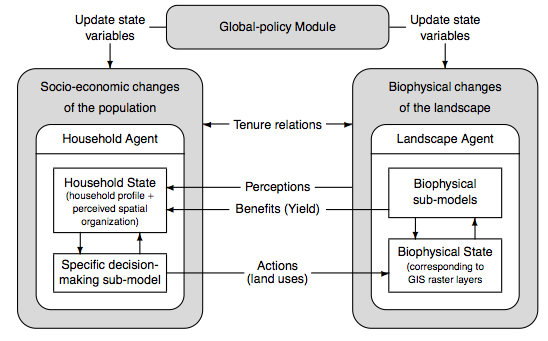
Figure 1. LUDAS framework: Basic feedback loop GH-LUDAS: Settings and data
Settings
- 2.9
- The study area comprises the Ghanaian part of the catchment of the Atankwidi, which is a tributary of the White Volta River, being located in the Upper East Region of Ghana with an area of 159 km2. Topography is rather flat to undulating, being interrupted by gullies extending from the widely branched riverbed. The majority of soils are lixisols, while leptosols are prevalent in the north east and fluvisols along the river side (Martin 2005). Climate is characterized by a rainy season lasting from May to October and a complementary dry season, whereat cultivation is largely limited to the rainy season, aside from some cash cropping activities via shallow groundwater irrigation in the dry season. High population density has transformed the area to a savannah parkland, being densely interspersed with singular farm compounds, farm and grazing patches, with little space for natural vegetation in the more highly populated areas. Rainfed cultivation is mainly meant for subsistence, comprising cultivation of millet varieties (Milium vernale, Pennisetum claucum), sorghum (Sorghum guineense), cowpeas (Vigna unguiculata), bambara beans (Vignea subterranea), groundnuts (Arachis hypogaea), rice (Oryza sativa), and kitchen vegetables, which can be categorized into three land-use types of cereal, groundnut, and rice, in reference to the main crop of the respective culture (Schindler 2010). Other household activities comprise livestock rearing, handicrafts, processing of agricultural products, trading, and non-farm activities such as teaching or farm wage laboring. As a compound usually houses an extended family with a complex land-use tenure and authority system, we defined a household as all people who are dependent on the person who decides about and manages a piece of land (for a detailed reasoning see Schindler 2010).
Data collection
- 2.10
- The presented model is grounded on data collected in 2006 in the study area for implementing an agent-based model of the local coupled human-environment system to study land-use change (Schindler 2010). In this context, two household surveys—one for each season—a ground-truth survey and a market survey were conducted. The household surveys were conducted among the same 200 households, which were spatially randomly sampled via GPS in the field, and comprised the collection of both household and plot data (for questionnaires see Schindler 2010). Household data comprised human, social, biophysical, land, and financial assets as well as access and impact of selected policies. Sizes of all household plots were recorded via GPS as well as their corresponding yields and inputs. In total, 814 plots were measured, and their yields were converted from local units to currency using price data and conversion tables from the market survey. In addition to literature review and field observation, an extensive series of informal farmer and expert interviews was used to identify relevant processes of system functioning and required data.
- 2.11
- Spatial data were collected during a ground-truth survey, which was used to classify an ASTER Satellite image via supervised classification for land-cover mapping, and from existing maps and models. Topographical data were derived from a Digital Elevation Model (DEM) by Le (2006), village borders were identified via landmarks and accordingly digitized, while all compound buildings in the study were identified through systematic raster search of a high-resolution Quickbird satellite image. Soil data were developed on the basis of Adu (1969) and Nunifu and Murchison (1999). Finally, all spatial data were converted to 30 × 30 m raster data to be identified with the agent-based grid of patches.
GH-LUDAS
- 2.12
- GH-LUDAS was developed following the design strategy as employed by the LUDAS models (see 2.2), and using the LUDAS conceptual framework as a core framework (see 2.6). Here, we would like to note that the conceptual framework is not consistently or clearly defined by Le (2005) or Le et al. (2008). For many parts of the original model by Le (2005), it is unclear whether they pertain to a generalizable and transferable framework, or whether they were designed specifically with respect to the Vietnamese case study. Some details of model, e.g. update of age or demographic variables, are insufficiently justified or lack justification; in many cases this suggests their transferability, in particular when either no reference is made to the case study, they explicitly draw on theory, or they lack explanation. It is also such kind of details that offer alternative designs through their ambiguity in justification. The model is available at http://www.openabm.org/model/3274.
Household agent
- 2.13
- According to Le (2005), the LUDAS conceptual framework involves the characterization of a household agent by a set of variables (Hprofile), a set of rules that update those variables that are not internally updated by other components of the model (FH-internal), a set of land patches whose information the agent can perceive for potential farmland extension (LandscapeVision), an embedded decision-making module (DECISION), and household behavioral parameters for the latter (Hbehavior).

(1) 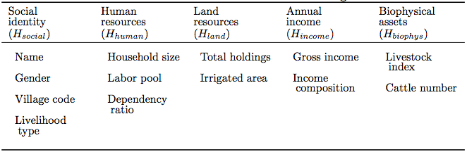
Table 1. List of attributes of household agent - 2.14
- Hprofile comprises social, human, biophysical, land, and financial variables, giving a broad characterization of the household's assets. The particular variables are specific to our case study (Table 1). The changes represented by the update rules FH-internal comprise those variable changes that are not controlled by other model components. Here, these refer to variables related to the small-scale demography of animate beings, including the livestock index Hlivestock, the cattle number Hcattle, the household size Hsize, the laborer to household size ratio Hlaborer, and the age of the household head Hage. Le (2005) argues that since these types of variables are difficult to predict, they should best be modelled as being subjected to only stochastic variations, as illustrated by Hlivestock:

(2) where rand() generates a random floating number between the two assigned numbers, and σlivestock is the standard deviation of the livestock index variable Hlivestock. Finally, the variable Hlabor-pool is dependent on the labor composition of the household, which we thus modelled via linear regression of household size and dependency ratio.
- 2.15
- For modelling age, and thus also death and creation of household heads, we use the model by Le (2005) (equation 3).

(3) where Hage is an agent's age, Agemax, Agemin, and Agestd are maximum, mean, and standard deviation of the original empirical age dataset, respectively, and rand() is a function that draws a random floating number between zero and the assigned number. Note that Le (2005) justifies the use of the aging model by saying that he "approximates" the age of new household heads by assigning them random values around the mean. Thereat, he does not indicate whether the model was informed by theory or is specific to his case study, which suggests that he intends to present a general model for household agent update as part of his framework.
- 2.16
- The third component of household agents, the LandscapeVision did not find application here, since we restricted the model to cultivation of own patches; we found that land rent, if any, locally follows informal channels and is difficult to replicate with the concept of simple search radii. Due to lack of network data, we therefore omitted this option for this version.
- 2.17
- Finally, the LUDAS framework envisages the behavioral parameters (Hbehavior) of the household to be dependent on its livelihood class. The livelihood classes are characterized by the set of agents in the class, the class id (Lid) and the behavioral parameters of that class (Lbehavior). Typical livelihood classes have been identified by applying Principle Component Analysis and k-mean Cluster Analysis in this order to a range of explanatory assets using the sustainable livelihood framework (for details Le 2005; Schindler 2010). The LUDAS framework follows the thought that a household's livelihood influences its survival strategy by assigning labor budgets to survival strategies and preferences to land uses according to the livelihood class of a household.
- 2.18
- Survival strategies prevalent in the study area comprise non-farm activities, livestock raising, and cultivation. Following this mindset, the behavioral parameters that we identify with a livelihood class include parameters for rainfed land-use decision making, in particular preference coefficients for land-use type i Hpref-ik, k = 1, …, 6, and labor days to be spent on land-use type i Hlabor-i. Dry-season cultivation choices were not elaborated in more detail in the model, since local irrigation seems to have already reached its limit and has only a low spatial extent (Schindler 2010). In addition, labor budgets are assigned to survival strategies other than rainfed land use. Annual gross non-farm income Hnon-farm-income and gross income from dry-season cultivation Hdry-cult-income are calculated in accordance to these assigned labor budgets. Gross income from livestock Hlivestock-income was approximated by other factors, such as the livestock available.
- 2.19
- To allow agents to adapt their livelihood strategy, an AgentCategorizer allows the switch of livelihood class in each time step through a distance model using the same explanatory variables as those used for livelihood classification. This way, if an agent has undergone significant changes in livelihood assets, he will possibly adopt another livelihood class and thus strategy. The distance model assigns each agent the class with smallest Euclidian distance between group mean and the agent's values in explanatory variables.
Household decision-making mechanism
- 2.20
- DECISION is the household decision-making module embedded in the household agent, determining land-use type and management of owned patches. Only owned patches are cultivated as far as household labor allows.
- 2.21
- For assigning land-use types to owned patches, first the utility of each land-use type for a random owned patch is calculated. The LUDAS framework envisages the calculation of utility of the patch for a specified land-use type through multinomial logistic regression of survey data. The selection among land-use types is implemented using the original ordered choice used by at least Le (2005) and Kaplan (2011). That is, the utilities are ranked, and one land-use type tested after the other. Thereby, the utilities, which are between 0 and 1, are used as probabilities. In particular, the first land-use type is tested, i.e. chosen in case a random number is smaller than the probability (= utility), then the second, etc. until a land-use type is chosen. Le (2005) justifies the use of ordered choice by comparing the main three models for discrete choice (Benenson and Torrens 2004), and their strength to represent bounded rationality (Simon 1982). Thereby, he argues that "the order in which options are taken for consideration may be important" in human choice, and that "given an option preliminarily picked, the final decision to choose this option is still the result of testing and rejecting with the choice probability". Note that he does not make a reference to case-study specifics here.
- 2.22
- The set of explanatory variables for these utilities is comprised of one explanatory household variable and one environmental variable per land-use type (for details see Table 3 later in this text). In all of the reviewed LUDAS publications the range of explanatory variables for land-use choice is justified through ethnographic methods. In particular, each variable is presented with a hypothesis for how it affects land-use choice based on qualitative understanding from field work, followed by a statistical evaluation of the hypothesis. However, this evaluation was not used to exclude variables from the model. The (non-stated) reason is probably that a non-significant statistical correlation can rarely be easily regarded as a valid criterion for exclusion. That is, the non-significance does not necessarily need to be due to a lack of explanatory power but can be due to other reasons such as e.g. a weak data set.
- 2.23
- The hypotheses for the basic set of variables used here (see Table 3) are i) that the majority of cereals are grown in direct proximity to the homestead because they depend on household manure (distance to house), ii) that rice is grown in areas with low elevation where rainwater can cumulate in sufficient quantities (elevation), iii) that groundnuts are usually grown on more gravelly and sandy soils (soil depth), which were claimed to be much less suitable for the other local staples, and iv) that the land area per person in the household mainly influences whether the land-use pattern is more oriented towards subsistence farming consisting of cereals or rather towards cash cropping covering groundnut and rice (area per capita). Multinomial logistic regressions verify hypotheses i), ii), iii).
Landscape agent
- 2.24
- The landscape agent or patch is characterized by a set of attributes (Pactual) (Table 2), and a set of internal ecological sub-models that perform patch dynamics (FP-internal):

(4) 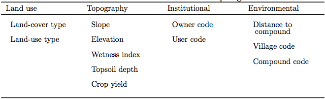
Table 2. List of attributes of landscape agent To keep the model as simple as possible, we restricted the ecological sub-models to crop production and subsequent income generation.
Crop production
- 2.25
- Conceptually, crop yield can be described as a function of climate, soil/water and management (Le 2005). Following this mindset, we developed crop production functions using simple linear regression applied to main local soil-water and management factors (equation 5), which are subjected to stochastic variations induced by climate and other external factors (equation 6). Labor has been cited as the most important production factor in rural Africa (Wiebe et al. 1998), while the wetness index (for equation see Le 2005) represents the soil moisture due to runoff, being the major water source in the rainy season. In the absence of more appropriate soil data, soil depth was used as a proxy for soil fertility.
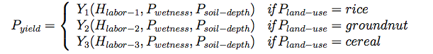
(5) where Yi are linear functions. Pyield is the yield in monetary terms using price data from 2006 (Schindler 2010), which is further subjected to climatic and other external factors:

(6) where Gvar is randomly drawn in each time step from the normal distribution N(1,σ), where we set σ to 0.19. The latter value represents the degree of variability of yields in Ghana and is based on national production data of cereals from 1967–2008 (World Bank 2011). Specifically, the value is the standard deviation of the deviations (in percentage) from the trend (calculated by linear regression) to the actual data.
Income generation
- 2.26
- The total annual gross income is the sum of gross income from cultivation and non-cultivation activities (equation 7).

(7) where Hrainy-cult-income is the sum of the yield in monetary terms of all cropped patches by the household. Hlivestock-income is simply described by a live-weight gain, livestock stock, and the local price (equation 8).

(8) where we used a live-weight gain of 8.75 % (compare van Keulen and Breman 1990) and set GTLU-price to the average annual local market price for a cattle in 2006.
GH-LUDAS: Alternative designs
- 2.27
- Here, we present the alternatives and their associated justifications. To enable more convenient comparison to the original design, we adhere to the structure of the previous section.
Household agent
- 2.28
- For this part of the model we suggest an alternative way of modelling household agent aging. In particular, we suggest using the model by Freeman (2005), Stolniuk (2008) and Arsenault (2007) (equation 9). Equally to the model by Le (2005) (equation 3), it was presented in a form that suggested universality. In particular, it envisages letting agents die with age-specific probabilities, and be replaced by agents one generation younger. Following the implicit implication by Le (2005) that his model is informed by general laws, we can equally use another type of model that makes the same case.

(9) where Dage is the death probability for the agent's age class, and Gint the generation-cycle interval. Here, the generation-cycle interval was set to 27 years after Lamptey et al. (1978), and the age-specific death probabilities were extrapolated using data from Khagayi et al. (2011).
Household decision-making mechanism
- 2.29
- For household decision making we propose two modifications. These comprise the mode of choice among land-use utilities and the utilities' set of explanatory variables.
- 2.30
- For justifiying ordered choice for the mode of choice, Le (2005) cites the most common theoretical utility-based models presented by Benenson and Torrens (2004), including ordered choice, random choice, and satisfier choice. For selection among them, Le (2005) uses the argument that humans may have a preference bias towards better options, as implemented by ordered choice. But just as one can find theoretical arguments that support this model, we apprehend that one can find theoretical arguments for also choosing a different model. We suspect that this choice remains a matter of vote by the modeller as long as it is not informed by case-study specifics. For illustration, we implement random choice, using the (to us more perspicuous) argument that simulated land-use composition becomes distorted when using ordered choice. In particular, using ordered choice, choice probabilities become biased by the rank of a land-use type, i.e. land-use types with higher rank are disproportionally more often selected. This clearly leads to a different land-use composition than the observed one. Random choice, on the other hand, simply envisages to select the land-use types according to their observed/calculated probability. The point is that in case a choice bias indeed exists among land users, it is already reflected in the observed land-use probabilities that are used for regression. Therefore, we believe the probabilities that are calculated by regression should be left as they are.
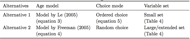
Table 3. Model design alternatives 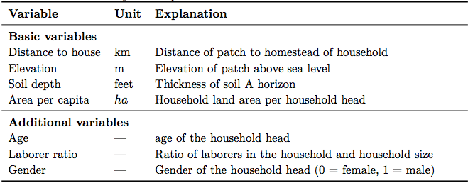
Table 4. Explanatory variables used for land-use choice model 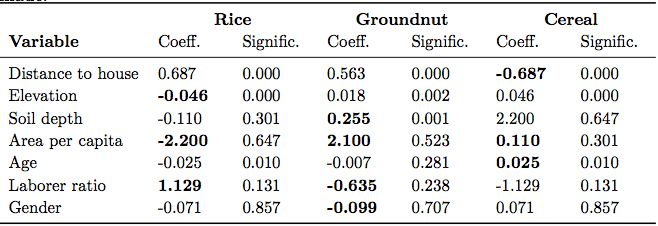
Table 5. Correlation coefficients and significance of the selected variables in the m-logit model for explaining land-use choice. Figures in bold refer to hypotheses made. - 2.31
- With regard to the variable set, the LUDAS strategy of justification of explanatory variables consists of candidate selection and their hypothesized effect through ethnographic methods, followed by a statistical evaluation of these hypotheses. To remind, the purpose of the statistical evaluation was not to exclude variables but to give support for existing hypotheses. In addition to this problem of assessing the necessity of variables, we find this validation strategy also weak in assessing their sufficiency. That is, the availability of hypotheses is not a valid criterion for the completeness of the variable set; other important variables may exist that one has simply missed during field-work analysis. We therefore propose an extended set through adding other important household variables whose hypotheses we found weaker and less obvious at the first sight. The hypotheses for these additional variables (Table 4) are v) that older farmers prefer to stick to the more traditional cereal crops of millet and sorghum (age), vi) that female household heads tend to grow more groundnuts as the groundnut is a typical women's crop (gender) (see also Naidu et al. 1999), and vii) that households with more available labor tend to focus on the labor-intensive but more profitable rice crop (laborer ratio). Multinomial logistic regression verified only hypothesis v) (Table 5).
Simulation results
- 3.1
- To test the effects of using design alternatives described in the previous section on simulated land-use change, we conducted simulations. Since we have two alternatives for each of the three described model parts (Table 3), we obtained eight model versions.
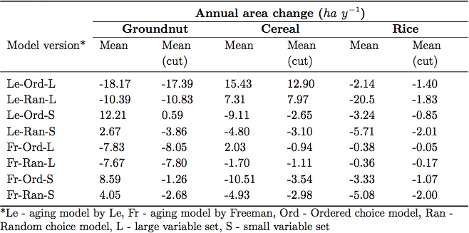
Table 6. Means of simulated annual area change of land-use types over model versions - 3.2
- Each version was simulated 15 times for a period of 30 years, a period for which we believe the model should be able to reproduce the local land-use system. At the first sight, the differences among simulated land-use changes among versions are clearly visible (Figure 2). For example, the use of model version Le-Ord-L resulted in a decrease in groundnut area and an increase in cereal area, while e.g. model version Fr-Ord-S yielded opposite trends (Table 6).
- 3.3
- Also statistically, these differences are significant. A Kruskal-Wallis test for independent samples showed that the medians of mean annual change in groundnut and cereal were significantly different over model versions (using a significance level of 0.05). Here, with mean annual change we refer to the mean of annual changes over the 30-year period, while the median denotes the median of these means over all 15 runs. The non-parametric Kruskal-Wallis test was chosen because the variances of the mean annual change were inhomogeneous, and because the samples were independent.
- 3.4
- However, looking at the trends, e.g. specifically the groundnut trends (Figure 2), one may argue that the value is spiking during the first three years, and that this may be the reason for the statistical significance in difference. These spikes may possibly be caused by the need of the model to first adjust itself. We therefore conducted the Kruskal-Wallis test once more after cutting off the first three values. But still with the cut-off, mean annual change in land-use area showed means with even opposite signs for cereal and groundnut (Table 6). In addition, the medians of mean annual change were here also significantly different over model versions for all land-use types using the Kruskal-Wallis test.
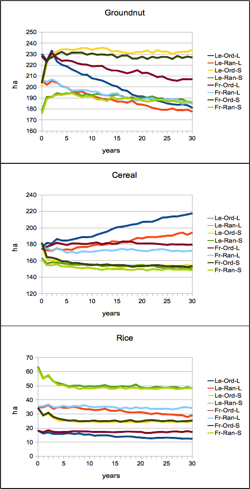
Figure 2. Simulated area of land-use types over model versions 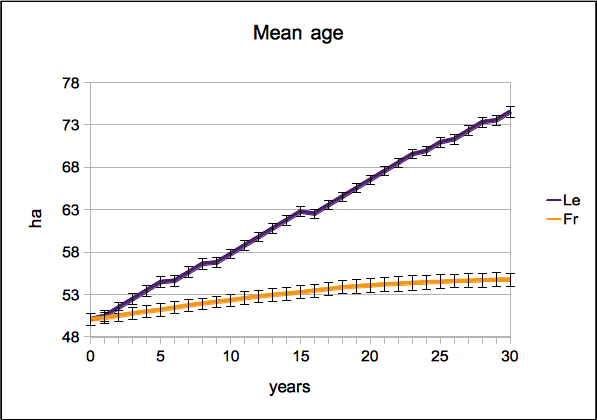
Figure 3. Simulated mean age and standard deviation using the aging model by Le (Le) and Freeman (Fr), repeating each model run 15 times. 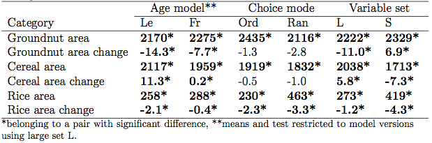
Table 7. Means of annual area (ha) and area change (ha/year) of land-use types over the simulation period. The data set for calculating means was either divided by age model used, by choice mode used, or by variable set used (Fr = aging model by Freeman (2005), Le = aging model by Le (2005), Ran = Random choice, Ord = Ordered choice, S = small variable set, L = large variable set). - 3.5
- The effects of alternatives in the versions also seem to follow clear patterns. Looking more closely at the trends (Figure 2), it seems that the use of the age model by Le (2005) led to higher levels of cereal area compared to the corresponding versions using Freeman (2005), and to lower levels in rice and groundnut. This impression was validated by a Kruskal-Wallis test of the mean annual land-use areas between versions using different age models (Table 7). Here and below, the non-parametric Kruskal-Wallis test was applied in all cases because the conditions for parametric tests were violated in most cases, and because the values were independent. In cases where conditions were not violated, a one-way ANOVA was applied, leading to the same result in these cases. For both types of tests, a significance level of 0.05 was used.
- 3.6
- The reason for the significant difference between versions using different age models is that the use of the model by Le leads to a higher increase in age in the long term than the model by Freeman (Figure 3), and that older farmers have a preference for the more traditional cereal crops while the younger farmers prefer the more cash-oriented rice and groundnut crops. That the model by Le (2005) leads to such a larger increase in age is due to the design of the model: when agents reach the maximum age they are assigned an average age. This way, the presence of old ages is maintained, while the presence of correspondingly young ages is diminished. This leads to a long-term shift of average age in the positive direction over time until it converges (for a detailed analysis see also Schindler 2012). Since the mean age grows over time, we also have correspondent significant differences in annual land-use area change among both version types, using the Kruskal-Wallis test (Table 7).
- 3.7
- The differences between using the large or small variable set follow the same pattern, due to the same reasons. Since age was part of the large set in the land-use choice model, but not of the small set (Table 4), versions using the large set had significantly higher levels of cereal and lower level of groundnut and rice areas, compared to the version using the small set. Also, the cereal and groundnut area changes are in line with this argument in a significant fashion.
- 3.8
- Finally, the use of ordered choice led to a significantly higher level of groundnut and cereal areas than compared to random choice, and to a lower area level for rice. The reason is that groundnut and cereal usually have land-use choice probabilities near 50 % while rice probabilities are very low, and that in ordered choice high probabilities are increased while lower probabilities are even decreased (see section 2.1.2).
Discussion
- 4.1
- The results indicate that the design strategy of the LUDAS model family may not be appropriate in this form. The primary problem is that Le (2005) did not explicitly state which part of his model pertains to a generalizable framework, and which part is case-specific. Together with a lack of theory on land-use change, this lack of explicitness embodies the danger of adopting the framework or parts of it and to mistake it as theory or a valid platform to borrow tools from. We dare to conclude that the generalizability of the framework or parts of it must be (re)defined for further scrutiny for this purpose.
- 4.2
- Yang and Gilbert (2008) report on a model-development experience during which they employed similar ethnographic elicitation methods as we did. Their observation is similar to ours in that they report of the need to include unjustifiable constants and that "the model had to be made more definite than the ethnographic record could justify" (Yang and Gilbert 2008). But they add that this may not pose difficulties provided that the model represents at some abstract level the qualitative understanding of mechanisms. In our case, the choice of design strategy did not leave room for qualitative design of the model framework. The causes for the inconsistencies among model versions are at least partially due to the type of theoretical framework used; for instance, the framework envisaged the employment of utilities and the selection of a choice mode. But the restriction to the utility model rendered a qualitative validation of the choice mode impossible, since these concepts did not seem to reflect the way land-use decisions are made in the study area. Rather, we believe that locals apply a heuristic approach, where single factors are decisive and cannot be outweighed by other factors - as assumed in the utility concept employed here. More formally, Brandstätter et al. (2006) have for instance shown that a heuristic approach was better able to predict the majority choice of participants in gambles than the expected utility approach. For our case study, a more appropriate alternative to the utility modelling approach may therefore have been a participatory approach leading to a heuristic model, such as e.g. Ethnographic Decision-Tree Modelling (Gladwin 1989). But the use of such an approach would have violated the design strategy selected. The question is therefore what alternative design strategies do exist for modelling land-use change empirically?
- 4.3
- Here is where the study of methodology in social science could be worthwhile. Geller and Moss (2008) provide a demonstration of how to construct a model driven by case-study evidence employing knowledge-eliciting techniques and theory from social science. Especially evidence-driven (e.g. Alam et al. 2007) or participatory modelling approaches such as companion modelling (Barreteau et al. 2003; E_tienne 2011) have been frequently applied to validate model design. Companion modelling envisages models to be developed interactively with stakeholders, thereby tapping valuable local knowledge and accounting for the difference in perspectives on system functioning (Barreteau et al. 2003). Other qualitative but less expensive methods for model development have been proposed by Polhill et al. (2010). But scholars note that even if qualitative knowledge is used to specify agents, this knowledge should be converted into utility functions only with caution. In particular, they argue that results can be sensitive to parameterizeration and the model form used (Edmonds 2006; Moss 2008).
- 4.4
- We would like to note, however, that for the purpose of land-use modelling, such participatory methods may not be suitable for all model components. Especially where slow and covert processes at higher scales are at place, such as in land-use change, these processes may not be part of the perception of stakeholders. We therefore believe that land-use modelling should draw on theory where evidence is weak, and draw on evidence where theory is weak, and clearly state assumptions as such when not supported by either of them. Regarding the latter, we consider the type of aging model used in this study as an example where assumptions should have been clearly stated as such. In Schindler (2012) we conducted an in-depth comparison of different designs of such aging models. There, we showed that they lead to significantly different age patterns over time, and propose an aging model whose assumptions are clearly externalized.
- 4.5
- Another currently emerging way to systematically develop land-use change models consists of theoretical research guides to systematically unfold a human-environment system's processes at several scales, such as the one offered by Scholz (2011). A second strategy consists of the development of land-use change theory that can inform model development. Here, we share the argument by Moss and Edmonds (2005) that simulation can be used to inform theory development. However, like them, we believe that theory validity can only be achieved when the design of the agents does not draw on any prior unvalidated theory. Thus we believe that more stringent model documentation and the choice of more appropriate methodology in model design validation can greatly contribute to this purpose, but also to better assess a model's validity by other scholars.
References
-
ADU S. V. (1969). Soils of the Navrongo-Bawku Area, Upper East Region, Ghana. Soil Research Institute, Kumasi, Ghana.
ALAM S. J., Meyer R., Ziervogel G. and S. Moss. (2007). The Impact of HIV/AIDS in the Context of Socioeconomic Stressors: an Evidence-Driven Approach. Journal of Artificial Societies and Social Simulation 10(4): 7. https://www.jasss.org/10/4/7.html
ARSENAULT A. M. (2007). A Multi-Agent Simulation Approach to Farmland Auction Markets: Repeated Games with Agents that Learn. Master thesis. University of Saskatchewan.
ASHLEY C. and D. Carney. (1999). Sustainable livelihoods: Lessons from early experience. London: Department for International Development (DfID).
BARRETEAU O. and others. (2003). Our companion modelling approach. Journal of Artificial Societies and Social Simulation 6(1), 1. https://www.jasss.org/6/2/1.html
BENENSON I. and P. M. Torrens. (2004). Geosimulation: Automata-Based Modeling of Urban Phenomena. London: John Wiley & Sons. [doi:10.1002/0470020997]
BRANDSTÄTTER E., Gigerenzer G. and R. Hertwig. (2006). The priority heuristic: Making choices without tradeoffs. Psychological Review, 113, 409-432. [doi:10.1037/0033-295X.113.2.409]
EDMONDS B. (2006). Assessing the safety of (numerical) representation in social simulation. In Billari F, Fent T, Prskawetz A and Schefflarn J (eds.) Agent-based computational modelling, Heidelberg: Physica Verlag, pp. 195-214. [doi:10.1007/3-7908-1721-X_10]
ELLIS F. (2000). Rural Livelihoods and Diversity in Developing Countries. Oxford: Oxford University Press.
ÉTIENNE, M. (ed.). (2011). Companion modelling. A participatory approach to support sustainable development. Versailles: Éditions Quæ.
FREEMAN T. R. (2005). From the ground up: An agent-based model of regional structural change. Master thesis. University of Saskatchewan.
GELLER A. and S. Moss. (2008). Growing QAWM: An evidence-driven declarative model of Afghan power structures. Advances in Complex Systems 11(2): 321-335. [doi:10.1142/S0219525908001659]
GLADWIN C.H. (1989). Ethnographic decision tree modeling, Qualitative Research Methods Series 19, Sage Publications, Newbury Park, 96 pp.
KAPLAN M. (2011). Agent-based modeling of land-use changes and vulnerability assessment in a coupled socio-ecological system in the coastal zone of Sri Lanka. Dissertation. University of Bonn. Ecology and Development Series 77. Göttingen: Cuvillier Verlag.
KHAGAYI S., C. Debpuur, G. Wak, and C. Odimegwu. (2011). Socioeconomic status and elderly adult mortality in rural Ghana: Evidence from the Navrongo DSS. African Population Studies Journal 2011.
LAMPTEY P., D. N. Nicholas, S. Ofosu-Amaah, and I. M. Lourie. (1978). An Evaluation of Male Contraceptive Acceptance in Rural Ghana. Studies in Family Planning 9(8): 222-226. [doi:10.2307/1965867]
LE Q. B. (2005). Multi-agent system for simulation of land-use and land-cover change: A theoretical framework and its first implementation for an upland watershed in the Central Coast of Vietnam. Ecology and Development Series 29. Göttingen: Cuvillier Verlag.
LE Q. B., S. J. Park, P. L. G. Vlek, A. B. Cremers. (2008). Land use dynamic simulator (LUDAS): A multi-agent system model for simulating spatio-temporal dynamics of coupled human-landscape system. 1. Structure and theoretical specification. Ecological Informatics 3(3): 135-153. [doi:10.1016/j.ecoinf.2008.04.003]
LE, Q. B. (2006). Digital Elevation Model (DEM) at 15 and 30m resolutions for Anayare and Atankwidi catchments downscaled from USGS SRTM Elevation data (at the resolution of 92.53 m). GLOWA-Volta Project Geo-database.
MARTIN N. (2005). Development of a water balance for the Atankwidi catchment, West Africa - A case study of groundwater recharge in a semi-arid climate. Dissertation, Georg-August-Universität, Göttingen.
MIYASAKA T., Q. B. Le, T. Okuro, X. Zhao, R. W. Scholz, K. Takeuchi. 2012. An agent-based model for assessing effects of a Chinese PES programme on land-use change along with livelihood dynamics, and land degradation and restoration. In: R. Seppelt, A.A. Voinov, S. Lange, D. Bankamp (Eds.). International Environmental Modelling and Software Society (iEMSs) 2012 - International Congress on Environmental Modelling and Software Managing Resources of a Limited Planet, Sixth Biennial Meeting, Leipzig, Germany, 01-05 July 2012.
MOSS S. (2008). Alternative Approaches to the Empirical Validation of Agent-Based Models. Journal of Artificial Societies and Social Simulation 11(1), 5. https://www.jasss.org/11/1/5.html
MOSS S. and B. Edmonds. (2005). Towards Good Social Science. Journal of Artificial Societies and Social Simulation 8(4),13. https://www.jasss.org/8/4/13.html
NAIDU R. A., F. M. Kimmins, C. M. Deom, P. Subrahmanyam, A. J. Chiyembekeza, and P. J. A. van der Merwe. (1999). Groundnut Rossette: A Virus Disease Affecting Groundnut Production in Sub-Saharan Africa. Plant Disease 83(8): 700-709. [doi:10.1094/PDIS.1999.83.8.700]
NUNIFU T. K. and H. G. Murchison. (1999). Provisional yield models of Teak (Tectona grandis Linn F.) plantations in northern Ghana. Forest Ecology and Management 120, 171-178. [doi:10.1016/S0378-1127(98)00529-5]
PARKER D. C., S. M. Manson, M. A. Janssen, M. J. Hoffmann, and P. Deadman. (2003). Multi- agent system models for the simulation of land-use and land-cover change: a review. Ann. Assoc. Am. Geogr. 93(2): 314-37. [doi:10.1111/1467-8306.9302004]
PARKER D. C. , T. Berger, and S. M. Manson (eds.). (2001). Agent-Based Models of Land-Use and Land-Cover Change. Proceedings of an International Workshop October 4-7 2001, Irvine, California, USA.
POLHILL J. G, Sutherland L.-A. and N. M. Gotts. (2010). Using Qualitative Evidence to Enhance an Agent-Based Modelling System for Studying Land Use Change. Journal of Artificial Societies and Social Simulation 13(2): 10. https://www.jasss.org/13/2/10.html
SCHINDLER J. (2010). A multi-agent system for simulating land-use and land-cover change in the Atankwidi catchment of Upper East Ghana. Dissertation. University of Bonn. Ecology and Development Series 68. Göttingen: Cuvillier Verlag.
SCHINDLER J. (2012). The importance of being accurate in agent-based models - an illustration with agent aging. In: Guttmann C. and I. J. Timm (eds.). Proceedings of the 10th German Conference on Multiagent System Technologies, Trier - Germany, October, 10th-12th 2012, Springer.
SCHOLZ R.W. (2011). Environmental literacy in science and society. From knowledge to decisions. Cambridge University Press, Cambridge, UK. [doi:10.1017/CBO9780511921520.018]
SIMON H. A. (1982). Models of Bounded Rationality, Volume 1, Economic Analysis and Public Policy, Cambridge, Mass., MIT Press.
STOLNIUK P. C. (2008). An Agent-Based Simulation Model of Structural Change in Agriculture. Master thesis. University of Saskatchewan.
VAN Keulen H and H Breman (1990) Agricultural development in the West African Sahelian region: a cure against land hunger? Agriculture, Ecosystems and Environment, 32 (1990) 177-197. [doi:10.1016/0167-8809(90)90159-B]
VILLAMOR G. B. (2012). Flexibility of multi_agent system models for rubber agroforest landscapes and social response to emerging reward mechanisms for ecosystem services in Sumatra, Indonesia. Dissertation. University of Bonn. Ecology and Development Series 88. Göttingen: Cuvillier Verlag.
WIEBE K. D., M. J. Soule, and D. E. Schimmelpfennig. (1998). Agricultural Productivity and Food Security In Sub-Saharan Africa. In: Food Security Assessment GFA-10, Economic Research Service, Washington DC.
WORLD Bank (2011) Country indicators: Cereal yield (kg per hectare) http://data.worldbank.org/indicator/AG.YLD.CREL.KG
YANG L. And N. Gilbert. (2008). Getting away from numbers: Using qualitative observation for agent-based modelling. Advances in Complex Systems 11(2): 1-11. [doi:10.1142/S0219525908001556]