Abstract

Space plays an important role in the transfer of information in most societies that archaeologists study. Social networks that mediate learning and the transmission of cultural information are situated in spatial environments. This paper uses an abstract agent-based model to represent the transmission of the value of a single "stylistic" variable among groups linked together within a social network, the spatial structure of which is varied using a few simple parameters. The properties of the networks are shown to clearly affect both the overall amount of variability that is produced by the cultural transmission process and the spatial organization of that variability. The relationships between network structure, network properties, and assemblage variability in this simple model are patterned and predictable. This suggests that changes in the spatial structure of social networks may have important implications for interpreting patterns of artifact variability in large-scale archaeological assemblages.

Keywords:

Social Networks, Cultural Transmission, Spatial Analysis, Network Structure, Network Properties, Archaeology

Introduction

1.1

All human societies are comprised of individuals connected to one another by overlapping arrays of social ties that together constitute a social network. Social networks are emergent phenomena that both influence and are produced by the behavior of individuals (Barnes 1972; Blau and Scott 1962; Radcliffe-Brown 1940). They channel information, people, genes, and resources and can be used to define the extent of a social system. The importance of social networks to all human societies makes them a fundamental and enduring topic of anthropological, archaeological, and sociological interest.

1.2

Social networks articulate with material culture because learning is situated in social contexts. Closely related, co-resident persons are typically instrumental in the generational (i.e., "vertical") transfer of craft traditions: parents (and related individuals) teach children (Bamforth and Finlay 2008; Berry and Georgas 2009; Minar 2001; Shennan and Steele 1999). The high density of ties within local groups allows for the rapid "horizontal" peer-to-peer transfer of information related to technological innovations and improvements (seeBerry and Georgas 2009; Bettinger and Eerkens 1999:237; also Schiffer and Skibo 1987:597). In neither case is information transfer random: interactions among individuals are mediated by social ties. Transfer of both kinds of information is subject to human error, which is a source of variability in material culture. Space plays an important role in social learning in most societies that archaeologists study because of the importance of face-to-face interaction for the transfer of information. Thus we can view archaeological artifacts as the material residues of spatially-situated, network-mediated systems of social learning and information exchange.

1.3

Archaeologically-visible changes in the patterns of variability in material culture are often attributed to changes in the scale or structure of social networks (e.g., see Banks et al. 2009; Conkey 1980; Gamble 1986; Isaac 1972; Koldehoff and Loebel 2009; White 2006;Wobst 1976, 1977). Relationships between network structure and patterns of variability in material culture are not well-understood, however, as it is impossible to directly observe how large-scale temporal and spatial patterns emerge from the "rules" of cultural transmission and social network formation that guide behavior at the level of the individual or group. Both ethnographic studies (e.g.,White and Johansen 2005; Yellen and Harpending 1972) and studies of abstract model networked systems with a spatial component (e.g.,Axelrod 1997; Klemm et al. 2003) suggest that these relationships are likely to be neither simple nor intuitively obvious. Making sound inferences about the structure of prehistoric social networks or the presence of social boundaries based on material remains will require building a theoretical basis for understanding the relationships between these phenomena (seeWhite 2012).

1.4

Current approaches to studying cultural transmission and its material correlates generally fall at either end of a "micro" to "macro" continuum of temporal and spatial scales of analysis/interpretation (Stark et al. 2008). Cultural transmission among living populations is, necessarily, studied at the small scales of time and space that are possible using ethnographic methods of direct observation (e.g., see Minar and Crown 2001; Stark et al. 2008). Archaeological studies, conversely, are dominated by the use of equation-based models to interpret long-term changes in artifact variability (e.g., Bentley and Shennan 2003; Eerkens and Lipo 2005; Hamilton and Buchanan 2009; Neiman 1995; but see also Premo and Scholnick 2011). These models often make assumptions that individuals interact randomly (i.e., "panmixia") or that individuals can more-or-less accurately copy the mean of a large population.

1.5

The gap between these two scales of analysis is an important one: the macro-scale (archaeologically visible) outcomes of micro-scale cultural transmission behaviors are potentially affected by the structured (i.e., non-random), network-mediated, spatially-situated interactions that are typical of human systems. Numerous studies have shown that differences in network structure affect the behavior of both model and real-world systems mediated by these networks (e.g., see Klemm et al. 2003; Newman 2000; Watts 2004; Watts and Strogatz 1998). Relatively small alterations to network structure can have a large effect on how information is transferred across the network: it is often the structure of the connectivity that determines behavior rather than the details of the particular system. This suggests that the structure of interaction may have important, observable effects on the patterns of artifact variability produced by cultural transmission processes mediated by networks.

1.6

Agent-based modeling offers a way to bridge the gap between the micro- and macro-scales of analysis and analyze how micro-scale behaviors "map up" to macro-scale outcomes in environments where interaction is structured rather than random. This paper uses a simple, "abstract" agent-based model (ABM) to consider how the spatial structure of interaction affects the outcomes of a basic cultural transmission process. The model allows parameters affecting the creation of a social network linking a population of groups to be adjusted so that cause-and-effect relationships between network structure, network properties, and patterns of artifact variability can be systematically investigated. Analysis of results from the model shows that network structure has patterned effects on both the amount and spatial organization of variability that is produced by a cultural transmission process. The model is also used to explore the "costs" and "benefits" of differently structured networks. Experimentation with abstract models such as this one constitutes a first step in building the theory required for interpreting patterns of archaeological artifact variability in terms of the social networks that were in operation when those patterns were produced.

TechNet_04: A simple model of cultural transmission in a spatially-situated network

2.1

The TechNet_04 model is one of a series of abstract models that was developed to begin examining the basic relationships between the structure of prehistoric social networks and patterns of variability in material culture. It was constructed to be a simple, flexible platform for running an array of experiments to investigate relationships between network structure, network properties, artifact variability, and the spatial organization of artifact variability.

2.2

The TechNet_04 model was built using RepastJ. The code for the model is available online at http://www.openabm.org/model/3257/version/1/view. Table 1 supplies a description of the main parameters and variables of the model.

Table 1: Main parameters and variables of the TechNet_04 model.
Level	Parameter/Variable	Description
Group	id	Unique identifier for each group
	X, Y	Group's XY coordinates; used by the model to identify locations within the grid
	A, B	Group's AB coordinates; used to calculate geographic distances between cells
	networkList	List of all groups to which a particular group is linked
	variableA	Group's current value of the cultural trait to be transferred
Link	fromGroup, toGroup	Groups connected by the link
	linkDistance	Geographic distance spanned by the link
System	meanNetworkSize	Mean size of all group-level networks in the system
	numLinks	Total number of links in the system-level network
	linkDistMean	Mean geographic distance spanned by links in the system
	longestLink	Longest geographic distance spanned by a link
	meanPathLength (MPL)	Mean path length of system-level network
	clusteringCoefficient (CC)	Clustering coefficient of the system-level network
	meanSD	Mean standard deviation of variableA, averaged over 500 time steps
Model	p	Parameter setting probability of replacement of local links with random links (in rewireMode 1) or addition of non-local links (in rewireMode 2)
	rewireMode	Parameter determining process for rewiring the local-only network that is established at the start of a model run
	rewireRadius	Radius (in tiers of hexagonal cells) within which links to non-local groups can be added when rewireMode = 2
	copyMode	Parameter controlling the population a group will copy: 1 = group copies mean variableA of groups on its networkList; 2 = group copies mean variableA of entire population; 3 = group copies its own variableA; 4 = group copies median variableA of entire population; 5 = group copies deterministic mean that changes according to formula
	pConform	Parameter setting probability that a group will copy some other population of groups (determined by copyMode)
	copyError	Percentage +/- error applied when copying

Spatial environment and population

2.3

The "world" of the model is a two-dimensional, bounded, hexagonal grid. Each cell is the location of a single "group". A hexagonal grid was chosen over a square grid because it reflects how space is used in idealized models of "packed" hunter-gatherer systems (Wobst 1974, 1976) and equalizes the spatial distances of the neighbors of any particular cell at a given number of tiers. A bounded grid was used instead of a torus because the model is intended to represent a social world that has spatial limits.

2.4

A population of groups is created and placed in the world during the set-up phase of the model. Because each cell contains a single group, the number of cells and the population of the world are identical: a 40 x 40 world contains 1600 groups. Each of these groups has an "address" consisting of X and Y coordinates that specify its location in the grid. Each group also has a set of A and B hexagonal grid coordinates that are used to determine spatial distances between groups in terms of the number of cells (Figures 1.A and 1.B).

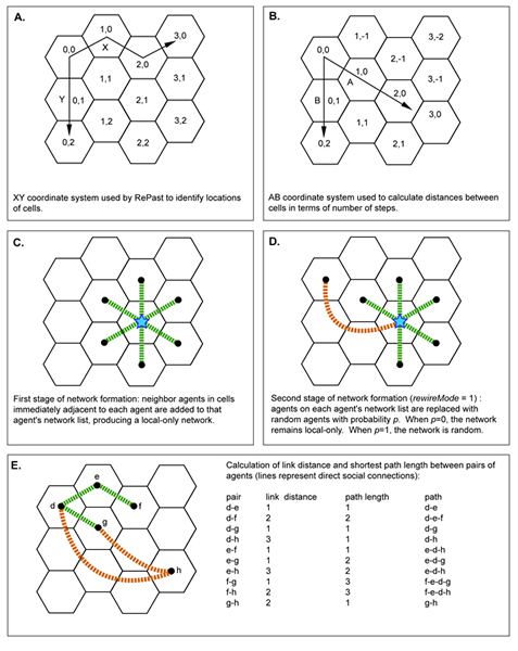
Figure 1. Conceptual illustration of coordinate systems, stages of network formation, and calculation of link distance and path length in the model.

Network structure and properties

2.5

This model is built around the concept that each group can interact with a unique, finite array of other groups to which it is linked. This array constitutes a group's individual network. When two groups are linked, information can be transferred between them. The overlapping networks of individual groups comprise a system-level network that connects all groups within the system.

2.6

Networks are formed at the beginning of a model run and do not change during a model run. Networks are formed through a two-stage process. In the initial stage, each group adds the groups in the immediately adjacent tier of hexagonal cells to its networkList (Figure 1.C). This produces a "local only" network where each group is linked to only those groups who are immediately adjacent to it in space.

2.7

A second stage of network formation "rewires" this local-only network in one of two ways, controlled by the parameter rewireMode. If the value of rewireMode is 1, a group's local links to its neighbors can be replaced by links to random groups (Figure 1.D). The probability of each local link being replaced by a random connection is controlled by the variable p, which is a parameter that can be varied continuously between 0 and 1. Each group goes through its networkList and puts each member of its network in jeopardy of being replaced by generating a uniformly distributed random number between 0 and 1 and comparing it to the value of p set in the model. If the generated number is lower than p, the link with that group is dissolved and a new link is formed with a randomly selected group. Thus when p = 0 (no chance of replacement) the network remains local-only, while a p of 1 (certainty of replacement) produces a network where each link is randomly determined. If a group tries to create a link to a group with which it is already linked, that chance to add a link is lost (i.e., a "duplicate" link cannot be created). Because each link between two groups is two-way, each connection can be in jeopardy of being replaced twice. The link between "Group A" and "Group B", for example, is in jeopardy of being replaced once when "Group A" goes through the rewiring method and (assuming the link was not replaced) once when "Group B" goes through the rewiring method. This procedure of network "rewiring" to interpolate between a regular and a random network is similar to that employed in studies exploring the small-world property (e.g., Klemm et al. 2003; Watts and Strogatz 1998). The main difference is that, in those papers, each link between vertices was only subject to potential rewiring once.

2.8

The bounded nature of the grid and the spatial component of network formation mean that groups located along the edges of the grid have fewer than six other groups in their networks. In a 40 x 40 grid, the mean size of a group's network ( meanNetworkSize) is 5.8 and there are 4641 direct two-way links between groups. The rewiring of the network controlled by p does not affect the total number of direct links in the network: for each link that is dissolved a new one is created. Thus meanNetworkSize remains constant in rewireMode 1.

2.9

Rewiring in rewireMode 1 does affect the distribution of links among the groups in the network, however. When a local group is replaced with a random group, the local group loses a link while the random group gains one. Because of this, it is possible for individual groups to become disconnected from the rest of the population. This occurred with some frequency. In a group of 3000 runs, for example, one or more groups became disconnected from the remainder of the population about 15 percent of the time. The distribution of the number of disconnected groups was right-tailed, with the majority of cases (about two thirds) having only a single group (i.e., less than 0.06 percent of the total population of 1600) disconnected. The maximum number of disconnected groups in a single run was 6 (i.e., about 0.4 percent of the population). Higher numbers of disconnected groups tended to be produced at higher values of p. Groups that become unlinked during rewiring are removed from the world prior to the start of a model run, resulting in small variations in population size. While it is theoretically possible for larger portions of the network to become unlinked from each other, this did happen in practice during use of the model.

2.10

If the value of rewireMode is 2, each group has the chance to create links with non-local groups that are within a specified distance of the group's location. In this mode, a group preserves links with all of its local neighbors and adds links to other, non-local groups. The probability that a group will create a link with a non-local group is, again, controlled by the parameter p. The number of chances each group has to add non-local links was held constant at 6 (the mean size of a local-only group-level network, rounded up from 5.8). In other words, when p = 1, each group will add links to 6 nonlocal groups. The geographic distance between linked groups is constrained by the parameter rewireRadius, which specifies the maximum separation of two linked groups in terms of the number of hexagonal cells. If the value of rewireRadius is 8, for example, a group will form a link with a randomly selected group that is between 2 and 8 tiers distant (it is already linked to all the groups within 1 tier). Because links are added rather than replaced, the mean network size will vary but will always be greater than 5.8 when p > 0.00. If a group tries to create a link to a group with which it is already linked, that chance to add a link is lost (as in rewireMode 1).

2.11

After the network is formed, the model computes the mean path length ( meanPathLength, or MPL) of the network. MPL describes the average social distance from one group to another group in terms of the shortest number of social "steps" between the groups (Figure 1.E). Mean path length is a standard measure of the overall "closeness" or inter-connectedness of the entire network (Lovejoy and Loch 2003). When a group is directly linked to another group, the length of the path between them is 1. When a single intermediary is required to reach one group from another group, the path length between them is 2. The model computes the sum of the path lengths between each unique pair of groups and then divides the total path length by the number of paths. There are 1,279,200 group-group paths in a grid of 1600 groups. The meanPathLength of a 40 x 40 grid with a local-only network is 21.5.

2.12

The variable linkDistance describes the geographical distance traversed by a link in terms of the number of spatial steps (Figure 1.E). The variable longestLink describes the geographic distance traversed by the longest group-group link that exists in the grid. The value of longestLink in a local-only grid will always be 1. When non-local connections are possible, the distance of the longest possible link will be limited by the size of the world in rewireMode 1 and by the value of rewireRadius in rewireMode 2. The variable linkDistMean is the mean distance of all group-to-group links.

2.13

The model also computes the clustering coefficient ( clusteringCoefficient, or CC), which measures the mean inter-connectedness of local neighborhoods (see Watts and Strogatz 1998). The clustering coefficient of each local neighborhood (i.e., the area occupied by a group and the immediately adjacent groups) is defined as the ratio of the number of links that exist among a group's local neighbors to the number of links that are possible among those neighbors (Figure 2). When a group has six neighbors, a total of 15 links are possible among them. If 11 of those links exist, the clustering coefficient in that neighborhood is 0.73. The clusteringCoefficient of the system-level network is the mean of the clustering coefficient of all neighborhoods. The CC of a 40 x 40 grid with a local-only network is 0.4122.

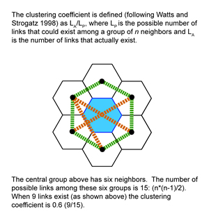
Figure 2. Calculation of clustering coefficient.

Information transfer

2.14

The transmission of cultural information in this model is represented by the transfer of the value of a single real number ( variableA). VariableA is meant to represent some continuously variable, "stylistic" aspect of artifact size, shape, etc., that is subject to copying error and is free to vary through processes such as drift (i.e., change through accumulation of random copying error). Because the purpose of this model is to understand only the relationships between the structure and properties of social networks and the amount and spatial organization of the variability that is produced through simple copying error, no attempt is made to represent sources of variability other than copy error.

2.15

Every group in the world begins a model run with the same value (5) of variableA. This was an arbitrary value selected so the results of some experiments would be directly comparable to those of previous work (e.g., Hamilton and Buchanan 2009). Because variability generated during a run is proportional to the value of variableA, beginning with a different value would affect the results in terms of absolute values but not the overall patterns.

2.16

The transfer of information occurs through copying events. At each step, each group copies the value of variableA either from itself or from some population of groups other than itself (see Table 1). Two parameters control these choices: pConform specifies the probability that a group will copy some "pool" of groups other than itself, while copyMode controls which pool that is. In other words, the variable pConform controls the relative strength of "horizontal" vs. "vertical" transmission, while copyMode determines the population that is copied if a group copies an outside population.

2.17

The variable pConform can be set between 0 and 1. This variable is conceptually the same as the variable lambda (or "strength of bias") used by Hamilton and Buchanan (2009) and "strength of conformance" used by Eerkens and Lipo (2005). When pConform equals 0.30, an agent will copy the value of variableA from a population of groups other than itself with a probability of 0.30. If the group does not copy from an outside population (i.e., does not undertake "horizontal transmission"), it will copy itself by default ("vertical transmission").

2.18

In the event that a group copies the value of variableA from an outside population, the mode of copying ( copyMode) determines the composition of that population: the mean variableA of the groups in its network or the mean (or median) variableA of the entire population in the world. The latter mode of copying does not incorporate any aspects of network-structured interaction (as the group is simply copying some global measure of the central tendency of the population), but allows the model to be used to reproduce the results of equation-based cultural transmission models that do not represent interaction as a structured phenomenon (e.g., Eerkens and Lipo 2005; Hamilton and Buchanan 2009).

2.19

Variability in variableA is generated through copying error (controlled by the parameter copyError) that is applied each time a group copies (whether copying from an outside population or copying itself). The application of error during each copying event is based on the idea that there are inherent constraints in human perception that prevent the detection of slight differences between any two objects, shapes, colors, etc. The amount of error is relative and is typically set at a maximum of +/- 3 to 5 percent based on empirical studies of human perception (e.g., Eerkens 2000; Eerkens and Lipo 2005; Hamilton and Buchanan 2009). This model allows copying error to be either uniformly or normally distributed (Figure 3). When copying error of +/- 5 percent is normally distributed, the mean error is 0 and the 5 percent error is two standard deviations from the mean (errors greater than 5 percent can occur when the error is normally distributed). A uniform distribution of error places a hard limit on the amount of error that can occur. The experiments performed here used a normal distribution of error simply to follow the standard practice in equation-based studies of cultural transmission.

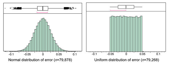
Figure 3. Histograms showing normal and uniform distributions of +/- 5 percent error.

Model operation

2.20

Following creation of the world and the groups, two-stage formation of group-level networks, and setting of parameters controlling information transfer, the model is set into motion. At each time step, each group goes through a sequence of actions during its turn. It first determines whether it will copy variableA from itself or from some outside population (based on pConform). If it copies from an outside population, it determines the population to copy (based on copyMode), calculates the value of variableA to copy, applies copying error, and copies. If it copies itself, it applies copying error to its own value of variableA. The ordering of groups is randomly shuffled each time step. Most of the runs discussed here lasted for 1000 time steps.

2.21

The data output of the model can be adjusted to include different measures and more or less detailed data depending on what is required for analysis. Outputs can range from summary data produced at the end of a run to data about each group at each step.

Experiments and results

3.1

Experiments performed with this model were primarily intended to investigate the relationships between the "rules" of group-level network formation, the resulting structure and properties of system-level networks, and the amount and spatial patterning of variability produced by a simple cultural transmission process. They were also intended to investigate whether spatially-structured interaction produces results that are different from those of equation-based models of cultural transmission that incorporate neither space nor structured interaction. The sections below summarize the experiments and analyses that were used to investigate these aspects of the model. Many of the experimental results presented here were produced to show the relationships among multiple variables. Because these relationships were often nonlinear, some groups of experimental runs were performed to produce additional data pertaining to specific conditions (i.e., runs to produce additional data where p is low).

Implementation of equation-based ACE and BACE models

3.2

Equation-based models are the dominant models of cultural transmission used to interpret archaeological data. These models are typically cast as "accumulated copying error" (ACE) or "biased accumulated copying error" (BACE) models (e.g., Eerkens and Lipo 2005; Hamilton and Buchanan 2009). In the ACE model, transmission is limited to vertical events that represent a generational learning phenomenon, such as between a parent and a child or a master and an apprentice. Individual "lines" of transmission are independent. The overall result of this independence is that the amount of variability among a given set of lines increases through time without constraint. In the BACE model, horizontal or oblique copying events also occur where information is transferred between lines, constraining the amount of variability that is possible.

3.3

The parameters of ACE and BACE models can be implemented within the ABM employed here. The goal of these experiments was not to reproduce all the mathematical nuance of these equation-based models, but to implement them conceptually using a computational platform so that results could be compared to those of the spatially-structured interaction models discussed below. Replicating the results of these equation-based models serves validate the agent-based model utilized here and provide a baseline for further modeling efforts.

3.4

In ACE model, each individual (or "line") is represented by an equation which is run through a series of discrete time steps. The unbiased ACE model can be recreated simply by having each group in the model begin with the same initial value (5) for variableA and copy itself (with +/- 5 percent error, normally distributed) each time step. In this case, each group creates its own ACE "path" which can be plotted vs. time (Figure 4.A). When a large number of runs (n = 1000) is considered, the distribution of outcomes after 100 time steps is lognormal: the median decreases but the mean stays approximately constant (Figures 4.B, 4.C, and 5). Variance increases linearly with time (Figure 4.D). These are the expected outcomes of a drift process based on accumulated, proportional error acting independently within each line (e.g., Eerkens and Lipo 2005:322).

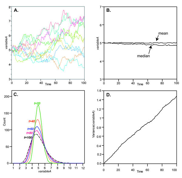
Figure 4. Results from implementation of the ACE model (+/- 5% error, normally distributed): (A) results from 10 individual runs; (B) mean and median of 1000 runs; (C) distributions of variableA at several points in time; (D) variance of 1000 runs. Compare to Hamilton and Buchanan (2009: Figure 1).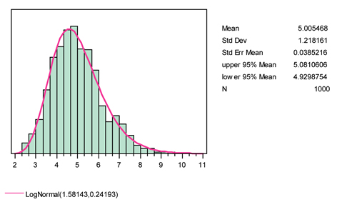

Figure 5. Histogram of variableA at step 100 in the ACE model (1000 runs).

3.5

The BACE model involves the possibility of information transfer between lines. As in the ACE model, an individual in the BACE model is represented by an equation which is run through a series of discrete time steps. The concept of the BACE model can be implemented in the agent-based model by having each group begin with the same initial value (5) for variableA and then copy itself each time step unless it chooses to copy the mean of the population ( n = 100) with probability of 0.30 (0.30 was chosen to mimic the degree of bias used by Hamilton and Buchanan 2009: Figure 2). A sample of ten individual paths within one experiment using copyMode 2 is shown in Figure 6.A. Note that the mean of this batch of individuals does not appear to decrease through time as in the results of Hamilton and Buchanan (2009: Figure 2A). Figures 6.B, 6.C, and 6.D show the mean, median, and variance through time for a series of runs (each point is the average of 20 runs each containing 100 agents). The mean and median stay approximately constant when groups copy the actual population mean ( copyMode = 2). The mean and median both decrease gradually when agents copy the population median ( copyMode = 4). It is only when copying a deterministic equation (decreasing by one half the variance of the copy error every time step, copyMode = 5) that the mean steadily decreases at a rate comparable to that shown by Hamilton and Buchanan (2009: Figure 2). The pattern of change in the variance (Figure 6.D) is similar to that described by Hamilton and Buchanan (2009: Figure 2).

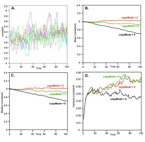
Figure 6. Results from implementation of the BACE model ( pConform = 0.30, +/- 5% error normally distributed): (A) superimposed results of 10 individual groups within one sample run; (B) mean of variableA using three different modes of copying; (C) median of variableA using three different modes of copying; (D) variance of variableA using three different modes of copying ( copyMode 2 = copy population mean; copyMode 4 = copy population median; copyMode 5 = copy formula).

3.6

The standard deviation of variableA ( n = 1600 agents) was calculated at each time step and plotted against time for six runs varying pConform (Figure 7). The relationships between pConform and assemblage variability in these runs is very similar to those depicted by Eerkens and Lipo (2005: Figure 2) and Hamilton and Buchanan (2009: Figure 3). In the BACE model, the "strength of bias" constrains variance and the effect is a nonlinear one.

Figure 7. Effect of varying pConform in the BACE model (one run for each setting, 1600 groups per run). The ACE model conditions are reproduced when pConform = 0.

3.7

In summary, a computational implementation of the ACE and BACE models produced similar patterns of change in variability to equation-based implementations (e.g., Eerkens and Lipo 2005; Hamilton and Buchanan 2009). More copying bias (more horizontal information flow) constrains variability and the effect is nonlinear. A negative drift was present in the median (but not the mean) of the ACE model when the first 100 time steps of 1000 runs were considered. A negative drift in the mean was produced in the BACE model only when the actual population mean was replaced with a deterministic equation (cf. Kempe et al. 2012). The take-away point of these equation-based models is that an increase in copying bias (horizontal transmission) results in a lower overall variability.

Network structure and properties

3.8

A series of experiments was used to investigate how the creation of non-local links affects the structure and properties of the networks in the model. Results from the two different modes of "rewiring" (see above) will be discussed separately.

3.9

When the model is in rewireMode 1, the value of the parameter p is the probability that each link to a local group will be replaced with a link to a random group. When p = 0, all links in the network are between spatially-adjacent groups. When p = 1, all links are randomly determined. Varying p between 0 and 1 interpolates between a regular, local lattice and a random network.

3.10

The changes in network properties that result from changes in p were evaluated by comparing p to the resulting mean path length ( meanPathLength, or MPL) of the network in a series of runs ( n =3000) within a 40 x 40 grid (Figure 8.A). The relationship between p and MPL is clearly nonlinear: replacement of relatively few local connections with random connections results in a reduction in MPL that is disproportionate to the number of links replaced. Random links are "short cuts" that can have a large effect on information flow when they span long distances. The relationships between MPL, p, and the geographic distance spanned by the longest link ( longestLink) are shown in Figures 8.B and 8.C. The likelihood of adding at least one relatively long connection to the grid grows rapidly as p increases from 0. The relatively loose relationship between MPL and longestLink when p is low reflects the influence of the orientation and articulation of each random link when the number of random links is small. The relationship between p and linkDistMean is shown in Figure8.D.

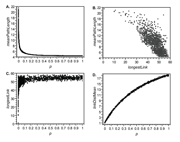
Figure 8. Relationships between variables related to network formation rules, network structure, and network properties ( rewireMode = 1).

3.11

Figure 9 shows MPL and clusteringCoefficient (CC) plotted against p on a logarithmic axis. The values of MPL and CC have been normalized by dividing each data point by the values of MPL and CC when p = 0 (21.5 and 0.4112 respectively). The relationship between p, MPL, and CC compares well to the data presented by Watts and Strogatz (1998: Figure2) in their description of the "small-world" phenomenon. The rapid drop in MPL associated with low values of p produces almost no change in CC: the replacement of a few local links with random links has a significant effect on the global properties of the network but a negligible effect on how the network appears from the local level.

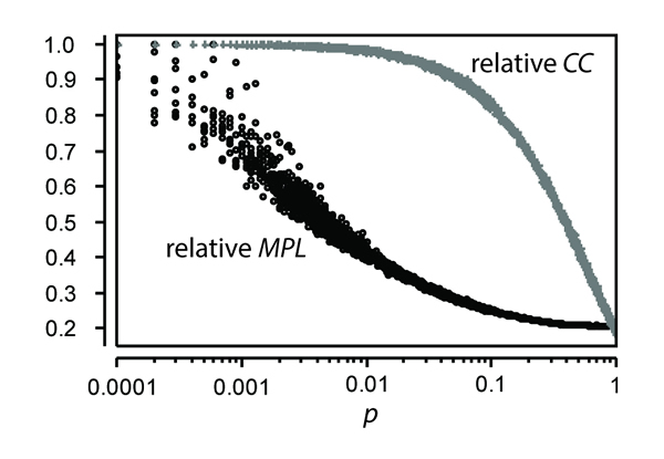
Figure 9. Plot of p versus meanPathLength (MPL) and clusteringCoefficient (CC) with the horizontal axis displayed on a logarithmic scale, rewireMode = 1. Data were normalized by dividing by the values when p = 0 (21.5 for MPL, 0.4122 for CC) in order to plot both variables on the same axis.

3.12

In rewireMode 1, local links are replaced with random links with probability p. These link replacements produce both a "benefit" (a reduction in MPL) and a "cost" (a reduction in CC) in terms of network properties. A simple ratio of "benefit:cost" can be calculated for each run by multiplying the proportional reduction in MPL by the proportional reduction in CC (Figure 10.A). If we assume that longer links are more "costly" to form/maintain, we can alter this calculation to include linkDistMean (Figure 10.B). In either case, it is clear that networks created at values of p between 0.001 and 0.10 offer the best trade-off between benefit and cost.

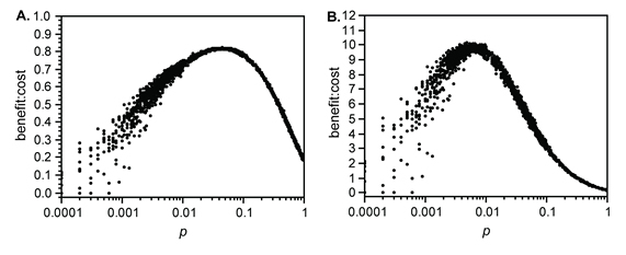
Figure 10. Relationships between p and measures of "benefit:cost" in rewireMode 1. Values in (A) were calculated as: ((21.5- MPL)/17.08) * ( CC /0.4122): 21.5 is the maximum value of MPL, 17.08 is the maximum reduction in MPL, and 0.4122 is the maximum value of CC. Values in (B) were calculated by dividing the values calculated in (A) by ( linkDistMean - 18.24): 18.24 is maximum value of linkDistMean.

3.13

When the model is in rewireMode 2, p is the probability that a group will add a new link to a nonlocal group (see above). The geographic distance of groups to which new links can be added is constrained by the value of rewireRadius, which specifies the number of hexagonal tiers from the group that are included in the search for a new group with which to create a link. Because links are added rather than replaced in this rewiring mode, the value of p has a direct, positive effect on both the total number of links and the mean size of group-level networks.

3.14

A series of experimental runs was used to generate data for several values of p and values of rewireRadius varying from 2 to 57 (i.e., up to the maximum geographic separation of any two groups, the hypotenuse of a 40 x 40). Figure 11 shows the relationship between MPL and rewireRadius for five values of p ( n =500 runs each). The combination of the number of new links added and the geographic distance that those links are permitted to span reduces MPL in a predictable fashion. When p =0.001, between 2 and 18 links (mean of 9.6) were added to the existing local-only network comprised of 4641 two-way links. The addition of these links has a negligible effect on MPL, especially when the value of rewireRadius is low. Higher values of p cause a more rapid drop in MPL even when the rewireRadius is constrained to just 2, 3, or 4 tiers. Increasing the value of the rewireRadius over 10 has little effect on MPL when p > 0.10. The relationships between p and MPL are shown for several values of rewireRadius in Figure 12.

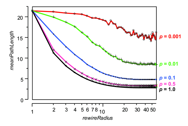
Figure 11. Relationships between rewireRadius and meanPathLength for five values of p in rewireMode 2.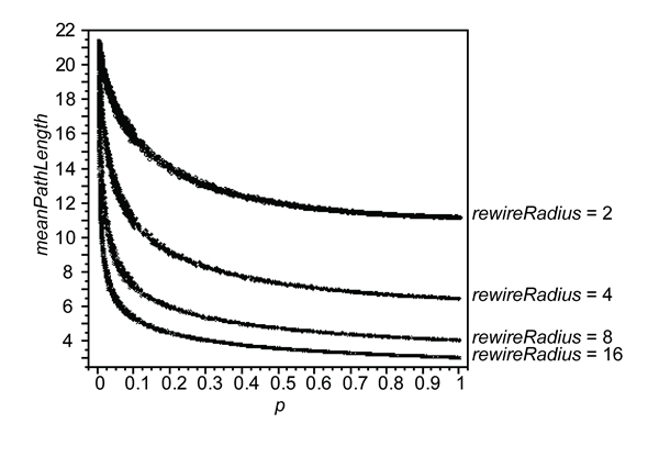

Figure 12. Relationships between p and MPL for several values of rewireRadius, rewireMode 2.

3.15

In rewireMode 2, reductions in MPL are the result of a combination of the number of links added and the geographic distance that those links span. The addition of new links has the potential to increase CC, as groups within local neighborhoods may become more inter-connected as links are added ( CC can only increase or stay the same because existing local links are not removed). Reductions in MPL and increases in CC can both be viewed as "benefits" arising from the alteration of a local-only network structure by the addition of new links. "Costs" associated with adding new links include those associated with forming/maintaining larger group-level networks and those associated with forming/maintaining links spanning greater geographic distances.

3.16

A ratio of benefit to cost can be calculated by incorporating reduction in MPL and increase in CC as "benefits" and increases in meanNetSize and linkDistMean as "costs" (Figure 13). While high values of p (i.e., p =0.5 and p =1.0) are relatively cheap strategies when rewireRadius is 2, they return progressively less benefit per unit of cost as rewireRadius increases past 2. Very low values of p (i.e., p =0.001 and p =0.01) deliver less benefit per unit of cost at low values of rewireRadius but get progressively better as rewireRadius increases. A value of p =0.10 is comparable to high values of p when rewireRadius is 2, but continues to improve until the value of rewireRadius surpasses 5. The low benefit:cost ratios of high values of p stem from the large increases in the sizes of the group-level networks that are created. When the rewireRadius is greater than 2, these large group-level networks add cost without adding much benefit in terms of either a reduction in MPL or an increase in CC. The sparse web of non-local links created at low values of p, conversely, is relatively cheap but produces relatively little benefit until the rewireRadius is large enough to permit the establishment of relatively long links that have a significant impact on MPL. Of the values of p that are investigated, p =0.10 produces the best ratio of benefit:cost when the rewireRadius is less than 8. The density of non-local links is high enough to have a significant impact on MPL but not so high that additional links do not produce a benefit.

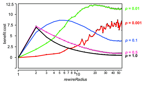
Figure 13. Relationship between measure of "benefit:cost" and rewireRadius for five values of p in rewireMode 2. Values were calculated as (((21.5-MPL)/18.64) * (CC/0.8103))) / ((linkDistMean/15.08) * (meanNetSize/17.78)): 21.5 is the maximum MPL, 18.64 is the maximum reduction in MPL, 0.8103 is the maximum CC, 15.08 is the maximum linkDistMean, and 17.78 is the maximum meanNetSize.

3.17

When the value of rewireRadius is set to the maximum (i.e., 57), the addition of links is a random process controlled by p. Thus many of the relationships between variables seen in rewireMode 1 can be reproduced in rewireMode 2 when new links are created with no spatial constraint.

Amount of variability produced

3.18

As shown above, the structure of a network (how groups are inter-connected) affects its properties (the "ease" of information flow). A lower MPL indicates that, on average, fewer steps are required to get from one group to another group. Information traveling through a network with a lower MPL takes fewer steps to travel to reach all the groups in the network. As MPL decreases, information flow should constrain the variability that is possible (assuming that the propensity for the horizontal transfer of information remains constant), resulting in a positive association between MPL and the standard deviation of variableA. Because standard deviation fluctuates at each time step in any given run, the model was first run for steps 0-499 and then the standard deviation of variableA was calculated during each of steps 500-999 and averaged over a period of 500 steps. This was done to characterize the mean behavior of each run.

3.19

Figure 14 shows the standard deviation of variableA plotted against p, MPL, longestLink, and linkDistMean for 3000 runs in rewireMode 1. A positive association between MPL and the standard deviation of variableA is shown in Figure 14.A. In all of these comparisons, networks where the flow of information is easier (i.e., networks with longer links and lower mean path lengths) produce lower standard deviations of variableA. The outcomes with the most variability in variableA are produced by networks with high mean path lengths and few long links.

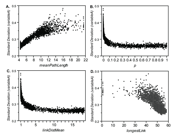
Figure 14. Standard deviation of variableA plotted against meanPathLength, p, linkDistMean, and longestLink for 3000 runs in rewireMode 1. Standard deviation is averaged over the last 500 time steps of each run.

3.20

Figure 15 shows the standard deviation of variableA plotted against MPL and linkDistMean for 4000 runs in rewireMode 2. The relationships are very similar to those produced in rewireMode 1: cultural transmission across networks with longer links and a shorter mean path length results in less variability. Figure 16 plots the standard deviation of variableA vs. p for four values of rewireRadius (2, 4, 8, and 16). As rewireRadius increases, the nonlinear relationship between p and the standard deviation of variableA becomes more apparent: small increases in p from 0 have a larger effect as the radius available for forming non-local links increases.

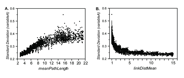
Figure 15. Standard deviation of variableA plotted against meanPathLength and linkDistMean for 4000 runs in rewireMode 2. Standard deviation is averaged over the last 500 time steps of each run. The value of rewireRadius varied randomly between 2 and 57.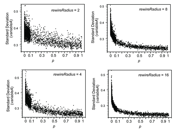

Figure 16. Standard deviation of variableA plotted against p for four values of rewireRadius (2, 4, 8, and 16), rewireMode 2.

3.21

These inter-relationships between network structure, network properties, and the standard deviation of variableA demonstrate that structured interaction affects the amount of variability generated by a simple cultural transmission process in a predictable way: networks where information flow is easier (i.e., where mean path length is low) produce less variability. This is true in both modes of network formation (compare Figure 14.A and Figure 15.A). This suggests that the properties of networks, rather than details of the structure that produces those properties, are the prime determinants of how much variability is produced.

Spatial patterning of variability

3.22

Several groups of experiments were run to evaluate how assemblage variability is structured with regard to space under different conditions of p in both modes of network formation. The Moran's I statistic was chosen to describe the degree of spatial autocorrelation among the values of variableA at the last time step in a series of experimental runs. Spatial autocorrelation is the degree to which the value of a variable at a point in space is related to the values of the same variable in adjacent points in space (seeCliff and Ord 1973; Moran 1950). Moran's I is an index: values range from +1 (perfect correlation) to -1 (perfect dispersion). A value of 0 indicates a random arrangement in space (i.e., spatial proximity has no effect on the value of a variable). Values between 0 and 1 indicate some degree of spatial clustering, where similar values are located closer to each other in space than would be expected randomly.

3.23

Moran's I was calculated on sets of model data using the Spatial Statistics tools in ArcMap 9.2. Model outputs were adjusted to produce a list containing the coordinates and value of variableA for each group at the last time step. This list was imported into GIS and converted to an XY shapefile. Moran's I was calculated on these 40 x 40 grids of data using the default settings. The XY coordinate system used for the hexagonal grid employed in the model introduces a slight distortion to the spatial relationships between agents (the Y coordinate of every other column of agents is offset by 0.5 units) when the data are read in a Cartesian coordinate system in GIS. Because this introduces only a negligible difference in Moran's I for each run, however, it has no significant effect on the analytical results and therefore no effort was made to correct this distortion.

3.24

The first of these experiments was designed to produce data to compare Moran's I to the value of p, the resulting MPL, and the resulting amount of variability in variableA at the end of runs in rewireMode 1 (Figure 17). For these 40 x 40 grids, a relatively slight deviation from 0 is a statistically significant difference from the null hypothesis of randomness. The relationship between Moran's I and p is very similar to that between p and other variables: the large majority of the variability in Moran's I within these results occurs where p < 0.10 (figure 17.a). the widest range of values of moran's i was produced when the MPL of a network was relatively high (Figure 17.B). The relationship between Moran's I and the standard deviation of variableA is relatively linear, suggesting that the degree of assemblage variability is related proportionally to the organization of variability across space (Figure 17.C). In other words, the "extra" variability that is produced through interactions when p is low is not randomly distributed across space, but is patterned in a statistically significant way.

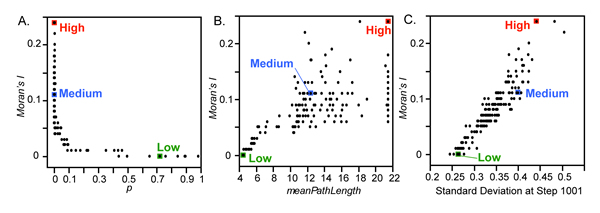
Figure 17. Relationships between Moran's I and p, meanPathLength, and the standard deviation of variableA at step 1001 for 162 runs in rewireMode 1. Individual run results marked "Low", "Medium", and "High" correspond to results shown in Figures 18 and 19.

3.25

Figure 18 shows graphic representations of example runs producing low, medium, and high values of Moran's I (designated as "Low", "Medium", and "High" in Figure 17). Data from these runs are coded using a grayscale color ramp to represent the value of variableA at the location of each group. Figure 19 depicts these same data in the form of interpolated rasters created in GIS. In the left column, the color ramps are individually calibrated to the high and low values within each grid. The rasters in the right column are displayed using a single color ramp that incorporates the full range of values present in all three grids.

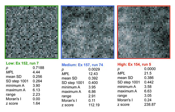
Figure 18. Results from three example runs shown with a circle shaded to represent the value of variableA for each agent.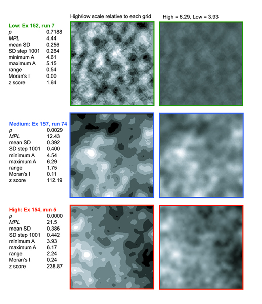

Figure 19. Rasters created in ArcGIS for the same three example runs shown in Figure 18. Rasters on the left use high and low values specific to each grid. Rasters on the right use high and low values encompassing variability in all the grids, showing both the greater amount of variability when p is low (Medium and High) and the spatial segregation of that variability.

3.26

Differences in the spatial organization of variability are apparent in these visual depictions of the data. Both the unmodified and the interpolated datasets illustrate how higher values of Moran's I are associated with increasing spatial segregation of higher and lower values of variableA. The presence of nonrandom spatial structure is linked to the much greater variability that is present in grids with high values of Moran's I.

3.27

A similar set of experiments was run to produce data on the relationships between Moran's I, p, MPL, and the standard deviation of variableA in rewireMode 2. Moran's I was calculated for datasets produced with rewireRadius set at 2 ( n =105 runs) and 8 ( n =105 runs). When the establishment of nonlocal links is limited to a single tier outside the local neighborhood (i.e., rewireRadius =2), there is no discernible relationship between p and Moran's I (Figure 20.A). Mean path lengths less than 11 are not possible (Figure 20.B). When rewireRadius =8, a nonlinear relationship between p and Moran's I is present (Figure 20.D), and MPL is positively related to Moran's I in a fashion similar to that seen in the data from rewireMode 1 (compare Figure 20.E. and Figure17.B). In both cases, the relationship between Moran's I and the standard deviation of variableA is linear, also similar to the rewireMode 1 data (Figures 20.C. and 20.F).

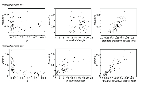
Figure 20. Relationships between Moran's I and p, meanPathLength, and the standard deviation of variableA at step 1001 for 210 runs in rewireMode 2. Top row rewireRadius = 2, bottom row rewireRadius = 8.

3.28

Because the equation-based BACE model discussed earlier does not incorporate a spatial component to interaction, the data it produces is not statistically different from random in terms of its spatial organization (i.e., Moran's I). The ACE model has no interaction structure (and therefore also no spatial component). In other words, neither of these models can be used to understand how the spatial organization of variability is related to cultural transmission when the interactions involved in that transmission have a spatial structure.

Discussion

4.1

The model has been used to produce baseline information on inter-relationships between network structure, network properties, and the outcomes of a simple cultural transmission process. It produces relationships among network properties that are consistent with the "small world" phenomenon when configured to mimic the model of Watts and Strogatz (1998). Results clearly show that the properties of the networks in the model have significant effects on both the overall amount of variability that is produced and the spatial organization of that variability. The behavior of the model suggests a set of general, directional relationships between the "rules" of network formation, the properties of the networks that are produced by those rules, and the amount and spatial organization of the variability that is produced (Figure 21). The forms these relationships take are largely a result of the nonlinear effects that the creation of relatively long nonlocal links has on network properties.

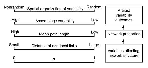
Figure 21. Conceptual summary of relationships suggested by model results.

4.2

The combinations of local and non-local ties that are present in real human networks suggest that the structures of these networks fall somewhere between the "local-only" and "random" extremes considered here. Model results suggest that the creation of a relatively sparse web of non-local connections is the most efficient way to engineer a significant improvement in the ease of information flow across a spatially-situated network like those considered here. This is true both when the model is configured to interpolate between local-only networks and random networks with no spatial constraints and when the creation of non-local connections is spatially-constrained to more closely mimic what is plausible in real human systems.

4.3

Following the relatively large reduction in mean path length that is caused by the creation of a sparse web of non-local links, the further addition of non-local links has relatively little benefit in terms of mean path length. The "cost" of establishing and/or maintaining non-local links (e.g., through travel required for face-to-face interaction, etc.) would tend to limit the creation of new links that return no added benefit. If the main purposes of maintaining non-local contacts is to facilitate "over the horizon" information flow and secure access to assistance or resources in distant areas during times of stress, the cost of maintaining connections would be an incentive to have as few as necessary to serve the purpose of maintaining sufficient information flow. While it would not increase the efficiency of information flow, however, having more than the minimum number of connections would add an element of redundancy that may be desirable under some circumstances (e.g., where the cost of network "failure" is very high). Results from the model are consistent with the idea that sparse webs of nonlocal connections produce the best trade-off between "benefit" and "cost."

4.4

Links in the model allow information to flow directly between groups, influencing the mathematical outcomes of individual copying events. In actual systems, social links between groups would function as avenues facilitating the between-group movements of people and families through marriage, individual mobility, etc. These transfers of people would change the composition of the local "pool" of information that is available. Non-local links would allow direct transfers of information (via the movements of people) between groups that are not spatially adjacent.

4.5

If we accept that many human interactions involved in cultural transmission are local (i.e., that people learn from those around them) and that human social networks are likely to be structured in some way similar to the low p networks represented by the model (i.e., largely local networks with a few non-local connections that allow movements of information between spatially-nonadjacent groups), the model data suggest that changes in the structure of interaction should be considered among the possible causes of changes in "stylistic" variability in archaeological assemblages. When the large majority of interactions are local (i.e., when p is 0 or low), relatively small changes in the number of non-local connections can have a relatively large effect on how information flows among groups and the variability of the assemblages that are produced. This suggests an appropriate "null model" for understanding the outcomes of cultural transmission processes might be one where interactions are structured through local-only networks.

4.6

Histograms of the standard deviation of variableA show that that increasing the spatial radius for adding nonlocal connections results in a greater difference in the outcomes associated with the extreme values of p (Figure 22.A and 22.B). When the radius is relatively large, the statistical patterns of variability are not substantially different than those produced when local links are simply replaced by random links (Figure 22.C).

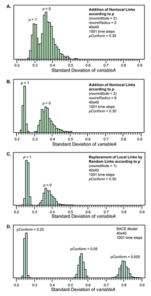
Figure 22. Histograms of outcomes (in terms of standard deviation) for p=0 and p=1 in the structured interaction model (A, B, and C) and for three settings of pConform in the BACE model (D).

4.7

Changes in the non-local component of interaction are, of course, only one potential cause of changes in assemblage variability through time. Changes in the strength of copying bias, changes in selection, and deterministic mathematical processes have all been suggested as explanations for change in archaeological assemblages (e.g., Eerkens and Lipo 2005; Hamilton and Buchanan 2009; Neiman 1995). Histograms of outcomes produced by the BACE model at various settings of pConform are shown in Figure 22.D. It is notable that, at comparable values of pConform, the BACE model produces outcomes less variable than those of a completely random network (compare the results for pConform = 0.25 in Figure 22.D with those for p=1 in Figure 22.C). A local-only interaction structure (i.e., p =0 in Figure 22.A-C) produces assemblages with more variability than assemblages produced by equation-based models that must assume random interactions or population-wide copying of mean values (neither of which actually occur in human systems).

4.8

Discerning between alternative sources of change should be a goal of future work. Independent lines of evidence are available for evaluating network-based explanations of change in variability. It is often possible to monitor changes in non-local interaction in archaeological settings through independent means such as changes in raw material use, exchange, settlement organization, etc. If there are archaeological indications of changing patterns of nonlocal interaction, we can expect that these changes may have a discernible effect on patterns of variation in realms of material culture that articulate with these interactions. Based on the model results, this is most likely to be true in cases where social networks are positioned within the "small-world" (i.e., low p) range where information flow is particularly sensitive to the addition or subtraction of small numbers of nonlocal links.

4.9

The model employed here is not intended to mimic interaction in any particular cultural system or produce data that are directly comparable to data derived from archaeological assemblages. It should be clear that the range of network structures that can be produced by the model is intended to neither include nor exhaust all possible permutations of human social networks. Network formation and maintenance "rules" other than those considered here may produce networks that have a different range of properties that are potentially important to understanding artifact variability. This model does not attempt to represent many aspects of real cultural systems that may also have a significant effect on cultural transmission and its outcomes: the interaction networks are static, all social connections are of equal strength and transmit the same information, groups are monolithic entities that do not move, style is represented as a simple "passive" quality, there is no representation of functional variability, and the geography of the world is uncomplicated.

4.10

It is exactly the abstract simplicity of models such as this one, however, that make them useful heuristic tools for generating a baseline understanding of how variables are related to one another in uncomplicated contexts. The exclusion of representations of phenomena such as agent mobility, variability in the strength and character of social connections, multi-dimensional representations of style (i.e., representing both "active" and "passive" forms of stylistic variability), network dynamics, other kinds of network structure, and complex geography ensures that these variables are not responsible for any of the behavior that the model exhibits. Aspects of network structure other than those investigated here (such as degree, for example) may also affect information flow and be related to patterns of artifact variability. Any or all of these phenomena can be represented and investigated in future models. Some of the model behavior discussed here may change when additional variables are incorporated, and some may not. A goal of future modeling work should be to evaluate which relationships are present under a variety of conditions and which are more sensitive to particular circumstances.

4.11

The usefulness of abstract models such as this one can be judged based on the model's ability to produce patterns that are expected and interpretable and its capability to contribute to the building of theory by generating specific ideas for further work (Gilbert 2008: p. 41). This model has done these things. The relationships depicted in Figure 21, while perhaps applicable to many different kinds of archaeological systems, cannot be assumed a priori to characterize any system other than that of the model. These relationships can be used as a starting point for further investigations, however. Models more specific and more complicated than the one described here will be required to generate expectations that can be compared directly to archaeological data. The voluminous ethnographic data on kinship, marriage, exchange, and mobility in hunter-gatherer systems will make it possible to create computational models useful for understanding the long-term and large-scale implications of these different behaviors in terms of network structure, network properties, and patterns of artifact variability (cf. White and Johansen 2005).

Conclusion

5.1

This paper adds additional elements to the basic view that differences in how information is transferred in a cultural system might have outcomes that we can observe in patterns of variability in material culture. Cultural transmission provides a point of articulation between social networks and material culture. Agent-based modeling allows us to investigate how macro-level patterns of variability are affected by the rules governing individual interactions in complex, network-mediated, spatially-situated systems. The model described here shows that the spatial structure of interaction has patterned effects on artifact variability that are potentially significant and comparable in magnitude to those of "copying bias." The assumption of unstructured information transfer that is fundamental to equation-based models is neither a reasonable simplification nor an analytical necessity. The structure of interaction makes a difference to the outcomes of cultural transmission processes and should be considered a potentially important causal factor.

5.2

Understanding how network structure affects the transfer of information and the resulting time-space patterns of variability may help us understand the complex, multi-dimensional patterning that is characteristic of so many aspects of modern human systems. If the "natural" outcome of open, local-only networks is to produce regionalized or clinal patterns of variability, this may go some distance towards explaining the macro-fragmentation described by Yellen and Harpending (1972) and the non-isomorphic distributions of language, biological variation, and different aspects of material culture that are notable feature of many human cultural systems (e.g., Boas 1911; Hymes 1967). Information transfer in each of these domains may take place largely at the level of localized interactions between individuals, mediated through social networks. The non-linear behaviors of network-mediated systems could also shed light on the variable rates and dimensions of change across time and space which are a characteristic aspect of the prehistoric archaeological record (cf. Ramsey 2003; Schiffer and Skibo 1987; Shott 1996, 2008).

Acknowledgements

This paper is a step in an ongoing effort to use computational modeling to understand the complex relationships between social network structure and material culture in hunter-gatherer systems. I am grateful for the continuing encouragement and support of Rick Riolo, John Speth, Bob Whallon, and Henry Wright at the University of Michigan, and to other faculty and students who have taken an interest in this work and braved the consequences of initiating a discussion about it. The modeling work described in this paper was conducted at the Center for the Study of Complex Systems at the University of Michigan. I thank John Speth and Rick Riolo for providing valuable feedback on early drafts of this paper. All errors and weaknesses remain the sole property of the author.

References

AXELROD, R. (1997). The dissemination of culture: a model with local convergence and global polarization. The Journal of Conflict Resolution, 41(2), 203-226. [doi:10.1177/0022002797041002001]

BAMFORTH, D.B., Finlay, N. (2008). Introduction: archaeological approaches to lithic production skill and craft learning. Journal of Archaeological Method and Theory, 15, 1-27. [doi:10.1007/s10816-007-9043-3]

BANKS, W.E., Zilhao, J., d'Errico, F., Kageyama, M., Sima, A., Ronchitelli, A. (2009). Investigating links between ecology and bifacial tool types in Western Europe during the Last Glacial Maximum. Journal of Archaeological Science, 36, 2853-2867. [doi:10.1016/j.jas.2009.09.014]

BARNES, J.A. (1972). Social Networks. Addison-Wesley Module in Anthropology, Module 26. Reading, Massachusetts: Addison-Wesley Publishing Company.

BENTLEY, R.A., Shennan, S.J. (2003). Cultural transmission and stochastic network growth. American Antiquity, 68(3), 459-485. [doi:10.2307/3557104]

BERRY, J.W., Georgas, J. (2009). An ecocultural perspective on cultural transmission: the family across cultures. In Schonpflug, U., (Ed.), Cultural Transmission: Psychological, Developmental, Social, and Methodological Aspects (pp. 95-126). Cambridge: Cambridge University Press.

BETTINGER, R.L., Eerkens, J. (1999). Point typologies, cultural transmission, and the spread of bow-and-arrow technology in the prehistoric Great Basin. American Antiquity, 64(2), 231-242. [doi:10.2307/2694276]

BLAU, P.M., Scott, W.R. (1962). Formal Organizations: A Comparative Approach. San Francisco: Chandler Publishing Company.

BOAS, F. (1911). Introduction. In Handbook of American Indian Languages (pp. 1-83). Washington, D.C.: Bureau of American Ethnology.

CLIFF, A.D., Ord, J.K. (1973). Spatial Autocorrelation. London: Pion Limited.

CONKEY, M.W. (1980). Context, structure, and efficacy in Paleolithic art and design. In LeCron, M., Brandes, S.H. (Eds.), Symbol as Sense (pp. 225-248). New York: Academic Press.

EERKENS, J.W. (2000). Practice makes within 5% of perfect: visual perception, motor skills, and memory in artifact variation. Current Anthropology, 41, 663-667. [doi:10.1086/317394]

EERKENS, J.W., Lipo, C.P. (2005). Cultural transmission, copying errors, and the generation of variation in material culture and the archaeological record. Journal of Anthropological Archaeology, 24, 316-324. [doi:10.1016/j.jaa.2005.08.001]

GAMBLE, C. (1986). The Palaeolithic Settlement of Europe. Cambridge: Cambridge University Press.

GILBERT, N. (2008). Agent-Based Models. Quantitative Applications in the Social Sciences 153. Thousand Oaks, California: Sage Publications.

HAMILTON, M.J., Buchanan, B. (2009). The accumulation of stochastic copying errors causes drift in culturally transmitted technologies: quantifying Clovis evolutionary dynamics. Journal of Anthropological Archaeology, 28, 55-69. [doi:10.1016/j.jaa.2008.10.005]

HYMES, D.H. (1967). Linguistic problems in defining the concept of "tribe." In Helm, J. (Ed.), Essays on the Problem of Tribe (pp. 23-48). Seattle: University of Washington Press.

ISAAC, G.L. (1972). Early phases of human behaviour: models in Lower Palaeolithic archaeology. In Clarke, D.L. (Ed.), Models in Archaeology (pp. 167-199). London: Metheun & Co.

KEMPE, M., Lycett, S., Mesoudi, A. (2012). An experimental test of the accumulated copying error model of cultural mutation for Acheulean handaxe size. PLoS One, 7(11), e48333. [doi:10.1371/journal.pone.0048333]

KLEMM, K., Eguíluz, V.M., Toral, R., Miguel, M.S. (2003). Nonequilibrium transitions in complex networks: a model of social interaction. Physical Review E, 67 026120, 1-6. [doi:10.1103/physreve.67.026120]

KOLDEHOFF, B., Loebel, T.J. (2009). Clovis and Dalton: unbounded and bounded systems in the midcontinent of North America. In Adams, B., Blades, B.S. (Eds.), Lithic Materials and Paleolithic Societies (pp. 270-287). West Sussex: Wiley-Blackwell. [doi:10.1002/9781444311976.ch20]

LOVEJOY, W.S., Loch, C.H. (2003). Minimal and maximal characteristic path lengths in connected sociomatrices. Social Networks, 25, 333-347. [doi:10.1016/j.socnet.2003.10.001]

MINAR, C.J. (2001). Motor skills and the learning process: the conservation of cordage final twist direction in communities of practice. Journal of Anthropological Research, 57(4), 381-405.

MINAR, C.J., Crown, P.L. (2001). Learning and craft production: an introduction. Journal of Anthropological Research, 57(4), 369-380.

MORAN, P.A.P. (1950). Notes on continuous stochastic phenomena. Biometrika, 37, 17-23. [doi:10.1093/biomet/37.1-2.17]

NEIMAN, F.D. (1995). Stylistic variation in evolutionary perspective: inferences from decorative diversity and interassemblage distance in Illinois Woodland ceramic assemblages. American Antiquity, 60(1), 7-36. [doi:10.2307/282074]

NEWMAN, M.E.J. (2000). Models of the small world. Journal of Statistical Physics, 101, 819-841. [doi:10.1023/A:1026485807148]

PREMO, L.S., Scholnick, J.B. (2011). The spatial scale of social learning affects cultural diversity. American Antiquity, 76(1), 163-176. [doi:10.7183/0002-7316.76.1.163]

RADCLIFFE-BROWN, A. R. (1940). On social structure. Journal of the Royal Anthropological Institute, 70, 1-12. [doi:10.2307/2844197]

RAMSEY, C.B. (2003). Punctuated dynamic equilibria: a model for chronological analysis. In Bentley, R.A., Maschner, H.D.G. (Eds.), Complex Systems and Archaeology (pp. 85-92). Salt Lake City: The University of Utah Press.

SCHIFFER, M.B., Skibo, J.M. (1987). Theory and experiment in the study of technological change. Current Anthropology 28(5), 595-622. [doi:10.1086/203601]

SHENNAN, S.J., Steele, J. (1999). Cultural learning in hominids: a behavioural ecological approach. In Box, H.O., Gibson, K.R. (Eds.), Mammalian Social Learning: Comparative and Ecological Perspectives (pp. 367-388). Cambridge: Cambridge University Press.

SHOTT, M.J. (1996). Innovation and selection in prehistory: a case study from the American Bottom. In Odell, G. (Ed.), Stone Tools: Theoretical Insights into Human Prehistory (pp. 279-309). New York: Plenum Press. [doi:10.1007/978-1-4899-0173-6_11]

SHOTT, M.J. (2008). Darwinian evolutionary theory and lithic analysis. In O'Brien, M. (Ed.), Cultural Transmission and Archaeology: Issues and Case Studies (pp. 146-157). Washington, D.C.: SAA Press.

STARK, M.T., Bowser, B.J., Horne, L. (Eds.). (2008). Cultural Transmission and Material Culture. Tucson: University of Arizona Press.

WATTS, D.J., 2004. The "new" science of networks. Annual Reviews of Sociology, 30, 243-270. [doi:10.1146/annurev.soc.30.020404.104342]

WATTS, D.J., Strogatz, S.H. (1998). Collective dynamics of "small-world" networks. Nature, 393, 440-442. [doi:10.1038/30918]

WHITE, A.A. (2006). A model of Paleoindian hafted biface chronology in northeastern Indiana. Archaeology of Eastern North America, 34, 29-59.

WHITE, A.A. (2012). The Social Networks of Early Hunter-Gatherers in Midcontinental North America. Unpublished Ph.D. dissertation: University of Michigan.

WHITE, D., Johansen, U. (2005). Network Analysis and Ethnographic Problems: Process Models of a Turkish Nomad Clan. Lanham: Lexington Books.

WOST, H.M. (1974). Boundary conditions for Paleolithic social systems: a simulation approach. American Antiquity, 39(2), 147-178. [doi:10.2307/279579]

WOBST, H.M. (1976). Locational relationships in Paleolithic society. Journal of Human Evolution, 5, 49-58. [doi:10.1016/0047-2484(76)90099-3]

WOBST, H.M. (1977). Stylistic behavior and information exchange. In Cleland, C. (Ed.), Papers for the Director: Research Essays in Honor of James B. Griffin (pp. 317-342). Anthropological Papers 61. Ann Arbor: University of Michigan Museum of Anthropology.

YELLEN, J., Harpending, H. (1972). Hunter-gatherer populations and archaeological inference. World Archaeology, 4(2), 244-253. [doi:10.1080/00438243.1972.9979535]