
 Abstract
- To explore the minimization of the marketing cost and the maximization of the user perceived utility, an optimization model for mobile banking adoption with incomplete information is developed. A combination of qualitative simulation and empirical study can serve as a solution to the optimization problem. Firstly, we use mobile banking system as an example with questionnaire designed to obtain data from customers, which is then statistically analyzed using SPSS to examine the interactions among adoption drivers. Secondly, a qualitative simulation method is introduced to drive the evolution of the interactions among these adoption drivers. Thirdly, according to the empirical relations, an optimization model is established, and the objective functions are examined by the BP neural network. Then, to examine the feasibility of the framework, a prototype system based on MATLAB is implemented. It is found that the results are consistent with common sense (oscillation-equilibrium theory), and the framework is able to contribute to real-time optimization decision supports in the mobile banking marketing. In practice, the identification of the optimal combination of change directions can serve as the development priorities in adoption drivers, and is likely to influence resource allocation in the future mobile banking development.
- Keywords:
- Mobile Banking Adoption, Optimization, QSIM, Empirical Study, BP Neural Network
Introduction
- 1.1
- M-banking service has been increasingly deployed by modern banks because of its low cost and convenience. In China, with the accelerating pace of 3G, m-banking has recently spread at all levels. However, compared with a large number of cell phone users who are regarded as potential adopters, m-banking adoption has been limited and even, in many cases, has fallen short of expectations. The adoption rate of mobile netizens in China was up to 52.2% in February 2011 compared with 36.8% in July 2010 (3G Portal 2011). Although m-banking adopters significantly increased by 150% from 2010 to 2011 and approximately 93% of customers had a bank account, only 25% of consumers adopted m-banking as their primary banking channel (TNS 2011). Compared with users of offline channels, the number of m-banking adopters is far from adequate. Therefore, some measures are necessary for banks to promote m-banking adoption.
- 1.2
- According to whether they are directly related to banks or customers, the advantages of m-banking adoption can be placed into two overarching categories (Xue et al. 2011). First, m-banking reduces service costs. The cost of an account transfer is approximately $1.07 through a branch and $0.27 at an ATM but is only $0.01 through m-banking (Chang 2002). Second, compared with offline channels, customers adopting m-banking are more likely to experience a higher perceived utility (Hitt et al. 2002; Gerrard et al. 2003). For instance, the convenience of m-banking will improve customer utility. This paper explores how to minimise marketing costs and maximise perceived customer utility with incomplete information.
- 1.3
- The existing literature on online banking adoption seldom involves real-time optimisation; it has principally focused by survey method on social and technical dimensions such as perceived usefulness towards the variations in m-banking adoption (Chase 1978; Chase 1981; Chatterjee et al. 1990; Chen et al. 2002; Choi et al. 2010). However, there were at least two significant limitations. First, such studies are typically limited to a single time period and thus cannot examine the dynamic interaction among determinants such as the feedback effects from banking, cost factors or customer utility factors. Second, continuous collection of data is quite difficult, as it is both time consuming and costly (Davis et al. 1989; Davis 1989). For instance, if the external environment and the object of study change, the model must be rebuilt and rerun, and the parameters of the empirical model must be modified. Thus, an empirical model is not appropriate for an optimisation problem in adoption behaviour, especially with incomplete information.
- 1.4
- In this paper, the integrated framework for optimization problem in m-banking adoption has been proposed. Although qualitative simulation is inaccurate, the combination of qualitative simulation and empirical study can solve the optimization problem with incomplete information. Specially, this empirical study was introduced to examine the interaction among adoption drivers. Second, this qualitative simulation method was adopted to drive the evolution of the empirical relations. Third, according to the empirical result, the optimization model was established, and the objective functions were examined by BP neural network. Finally, the prototype system based on MATLAB was implemented, and the feasibility of our model was validated.
Literature Review
- 2.1
- Our study is directly related to the diffusion of technology and innovation, especially of online banking services (Davis et al. 1989; Karjaluoto et al. 2002; Gerrard et al. 2003; Gefen et al. 2003), most of which are based on the Bass model. The well-known Bass model first proposed that aggregate product adoption is associated with product attributes and adopters' quantity. Scholars then extended the perspective on adoption behaviour from aggregate adoption to individual adoption decisions (Purnima et al. 2011) and showed that market-wide factors (total adoption), customer characteristics, and service characteristics affect product adoption.
- 2.2
- A substantial body of literature has utilised network externalities to investigate the effect of existing adopters on future adoption. It has been determined that not only customer demographic characteristics but also the number of existing customers in the same geographic region have a significant effect on individual adoption behaviour (Goolsbee et al. 2002). The technology acceptance model (TAM) investigated the interaction between individual characteristics and technology diffusion and revealed the manner in which individual characteristics affect technology adoption behaviour (Davis et al. 1989; Davis 1989).
- 2.3
- In addition, the correlation between online banking adoption and future performance has been examined. Scholars further investigated the effect of adoption behaviour on customer profitability in the long term, indicating that online banking adopters are likely to accrue more profit both before and after their adoption behaviour (Hitt et al. 2002). Recent literature showed that customer characteristics have a negative effect on profitability and that adoption behaviour is associated with the market share of banks (Campbell et al. 2010). Our work is also closely related to the existing literature that studied the aggregate effects of adoption behaviour, including product diffusion, local penetration, availability of alternatives, and individual characteristics (Xue et al. 2011). Using panel data, drivers and outcomes of online banking adoption were explored to determine the value of an online banking channel.
- 2.4
- In summary, existing literature has focused on product diffusion, network effects and TAMs to examine adoption behaviour. Most of these studies were based on survey data and focused on modelling the correlation between customer demographics and online banking diffusion. Other factors that were considered include technological expertise (e.g., customers' prior computer experience or experience with other similar technologies), convenience, desire to use innovative products, security, privacy, and trust (Purnima et al. 2011).
- 2.5
- Our paper extends these literature streams to the optimization field, which is uncommon in them. To solve the optimization problem with incomplete information, an integrated paradigm that combines qualitative simulation and empirical method was proposed. In details, by using qualitative simulation, we were not subjected to a single time period and thus could examine the evolution of interactions among adoption drivers. Next, the empirical method was utilized to obtain the causality among adoption drivers in uncertain environment. Our experimental results proved the feasibility of the integrated paradigm.
Empirical model on m-banking adoption
- 3.1
- The random utility theory (McFadden 1974) examined the reason for online banking adoption and revealed that people are more likely to adopt a product with high utility and low costs. We chose the factors directly influencing bank costs and customer utility as constructs in this paper. Technology Acceptance Model (denoted as "TAM") introduced perceived usefulness (PU), perceived ease of use (PE), usage attitude (UA) and usage intention (UI) as primary adoption drivers. These internal control factors, which refer to customer utility, are characteristics of the individual. TAM has been widely accepted and expanded. Theory of planned behaviour, as one predictive persuasion theory, studies the relations among beliefs, attitudes, behavioural intentions and behaviours. The theory of planned behaviour (denoted as "TPB") focuses on the external factors that influence adoption behaviour. These factors depend on the situation, which refers to the bank costs (Davis et al. 1989). Business reputation (BR) perceived risk (PR), subjective norms (SN) and perceived behavioural control (PBC) from the TPB were added to the original TAM and deemed to be important adoption drivers (Purnima et al. 2011). Accordingly, we chose PU, PE, PR, BR, UA, SN, PBC and UI as constructs in our model.
Hypotheses
- 3.2
- Usefulness and Ease of Use: Links between perceived usefulness, ease of use, intention and attitude in the TAM theory have been empirically verified. Perceived ease of use has a significant effect on perceived usefulness (Bruner et al. 2005). The TAM also examined the correlation between individual characteristics and technology diffusion, which identified usefulness as an important adoption driver (Davis et al. 1989; Davis 1989). Customers tend to adopt m-banking with more usefulness. Finally, we propose that behavioural attitudes are determined by perceived usefulness and ease of use in the TAM model because the psychological discomfort and anxiety from less ease of use would devalue perceived usefulness. Attitude refers to a person's perception of m-banking. The TAM holds that the actual adoption of a system depends on a customer's adoption intention and is ultimately determined by usage attitude (Davis 1989).
H1: Higher ease of use is associated with higher usefulness.
H2: Higher usefulness is associated with higher attitude.
H3: Higher usefulness is associated with higher intention.
H4: Higher ease of use is associated with higher attitude.
H9. Attitude has a positive effect on adoption intention.
- 3.3
- Perceived Risk: Perceived Risk refers to the threats that cause economic hardship to data or network resources in the form of destruction, disclosure, modification of data, denial of service and/or fraud, waste, and abuse (Gefen et al. 2003). Particularly in m-banking, perceived risk is associated with spyware, phishing attacks, mobile phone viruses, anti-DDoS protection and application vulnerability. Security risk is a significant impediment to the adoption of online banking (Milind 1999). Perceived risk has an effect on adoption attitude (Dowling et al. 1994).
H5: Higher levels of perceived risk are associated with reduced adoption attitude.
- 3.4
- Reputation: Reputation refers to the adopters' beliefs in transaction security and privacy protection. Because of the spatial and temporal separation of customers and mobile banks, the trust between these entities appears to be important. When customers perform an online transaction, their personal information (e.g., bank account, and password) is disclosed to banks (Chen et al. 2002). Therefore, mobile banks with good reputations will win customer trust in m-banking transactions, and finally influence the usage attitude.
H6: Higher levels of perceived reputation are associated with increased attitude.
- 3.5
- The TPB examines the external adoption drivers depending on the situation, and indicates that both subjective norms and perceived behavioural control shape the adoption intention.
- 3.6
- Subjective Norms: Subjective Norm refers to the perceived pressure from other individuals (e.g., colleagues and friends) to adopt a system. When customers have less online banking experience, their beliefs will be significantly affected by the opinions of others. In addition, the perceived security of m-banking adoption will be improved by the normative pressure from reference groups. Accordingly, these norms are identified as an important adoption driver.
- 3.7
- Perceived Behavioural Control: Perceived behavioural control indicates the perception of the difficulty in adopting m-banking and refers to the beliefs about having the necessary resources and opportunities to adopt m-banking (Davis et al. 1989). The TPB hold that adoption intentions are determined by perceived behavioural control. Hence, the direct effect of perceived behavioural control on adoption intention will be tested by the following hypotheses:
H7: Higher subjective norms are associated with increased adoption intentions.
H8: Perceived behavioural control has a positive effect on adoption intentions.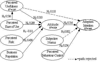
Figure 1. Path analysis result based on all valid samples (n=369) Research methodology
Measurement
- 3.8
- Based on an intensive literature review, a measurement scale of relation strength in the context of m-banking adoption was developed and validated. A seven-point Likert-scale ranging from strongly disagree-(1) to strongly agree-(7) was used to measure each scale item. For statistical analysis, the program SPSS 16.0 was used. In our empirical study, respondents were recruited from Huazhong University of Science and Technology, involving undergraduate and graduate majoring arts and science. From the perspective of educational background and age, the sample collection investigated can reflect characteristics of all banking customers in the region. And 250 questionnaires were sent out, receiving 234 efficient questionnaires with 93.6% retrieving rate, of which 224 valid questionnaires were got with an effective rate of 95.7%.
Reliability and validity of the measurement model
- Reliability analysis
Before the further analysis, reliability analysis was performed by Cronbach's Alpha and composite reliability (CR). Cronbach's Alpha, as a coefficient of internal consistency, was utilized to assess the reliability of scales. The internal consistency was further examined by CR to test the stability of the individual measurement items. Cronbach's alpha and CR all well exceeded the recommended value level of 0.8 (Gefen et al 2003; Straub 1989), which revealed adequate reliability of the factors (see Table 1).
Table 1: Measurement items and reliability Measurement item AVE Alpha FL CR Perceived Usefulness (PU) 0.646 0.816 0.879 PU1: M-banking provides service that I need 0.785 PU2: Information that m-banking provide is accurate and credible 0.869 PU3: I think m-banking service is very helpful to my life in general 0.803 PU4: M-banking adoption is useful for managing my finances 0.754 Perceived Ease of Use (PE) 0.711 0.797 0.880 PE1: My interaction with m-banking is clear and understandable 0.758 PE2: M-banking adoption is easy and convenient 0.888 PE3: Learning to use the m-banking would be easy 0.877 Perceived Risk (PR) 0.689 0.863 0.898 PR1: I feel adopting m-banking in monetary transactions is risky 0.840 PR2: I feel fraud and abuse in m-banking is risky 0.779 PR3: I feel erroneous operation in m-banking adoption is risky 0.859 PR4: I feel adopting m-banking would divulge my personal information 0.840 Business Reputation (BR) 0.724 0.809 0.887 BR1: I believe m-banking are trustworthy 0.887 BR2: I believe the bank will consider customers' profit as top priority 0.810 BR3: I believe the banks will keep its promises and commitments 0.810 Usage Attitude (UA) 0.777 0.852 0.913 UA1: I think that m-banking adoption is good idea 0.880 UA2: I think that m-banking adoption is beneficial to me 0.899 UA3: I have positive perception about m-banking adoption 0.865 Subjective Norms (SN) 0.641 0.729 0.840 SN1: People who influence my behavior think I should adopt m-banking 0.855 SN2: People who are important to me think I should adopt m-banking 0.875 SN3: Mass media often promotes me to adopt m-banking 0.652 Perceived Behavior Control (PBC) 0.869 0.850 0.930 PBC1: I adopt m-banking if it would be easy to access 0.940 PBC2: I adopt m-banking if I feel it is worthwhile to me 0.924 Usage Intention (UI) 0.784 0.859 0.916 UI1: I intend to adopt m-banking continuously in the future 0.910 UI2: I intend to adopt m-banking as much as possible 0.911 UI3: I recommend others to use m-banking 0.833 - Validity analysis
Due to the measurement error, the validity of all the items should be examined. The Kaiser-Meyer-Olkin measure of sampling adequacy was utilized to determine the appropriateness of factor analysis, by testing the correlation coefficient between variables. Factor analysis cannot be used if the Kaiser-Meyer-Olkin value is below 0.5 (Kaiser, 1974). The Kaiser-Meyer-Olkin measure of sampling adequacy was 0.866, confirming the applicability of factor analysis. Furthermore, the Bartlett test can be used to verify that variances are equal across groups or samples. Bartlett's test of sphericity (significance < 0.001) favored the rejection of null hypothesis that the variables with each dimension are uncorrelated in the population.
Construct validity include convergent validity and discriminate validity (Straub 1989). We tested convergent validity by average variance extracted (AVE). The AVE were all well above the recommended value level of 0.50 (see Table 1). Furthermore, convergent validity was also demonstrated by factor loading of the measurement items (Purnima et al. 2011). Almost all of the factor loadings (FL) exceeded 0.80 (see Table 1), which suggested adequate convergent validity.
In general, discriminant validity is satisfactory when AVE from the construct is greater than the variance shared between the construct and other constructs. The square root of AVE on the diagonal was greater than correlations among constructs (see Table 2). For further discriminant validity, the exploratory factor analysis was performed (see Table 3). Factor loadings obtained using varimax rotation exceeded the cut-off point 0.6 (Purnima et al. 2011).
Table 2: Discriminant validity and correlations of constructs PE PU UA UI PR BR PBC SN PE 0.843 PU 0.536 0.804 UA 0.588 0.630 0.881 UI 0.507 0.525 0.646 0.885 PR -0.131 0.005 -0.103 -0.133 0.830 BR 0.454 0.476 0.673 0.466 0.076 0.851 PBC 0.330 0.455 0.509 0.518 0.017 0.392 0.932 SN 0.399 0.543 0.526 0.443 0.044 0.390 0.353 0.801 Table 3: Rotated component matrix Component emerged Ease of Use Perceived
UsefulnessPerceived
RiskBusiness
ReputationUsage
AttitudeSubjective
NormsBehavior
ControlUsage
IntentionPE2 0.794 PE3 0.894 PE4 0.844 PU1 0.802 PU2 0.860 PU3 0.783 PU4 0.770 PR1 0.717 PR2 0.868 PR3 0.910 PR4 0.876 BR1 0.877 BR2 0.815 BR3 0.860 UA1 0.863 UA2 0.904 UA3 0.878 SN1 0.826 SN2 0.833 SN3 0.761 PBC1 0.932 PBC2 0.932 UI1 0.895 UI2 0.912 UI3 0.850
Hypotheses testing and discussion of results
- Reliability analysis
- 3.9
- The path coefficients from the model analysis are shown in Figure 1. H1, H2, H3 and H9 examine the causality shown in original TAM. Similar to TAM, the effect of perceived attitude on perceived intention is significant ( β =0.516, p <0.01). both perceived usefulness (pu) (β =0.310, p <0.001) and perceived ease of use (β =0.209, p <0.01), in turn, are also found to be determinants of perceived attitude. h5 (β=-0.111, p <0.01) and h6 (β=0.439, p <0.01) reveal that the causalities from perceived risk and business reputation on perceived attitude both are significant. no significant causality between ease of access and intention is supported (h7:β =0.882, p >0.01). However, the positive effect from behavioral control on perceived intention is proved (H8: β =0.225, p <0.01).
- 3.10
- Altogether, perceived usefulness, perceived ease, perceived risk and business reputation accounted for 62.4 percent of the variance in usage attitude, with business reputation contributing more to intention than any other construct (see Figure 2). Usage attitude accounts for 46.6 percent of the variance in usage intention. In addition, we performed path analysis in the original TAM model based on the same samples. In the study of TAM, the variance in usage attitude and usage intention is explained by 49.9 and 44.2 percent respectively. Compared with the studies of the TAM, the findings of this revised model have a greater ability to predict and explain the behavioral intention to adopt m-banking.
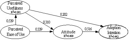
Figure 2. Path analysis result in TAM model
Optimisation Design
-
Problem Description
- 4.1
- Despite the recent rapid development of m-banking in China, the number of m-banking adopters is far from adequate. Therefore, improvement is necessary for banks and other financial institutions to promote m-banking, especially with the constraint of marketing costs. M-banking is preferable to offline channels for two reasons. First, from a transaction cost perspective, most modern banks deploy m-banking capabilities to reduce costs while improving customer service (Xue et al 2011). Second, from a utility perspective, customers choose the product that offers them the highest utility given the relative costs (McFadden 1974). M-banking adoption indicates utility-enhancing behaviours (e.g., increased usefulness). Thus, the optimisation problem can be summarised as follows: at some time point, how to improve adoption drivers to maximise the perceived utility of customers and minimise the promotion costs of mobile banks.
Variables and Optimisation model
- 4.2
- Seven adoption drivers were examined in the empirical model. According to whether they are influencing marketing costs or perceived utility directly, these variables can be placed into two overarching categories: customer utility variables and bank cost variables. The utility variables refer to a customer's perception of m-banking value, whereas the cost variables refer to a bank's marketing expenses for m-banking promotion. Customers are more likely to adopt m-banking with higher utility, and marketing expenses enable banks to prevent customer churn. If X is utility variables, then X ={ X1, X2, X3, X4 }={usefulness, ease of use, attitude, willingness}. If Y is cost variables, then Y ={ Y1, Y2, Y3 }={perceived risk, business reputation, perceived behaviour-control}. Let Z ={ X, Y } in which Z refers to adoption drivers.
Qualitative state description
- 4.3
- Qualitative value is expressed by two aspects: "level" and "change direction" (Kuipers 1993). The qualitative value of Z at time point tm and in time interval ( tm, t m+1) is expressed as QS( Z, tm) and QS( Z, tm, t m+1), respectively. Define state variables Z as

(1) in which qval and qdir indicate the magnitude and the change direction of Z, respectively. A time point tm indicates that Z changes at a distinguished time point, and tm ∈{ t0, t1, …, tn } is a distinguished time point. When a qualitative model runs, the simulation clock is moved alternately between the time point and the time interval, which are defined as different time stages. Thus, the time stages are expressed by t0, (t0, t1), t1, (t1, t2)… t m-1, (tm-1, tm), tm. qval are specified as follows:

(2) in which lk indicates the landmark value of Z, and ( lk,, l k+1) indicates that the magnitude of factors qval is between lk and l k+1.
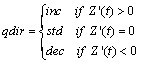
(3) Here inc, std and dec denote a change direction of Z, inc, dec and std indicates "increase", "decrease" and "standard" (no change) respectively. For more details on QSIM see Kuipers (1986).
- 4.4
- For example, to describe the temperature change of a glass of water, more than two landmark values are introduced: 0°C and 100°C. In detail, 0 is the initial temperature, and 100 is the temperature of the boiled water. By the qualitative description method, the process by which the water is heated to boiling can be described as QS (water temp, now) = <(0°c, 1000°c), inc>.
Variables
- 4.5
- Historically, the levels of state variables include "low", "moderate" and "high", and the change direction is expressed in three ways: "decrease", "standard" or "increase". For more accuracy and reliability, we improved the conventional description method. The level and the change direction of a state variable are denoted as follows:
- 4.6
- For the level of the state variables Z, k∈{1,2,…,5}, lk refers to the following:
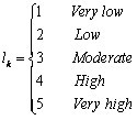
(4) in which "1", "2", "3","4" or "5" indicates that the level of a variable is very low, low, moderate, high or very high, respectively. For example, qval(X1, tm)=1 indicates that the level of perceived usefulness is very low at tm, and qval(Y1, tm)=5 indicates that m-banking is highly risky at tm.
- 4.7
- The change direction qdir of a state variable Z is expressed as
(5) in which qdir includes two aspects: "change direction" and "change degree". In details, "-1", "-0.5", "0", "0.5" and "1" indicate that the change is "decreases with a high degree", "decreases with a low degree", "no change", "increases with a low degree" and "increases with a high degree". For example, QS( Y1, tm, t m+1) = <(3,4), -0.5> shows that the level of risk is between moderate and high in time interval ( tm, t m+1) and will decrease with a low degree. QS( X1, tm) = <2, +> shows that the level of usefulness is low at tm and will increase with a high degree.
Optimisation model
- 4.8
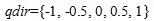
- Based on the description method above, we built an optimisation model for adoption behaviour. As the banks adapt, each change combination of adoption drivers has two certain performance scores, which refer to the utility function F and the cost function G. The objective of m-banking adoption is to maximise customer utility and minimise bank costs. The multi-objective optimisation model with initial state constraints is shown as follows:
(6) Here F as the function of utility variables represents customer utility and G as the function of cost variables expresses bank costs. X and Y indicate utility variables and cost variables, xi and yj show the initial level (magnitude) of adoption drivers, and dirxi and diryj mean the change direction.
Objective function
- 4.9
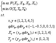
- To predict bank costs and customers' utility, a neural network was introduced to serve as the utility function F and cost function G. Recently efforts have been made to apply the neural network method to forecasting decision-making performance in the management field. The widely used BP neural network, was utilised as our forecasting model. Neural network training refers to selecting the network parameters to minimise the fitting error for a sampling set (see Figure 3). Let customer utility F(X)∈(-1,1) and bank cost G(Y)∈(-1,1). In this section, X and Y are supposed to be input vectors of the sample in a training set, whereas F(X)and G(Y)are the network output vectors of the training sample. The objective functions ( F and G) can be represented by the neural network with good convergence.
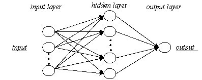
Figure 3. BP neural network trained as functions - 4.10
- The samples for training X are shown in Table 4: (1) At the initial state QS( X, t0), customers are accustomed to the internal and external environment. Thus, the perceived utility is supposed to be at a moderate level ( F(X)=0.5). Then let QS( X, t0) be an input vector, and F(X)=0.5 be an output vector. (2) As shown in the empirical research, the utility variables including perceived usefulness ( X1), ease of use ( X2), attitude ( X3) and willingness ( X4) are positively associated with usage behaviour. Thus, we suppose that utility variables with very high levels ( qval =5) enable the highest utility ( F(X)=1) whereas utility variables with very low levels ( qval =1) enable the lowest utility ( F(X)=-1). Then let the two groups of vectors be samples in the training set. Similarly, we define the samples used for training Y (see Table 5).
Table 4: The samples used for training X X1 X2 X3 X4 F(X) QS(X1,t0) QS(X2,t0) QS(X3,t0) QS(X4,t0) 0.5 5 5 5 5 1 1 1 1 1 -1 Table 5: The samples used for training Y Y1 Y2 Y3 G(Y) QS(Y1,t0) QS(Y2,t0) QS(Y3,t0) 0.5 1 5 5 1 5 1 1 -1
Qualitative Simulation Methods
- 5.1
- Traditionally, a quantitative approach was utilized to deal with the optimization problem. However, in management fields especially on the adoption behavior problems, individuals make decision not based on perfect numerical information but on information that is empirical or qualitative. Thus, a traditional quantitative approach is no longer available. A new paradigm (a combination of qualitative simulation and empirical study) was introduced to solve the optimization problem with ambiguous, incomplete or qualitative information. In details, the empirical relation between adoption divers (see Figure 1) was utilized to serve as causal graph in qualitative simulation, where causality weights was represented by the path coefficient from empirical research. Then the evolution between adoption drivers was examined by QSIM algorithm. Then, the solution to qualitative optimization problem can be obtained.
Adoption Behaviour Causality
- 5.2
- In prior qualitative simulation methods, dynamic interaction between variables was investigated by the combination of QSIM with a basic causal graph. However, the basic causal graph seems to be somewhat simple when facing complex problems in management fields. QSIM should be integrated with a more comprehensive causal reasoning method (Cem Say and Akyn 2003). For more accuracy, we utilised empirical correlations (see Figure 1) to represent a basic causal graph in a qualitative simulation in which the causality weights are expressed by a path coefficient in the empirical study.
- 5.3
- The interaction among adoption drivers results in the evolution of adoption behaviour. The utility variables refer to the internal environment, whereas the cost variables refer to the external environment. As shown in Figure 4, at time point tm , the cost variables have an effect on customer utility, and the perceived utility of customers has a simultaneous feedback loop (see W in Figure 4). At the time point t m+1, the customer's perceived utility variables have an adverse feedback effect on bank cost variables (see W' in Figure 4). Therefore, it is the alternating effects that drive the evolution of adoption behaviour.
Figure 4. M-banking adoption model - 5.4
- The causal reasoning method has been widely used in the field of economics. By creating a causal ordering graph, the modelling of economic systems, financial reporting and voluntary disclosure was explored (Berndsen et al 1994; Berndsen 1995; Koonce et al 2011). In this paper, a basic causal graph (see Figure 5) was utilised to represent the interaction among adoption drivers. A is the cause variable, and B is the effect variable. tm is the time point when A begins to affect B. ( tm, t m+1) is the time interval in which B changes gradually. t m+1is the time point when the change of B has been completed. D represents the effect of A on B, D ∈ {-, 0, +}. For example, "+" indicates that A has a positive effect on B.
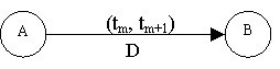
Figure 5. Basic causal graph - 5.5
- The changes of A will have an effect on B. If the change direction of A is "increase", then B will change as shown in Figure 6. lk is the initial landmark value of B, and l k+1is the value when B has changed. If D = "+", the value of B will increase as the solid line (see A1in Figure 6). If D ="0", then B is unchanged as the dotted line (see A2in Figure 6). If D = "-", then B will decrease as the dashed line (see A3in Figure 6).
- 5.6
- However, because of the complex and dynamic nature of adoption behaviour, information acquired is ambiguous, incomplete or qualitative (Guglielmann and Ironi 2011). It is impossible to render a precise and accurate assessment of causality between adoption drivers. A qualitative description method must be proposed. In this paper, the empirical correlation (see Figure 1) was utilised to serve as a basic causal graph in qualitative simulation.
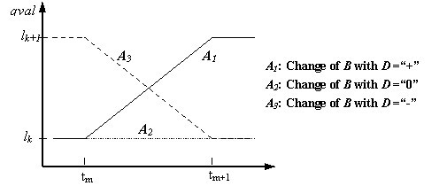
Figure 6. Change of effect variable - 5.7
- For more accuracy, the causality weights among adoption drivers are represented by the path coefficients from the empirical study, indicating the extent to which causal variables influence effect variables. Let the path coefficient represent the causality weight from cost variables on customer utility at time point tm. Let M represent the causality weights from utility variables to cost variables at time point t m+1. According to the feedback effect from utility variables on cost variables, these causality weights are specified as M1= -0.111*∑ qdirxi, M2= 0.493*∑ qdirxi, and M3= 0.256*∑ qdirxi. Thus, the basic causal graph in Figure 4 is extended to the weighted causality in Figure 7.
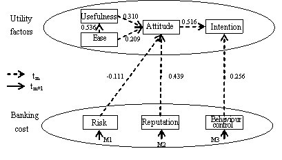
Figure 7. The weighted causality among adoption drivers QSIM Algorithm
- 5.8
- A traditional mathematical approach would not be possible to examine the evolution of causality (or interactions) between determinants with incomplete information. Therefore, QSIM algorithm integrated with weighted causality among adoption drivers in empirical study is used. Since QSIM (Qualitative Simulation) was introduced (Kuipers 1986), it has been commonly used to examine the physical systems (Kuipers 1993a; Kuipers 1993b). There exist many improvements to the QSIM method (Platzner et al 2000; Weld 1990;Shen et al 1993). QSIM enables the exploration on the behavior of physical systems with incomplete information, although it is imperfect. The QSIM method as well as its results, is incomplete (Cem Say and Akyn 2003) and should therefore be utilized in combination with other methods.
- 5.9
- In this paper, we integrated the method with a weighted causal graph (see Figure 4). QSIM consists of four components: qualitative state description, qualitative state constraints, transition rules and a simulation engine (Kuipers 1986). The qualitative state description was investigated above. The weighted causality among adoption drivers in Figure 7 served as a filter to prune the anomalies once the transition yielded successor states.
- 5.10
- As shown in Figure 7, when one cause variable changes, it leads to changes in corresponding effect variables at each time stage. What are these changes? How do effect variables change? The answers to these questions can be obtained using the QSIM algorithm. The transition rules and simulation engine of qualitative simulation are shown as follows.
- The transition rules
The qualitative value of adoption drivers changes only at distinguished time points, including a change of magnitude or change direction. However, the adoption drivers change gradually in the time intervals (Hu and Xia 2005). For example, when the mobile transaction system is upgraded, the banks may provide more safety than they did before the upgrade. Customer perceived risk, however, changes gradually because adopters will take some time to perceive the change of transaction safety.
Rule 1: Parameter setup.
The interaction between cost variables and utility variables has a significant effect on m-banking adoption. Cost variables have an effect on utility variables, and then utility variables have a feedback effect on cost variables.
Rule 2: Reasoning Sequence.
As shown in Figure 7, the reasoning sequence of adoption drivers runs along the arrow direction. However, changes to adoption drivers all occur simultaneously and not along the arrow direction.
Rule 3: Calculation of the change direction in the time intervals: qdir(Z, tm, t m+1).
The adoption drivers change gradually in the time intervals (Hu and Xia 2005). Let qdir(Z, tm, t m+1) be the change direction of adoption driver Zi in the time intervals ( tm, t m+1). According to Figure 7, qdir(Zi, tm, t m+1) depends on the change direction of cause variables Zj at the time point tm. The calculation of qdir(Zi, tm, t m+1) is performed as

(7) in which Zj is the cause variable, Zi is the effect variable, and pji represents the weight of causality from Zj to Zi.
Rule 4: transition of the direction (qdir) and the level (qval) at a time pointtm.
The change of adoption drivers' qualitative value would occur only at distinguished time points. When the accumulation of the causal effect on Zi reaches a certain degree, the level and the direction of Zi will change in the next time stage, or else they remain unchanged. This is an important phenomenon in Customer Relations Management. A manager may achieve a degree of success in promoting m-banking adoption by investment increase. However, if the change degree of the adoption drivers is inadequate, it will be unchanged and not reach a new landmark value.
This phenomenon is expressed as follows: If the change direction of Z in time interval ( tm, t m+1) exceeds 1 or is under -1, the value of Z will change correspondingly and will reach the landmark value L2 (Figure 8(a) and Figure 8(b)). However, if it is between -1 and 1, Z will not change again and will stay at its original values (Figure 8(c) and Figure 8(d)).
.jpg)
.jpg)
(a) Transition of Z with qdir > 1 (b) Transition of Z with qdir < -1 .jpg)
.jpg)
(c) Transition of z with -1 > qdir > 0 (d) Transition of z with 0 > qdir > 1 Figure 8. The transition of state variable z Based on the above regularity, the transition of the direction ( qdir) and the level ( qval) at a time point tm are shown as the following equations:
If qdir(Zi, tm, t m+1) >= 1, then qval(Zi, t m+1)= qval(Zi, tm)+1.
qdir(Zi, t m+1)= qdir(Zi, tm, t m+1)-1.
If -1< qdir(Zi, tm, t m+1) < 1, then qval(Zi, t m+1) = qval(Zi, tm).
qdir(Zi, t m+1) = qdir(Zi, tm, t m+1).
If qdir(Zi, tm, t m+1) <= -1, then qval(Zi, t m+1) = qval(Zi, tm)-1.
qdir(Zi, t m+1) = qdir(Zi, tm, t m+1)+1.Rule 5: State transition.
The change of level and change direction of state variable Z is calculated according to the rules outlined above. The state transitions of Z are illustrated according to the following:
If qval(Zi, tm) = 5 and qdir(Zi, tm, t m+1) = 1, then QS( Zi , t m+1) = (5, qdir(Zi, t m+1)).
If qval(Zi, tm) = 1 and qdir(Zi, tm, t m+1) = -1, then QS( Zi, t m+1) = (1, qdir(Zi, t m+1)).
If 1 < qval(Zi, tm) < 5, then qs(Zi, t m+1) = (qval(Zi, t m+1), qdir(Zi, t m+1)). - Simulation engine
The initial values of utility variables and cost variables are denoted as X0and Y0, respectively. Then the number of feasible solutions (change direction combination of state variables "qdir") is supposed to be N =25. Let n =1, m =0, and the simulation engine is shown as follows:
Step 1: Determine the successor states QS(X, tm) of the utility variable X according to Rule 3 - Rule 5 going along arrow direction in Figure 7. Then let m = m +1.
Step 2: Determine the successor states QS(Y, tm) of the cost variable Y according to Rule 3 - Rule 5 going along arrow direction in Figure 7. Then let m = m +1.
Step 3: If state variables at tm and t m-2 are consistent (i.e., QS(Z, tm) = QS(Z, t m-2)), the variables no longer change over time, and we stop simulation runs. Then, qvaln = QS(Z, tm) is the state value of n-th combination when the adoption behaviour reaches equilibrium. Otherwise, go to Step 1.
Step 4: If n < N, then let n = n+1, and go to Step 1. Or else continue.
Step 5: The neural network is trained using given training data set as shown in Table 3 and Table 4, and the convergent networks are used to represent F and G, which refer to utility function and cost function, respectively.
Step 6: Search optimal solutions by substituting qvaln, qvaln, … , qvaln into the optimisation function as Equation 6 in this paper
- The transition rules
Application and validation of the proposed method
- 6.1
- In this section, we applied the integrated paradigm to solve the optimisation problem in m-banking adoption. The optimal solution influences resource allocation on adoption drivers. A prototype system based on MATLAB 7.0 was built, and its feasibility was validated by comparing the simulation results with real market data and common sense.
Application of the proposed method
- 6.2
- We used Figure 7 as the example. There are many ways by which adoption divers can be changed to improve customer utility and reduce bank costs. We attempted to identify the optimal solution to minimise the marketing costs and maximise the perceived utility.
- 6.3
- For comparison, two opposite scenarios were introduced in which the integrated paradigm was validated. According to a survey by Beijing Unbank Information Consultation Center, there are eight national banks that perform m-banking in China, and their market shares are shown in Table 6. ICBC (Industrial and Commercial Bank of China) with 48,000,000 customers ranked first in domestic m-banking. Conversely, CITIC (China CITIC Bank) was the smallest listed bank, with 72,000 adopters. Therefore, the initial states of ICBC with good market performance and CITIC with bad market performance were summarised as Scenario 1 and Scenario 2, respectively.
Table 6: The number of m-banking adopters in China National Mobile bank Adopter number Data source ICBC (Industrial and Commercial Bank of China) 48,000,000 (ICBC,2011) BOC (Bank of China) 17,000,000 (BOC,2011) CCB (China Construction Bank) 46,950,000 (CCB,2011) BCM (Bank of Communications) 2,000,000 (BCM,2011) CEB (China Everbright Bank) 589,500 (CEB,2011) CIB (Industrial Bank Co., Ltd) 3,720,900 (CIB,2011) CITIC (China CITIC Bank) 72,000 (CITIC,2011) SPDB (Shanghai Pudong Development Bank) 204,800 (SPDB,2011) - 6.4
- The scale items that refer to the initial state of each bank were measured by a ten-point Likert-scale (Beijing Unbank Information Consultation Center 2010). However, the qualitative description method in our model utilised a five-point Likert-scale. Accordingly, the initial state measured by a ten-point scale in Table 7 had to be transformed into qualitative value on a five-point scale in Table 8. Thus, qval0' in Scenario 1 and qval0'' in Scenario 2 refer to the initial state of ICBC and CITIC, respectively.
Table 7: The score for each item on a ten-point Likert-scale Measurement item ICBC BOC CCB BCM CEB CIB CITIC SPD X1 Functional characteristics characteristic 8 9 8 9 7 7 7 8 3G experience 8 8 6 9 6 7 9 4 Browser compatibility 7 8 7 7 8 7 6 8 X2 Activation convenience 7 6 8 8 5 8 4 8 Interface experience 8 7 7 9 5 7 9 6 Operation convenience 8 8 8 9 6 8 8 8 Y1 Safety 9 8 8 8 4 7 4 6 Y2 Customer service 8 5 9 9 8 6 3 6 X3 Usage attitude 10 8 10 6 4 4 10 8 Y3 Preferential policy 8 6 5 8 6 6 2 8 Access speed 8 6 7 8 2 8 4 7 X4 Willingness 8 2 8 2 2 2 8 2 - 6.5
- In simulation runs, two scenarios in the management field were proposed to validate the feasibility of the framework in which the initial level of state variables (qval) was defined (see Table 8).
- 6.6
- Scenario 1: The scenario named as the "good scenario" was abstracted from the initial state of ICBC with good market performance. The initial level combination of state variables qval0 indicates that the level of "perceived usefulness", "perceived usability", "perceived risk", "business credit", "perceived behaviour-control", "using attitude" and "willingness" is high, high, very low, high, very high, high, high, respectively. It is a reasonable portfolio that results in good market performance.
- 6.7
- Scenario 2: The scenario termed as the "bad scenario" represents the initial state of CITIC with poor market performance. The initial level combination of state variables qval0' indicates that the level of "perceived usefulness", "perceived usability", "perceived risk", "business credit", "perceived behaviour - control", "using attitude" and "willingness" is high, moderate, high, low, low, low and very low, respectively. This scenario represents the far-from-optimal investment in each adoption driver that results in the poor market performance.
- 6.8
- In this paper, we examined the optimal resource allocation on adoption drivers to minimise bank costs and maximise customer utility. The simulation results in Scenario 1 and Scenario 2 were qdir' and qdir'', respectively (see Table 8), which can serve as a solution to the optimal problem. In practice, the solution will affect future development priorities and resource allocation on adoption drivers.
- 6.9
- The change direction (qdir) represents change degree, which depends on the investment in adoption drivers. For example, investment in transaction system upgrading will improve perceived safety. The optimal investment proportions in each adoption driver were calculated as follows:

(8) 
(9) Here qdirxi and qdiryj denote optimal change degree and ∑qdirxi+∑qdiryj denote the summation of all of the factors' change degree.
- 6.10
- Denote ip(z) as the optimal investment in "z" with the constraint of marketing budget

(10) in which p(z) denotes the optimal investment proportion in Z and T denotes the total marketing budget.
- 6.11
- For instance, we supposed marketing budget T =1000. Then, the optimal portfolio in Scenario 1 and Scenario 2 was shown as ip' and ip'', respectively. In practice, these optimal portfolios were helpful in maximising customer utility with bank cost constraint.
Table 8: The optimal decision of m-banking investment 0 X1 X2 Y1 Y2 X3 Y3 X4 qval0' 4 4 1 4 5 4 4 dir' 1 0.5 1 -0.5 0.5 1 -0.5 ip' 285.71 285.71 0 142.86 142.86 285.71 142.86 qval0'' 4 3 4 2 2 2 1 dir'' -0.5 1 1 0.5 1 0.5 -1 Ip'' -200 400 400 200 400 200 -400 Validation of the proposed method
- 6.12
- We examined the feasibility of the integrated system framework. Traditionally, two approaches have been used to test validation: basic (quantitative) validation and qualitative validation (Berends and Romme 1999). In this paper, qualitative validation was proposed by comparing simulation outcomes with common sense and real market data.
Comparison of simulation outcomes with common sense
- 6.13
- Applying common sense to simulation outcomes, which allows one to determine simulation results, is reasonable. Psychodynamics denote psychological forces that underlie human behaviour as inner emotional forces and external motivational forces. It is the interaction of these forces that drives the evolution of human behaviour. Human behaviours are regarded as the oscillation between utility gravitation and cost gravitation, then regressing to the equilibrium, which is termed oscillation-equilibrium theory (Neumann 2010).
- 6.14
- In detail, at tm, substitute the optimal solution qdir' and qdir'' into the utility function F and cost function G in Equation 6 to calculate customer utility and bank cost. Denote F(Z)-G(Z)as qualitative values of usage behaviour between utility gravitation and cost gravitation. The adoption process is represented graphically as Figure 9. The results show a transition from oscillation to equilibrium, which is consistent with common sense.
.jpg)
.jpg)
(a) Scenario 1 (b) Scenario 2 Figure 9. The oscillation-equilibrium of interaction among adoption drivers (F-G) Comparison of simulation outcomes with real market data
- 6.15
- To thoroughly validate the integrated paradigm, simulation results were further compared with real market data. A model that can be relied on to reflect the behaviour of the target is valid (Gilbert and Troitzsch 2005). Operational validation is widely utilised to assess how well a decision-making model mirrors real market behaviour (Schutte 2010). Therefore, we performed an operational validation by comparing simulation results with real market data.
- 6.16
- We collected financial data from the two banks, Industry and Commercial Bank of China, Yujiashan Branch; and China CITIC Bank, Yujiashan Branch, which targeted the respondents in the empirical study. Their gross investments in m-banking are 855,000 RMB and 3,200,000 RMB, respectively, and their actual portfolio is shown in Table 9. By substituting the gross investment into Equation 10, the optimal portfolio can be calculated (see Table 9).
Table 9: The simulation outcome and real market data (unit: ten thousands) X1 X2 Y1 Y2 X3 Y3 X4 Scenario 1 Optimal portfolio 91.43 91.43 0 45.71 45.71 91.43 -45.71 Actual portfolio 77.5 60.3 19.2 57.8 30.1 70 12.1 Scenario 2 Optimal portfolio 17.1 34.2 34.2 17.1 34.2 17.1 -34.2 Actual portfolio 18.3 10.4 2.1 27.2 3.5 5.5 18.5 - 6.17
- The actual portfolio and optimal portfolio are shown graphically. Figure 10(a) reveals that the optimal portfolio shows almost the same trend as the actual portfolio in Scenario 1. However, Figure 10(b) reveals obvious differences between the portfolios in Scenario 2, which implies that the actual portfolio is far from optimal. Thus, the integrated paradigm can be further validated by comparing the optimal portfolio with the actual portfolio in two opposite scenarios.
.jpg)
.jpg)
(a) Scenario 1 (b) Scenario 2 Figure 10. Comparison of simulation outcome and real market data (unit: ten thousands)
Conclusions and further work
- 7.1
- This study explores how to minimise bank costs and maximise customer utility in an optimisation model for m-banking adoption. We combined qualitative simulation and empirical study to solve the optimisation problem with incomplete information. Our paper was presented and applied in three components:
- The empirical method was used to examine the interaction among adoption drivers.
- Qualitative simulation was adopted to drive the evolution of adoption drivers.
- The combination of qualitative simulation and empirical study was utilised to solve the optimisation problem with incomplete information.
- 7.2
- A description of interaction among adoption drivers is crucial for an optimisation problem. The ways in which adoption drivers interact refer to the customer utility and the banking costs, which are ambiguous, subjective, incomplete and dynamic. Therefore, these variable correlations cannot be described precisely and completely although a qualitative method may describe the interaction correctly if not exactly. In practice, managers commonly make decisions based on incomplete information rather than precise information. Qualitative information from empirical study is usually adequate. Therefore, we combined the qualitative simulation (QSIM) with the empirical method. This combination has the following advantages:
- QSIM can be used to drive the evolution of interactions among adoption drivers, which account for the complexity of adoption behaviour.
- A basic causal graph in QSIM is too simple and behaves unrealistically without an empirical basis. Empirical study is a valuable enhancement to qualitative simulation.
- 7.3
- Based on the empirical correlations, a qualitative simulation model was built, which included transition rules and a qualitative simulation engine.
- 7.4
- The validation and application above demonstrate that the combination of qualitative simulation and empirical study can serve as a solution to the optimal problem in m-banking adoption, especially with incomplete information. The integrated paradigm provides an effective tool for managers to make decisions that aid in resource allocation to minimise marketing costs and maximise customer utility.
- 7.5
- Further research should seek to improve the following:
- Description of interactions with feedback
The descriptive method seems unavailable for complex interactions with feedback. For further analysis, a more comprehensive causal reasoning method must be developed that will be available for feedback relations.
- Further validation of the integrated method
The validation appropriate for our method is obviously qualitative. Therefore, the validity of the combination needs to be further tested by more cases and experiments.
- Description of interactions with feedback
Appendix
- 8.1
- Build the simulation schedules as follows:
Because in the simulation process, the qualitative simulation and BP neural network is integrated to solve the optimization problem, therefore the loops are separated to several parts.
BP neural network trained as cost function and utility function
load date_input.txt;
load date_output.txt;
p=date_input;
t=date_output;
[R,Q1]=size(p);
[S2,Q2]=size(t);
S1=10;
[w1,b1]=rands(S1,R);
[w2,b2]=rands(S2,S1);
[w3]=rands(Q1,Q2);
p=p*w3;
A1=logsig(w1*p,b1);
A2=purelin(w2*A1,b2);
disp_fqre;
max_epoch;
err_goal;
lr;
TP=[disp_fqre max_epoch err_goal lr];
[w1,b1,w2,b2,epochs,errors]=trainbp(w1,b1,'logsig',w2,b2,'purelin',p,t,TP)
Qualitative simulation
for each combination of change directions
    for t=1:1:100 %t signifies time step or tick
        for each state variable
            % Calculation of the change direction in the time intervals
            for each change direction of other state variables
            dir(i)=dir(i)+dir(j)*p(ji)
            end
            %transition of the direction (qdir) and the level (qval)
            if dir(i)>1
               qval(i)=qval(i)+1
               dir(i)=dir(i)-1
            elseif dir(i)<-1
               qval(i)=qval(i)-1
               dir(i)=dir(i)+1;
            else
               qval(i)=qval(i);
               dir(i)=dir(i);
            end
            %state transition
            if qval(i)>5
               qval(i)=5
            elseif qval(i)<1
               qval(i)=1
            else
               qval(i)=qval(i)
            end
        end
            %test if the variables reach equilibrium
            if qval(t-1)==qval(t)
            break
    end
Calculate the cost and utility
    %cost
    p=qval(X);
    A11 = logsig(w1*p,b1);
    A21 = purelin(w2*A1,b2);
    %utility
    p=qval(Y);
    A12 = logsig(w1*p,b1);
    A22 = purelin(w2*A1,b2);
end
% find out the optimal combination of change directions
[yy,idx]=min(A21) and max(A22);
dir(idx,:);% the optimal change directions
Acknowledgements
- This work has taken place in the Qualitative Simulation Team Work for Complex Management Systems at the Modern Management Institute, Management College, Huazhong University of Science and Technology. It is supported by China National Nature Science Fund (No. 71271093, 71071065) and also in part by the China National Natural Science Fund (Grant No. 71101059; 71101047). The authors would like to thank the anonymous referees for their comments and suggestions on early versions of this paper.
References
-
3G Portal. (2011) "Survey Report on Mobile Banking Adoption in China 2011". http://www.ctiforum.com/news/2011news/04/news0422.htm.
BANK OF CHINA. (2011) "Bank of China 2011 Annual Report". http://www.boc.cn/.
BANK OF COMMUNICATIONS. (2011) "Bank of Communications 2011 Annual Report". http://www.bankcomm.com/BankCommSite/cn/index.html.
BEIJING UNBANK INFORMATION CONSULTATION CENTER. (2010) "War of the mobile banking: A comparison of competitiveness among mobile banks". http://www.docin.com/p-178523726.html#.
BERENDS, R. & Romme, G. (1999), Simulation as a Research Tool in Management Studies. European Management Journal, 17(6):576-583. [doi:10.1016/S0263-2373(99)00048-1]
BERNDSEN, R. (1995). Causal Ordering in Economic Models. Decision Support Systems, 1995, 15:157-165. [doi:10.1016/0167-9236(94)00034-P]
BERNDSEN, R, Daniels H (1994), Causal reasoning and explanation in dynamic economic systems. Journal of Economic Dynamics and Control,18:251-271. [doi:10.1016/0165-1889(94)90078-7]
BRUNER, G. C., & Kumar, A. (2005). "Explaining consumer acceptance of handheld internet devices". Journal of Business Research, 58(5), 553-558. [doi:10.1016/j.jbusres.2003.08.002]
CAMPBELL, D., & Frei, F. (2010). Cost structure, customer profitability, and retention implications of self-service distribution channels: Evidence from customer behavior in an online banking channel. Management Science. 56(1), 4-24. [doi:10.1287/mnsc.1090.1066]
CEM SAY, A. C., & Akyn, H. L. (2003), Sound and complete qualitative simulation is impossible. Artificial Intelligence, 2003, 149: 251-266. [doi:10.1016/S0004-3702(03)00077-8]
CHANG, Y. T. (2002), Dynamics of banking technology adoption: An application to Internet banking. Working paper, University of Warwick, Coventry, UK.
CHASE, R. B. (1978). Where does the customer fit in a service operation? Harvard Business Review, 56(6), 137-142.
CHASE, R. B. (1981). The customer contact approach to services: theoretical bases and practical extensions. Operations research, 29(4), 698-706. [doi:10.1287/opre.29.4.698]
CHATTERJEE, R., & Eliashberg, J. (1990). The innovation diffusion process in a heterogeneous population: A micromodeling approach. Management Science, 36(9), 1057-1079. [doi:10.1287/mnsc.36.9.1057]
CHEN, P. Y., & Hitt, L. M. (2002). Measuring switching costs and the determinants of customer retention in Internet-enabled businesses. Information Systems Research, 13(3), 255-274. [doi:10.1287/isre.13.3.255.78]
CHINA CITIC BANK. (2011) "China CITIC Bank 2011 Annual Report". http://www.ecitic.com/bank.
CHINA CONSTRUCTION BANK. (2011) "China Construction Bank 2011 Annual Report". http://www.ccb.com/cn/home/index.html.
CHINA EVERBRIGHT BANK. (2011) "China Everbright Bank 2011 Annual Report". http://www.cebbank.com/Site/ceb/cn.
CHOI, J., Hui, S., & Bell, D. (2010). Spatiotemporal analysis of imitation behavior across new buyers at an online grocery retailer. Journal of Marketing Research, 47(1), 75-89. [doi:10.1509/jmkr.47.1.75]
DAVIS, D. (1989). Perceived usefulness, perceived ease of use and user acceptance of information technology. MIS Quarterly, 13(3), 318-339.
DAVIS, D., Bagozzi, R. P,, & Warshaw, P. R. (1989). User acceptance of computer technology: A comparison of two theoretical models. Management Science, 35 (8), 982-1003. [doi:10.1287/mnsc.35.8.982]
DOWLING, G. R., & Staelin, R. (1994). A model of perceived risk and intended risk-handling activity. Journal of consumer research, 21(1): 119-134. [doi:10.1086/209386]
GEFEN, D., Karahanna, E., & Straub, D. W. (2003). Trust and TAM in online shopping: an integrated model [J]. MIS Quarterly, 27(1): 51-90.
GERRARD, P., & Cunningham, J. B. (2003). The diffusion of Internet banking among Singapore consumers. International Journal of Bank Marketing, 21(1), 16-28. [doi:10.1108/02652320310457776]
GILBERT, N., & Troitzsch, K. G. (2005). Simulation for the social scientist. (2 edn.; Berkshire, England: Open University Press, McGraw-Hill).
GOOLSBEE, A., & Klenow, P. J. (2002). Evidence On Learning And Network Externalities In The Diffusion Of Home Computers[J]. Journal of Law and Economics, 45(2), 317-343. [doi:10.1086/344399]
GUGLIELMANN, R., & Ironi, L. (2011). A divide-and-conquer strategy for qualitative simulation and fuzzy identification of complex dynamical systems. International Journal of Uncertainty Fuzziness and Knowledge-Based Systems, 19(3), 423-452. [doi:10.1142/S0218488511007076]
HITT, L. M., & Frei, F. X. (2002). Do better customers utilize electronic distribution channels? The case of PC banking. Management Science, 48(6), 732-749. [doi:10.1287/mnsc.48.6.732.188]
HU, B., & Xia, G. C. (2005). Integrated Description and Qualitative Simulation Method for Group Behavior. Journal of Artificial Societies and Social Simulation, 8(2), 1.
INDUSTRIAL AND COMMERCIAL BANK OF CHINA . "Industrial and Commercial Bank of China 2011 Annual Report ". http://www.icbc.com.cn/icbc/.
INDUSTRIAL BANK CO., LTD. (2011) "Industrial Bank Co., Ltd 2011 Annual Report". http://www.cib.com.cn/netbank/cn/index.html.
KAISER, H.F. (1974). An index of factorial simplicity, Psychometrics, 39, 31-36. [doi:10.1007/BF02291575]
KARJALUOTO, H., Mattlia, M., & Pento, T. (2002).Factors underlying attitude formation towards online banking in Finland. International Journal of Bank Marketing, 20(6), 261-272. [doi:10.1108/02652320210446724]
KUIPERS, J. B. (1986). Qualitative Simulation. Artificial Intelligence. 1986,29:289-338. [doi:10.1016/0004-3702(86)90073-1]
KUIPERS, J. B. (1993). Qualitative Simulation: Then and Now. Artificial Intelligence, 1993, 59:133-11 [doi:10.1016/0004-3702(93)90179-F]
KUIPERS, J. B. (1993). Reasoning with qualitative models. Artificial Intelligence, 1993, 59:125-132. [doi:10.1016/0004-3702(93)90178-E]
KOONCE, L., Seybert, N., & Smith, J. (2011). Causal reasoning in financial reporting and voluntary disclosure. Accounting Organizations and Society, 36(4-5), 209-225 [doi:10.1016/j.aos.2011.03.006]
MCFADDEN, L. D. (1974). Conditional logit analysis of qualitative choice behavior. P. Zarembka, ed. Frontiers in Econometrics. Academic Press, New York.
MILIND, S.(1999). Adoption of internet banking by australian consumer:an emperical investigation. International Journal of Bank Marketing,17(7), 324-434. [doi:10.1108/02652329910305689]
NEUMANN, J. E. (2010). How integrating organizational theory with systems psychodynamics can matter in practice: a commentary on critical challenges and dynamics in multiparty collaboration. Journal of Applied Behavioral Science, 46(3), 313-321 [doi:10.1177/0021886310373464]
PLATZNER, M., & Rinner, B. (2000). Toward Embedded Qualitative Simulation: A Specialized
Computer Architecture for QSIM. IEEE Intelligent System, March/April: 62-68.
PURNIMA, S. S., & Preety, A. (2011), Consumer's expectations from mobile CRM services: a banking context". Business Process Management Journal, 17(6), 898-918. [doi:10.1108/14637151111182684]
SCHUTTE, S. (2010). 'Optimization and Falsification in Empirical Agent-Based Models'. Journal of Artificial Societies and Social Simulation, 13 (1), 2. https://www.jasss.org/13/1/2.html.
SHANGHAI PUDONG DEVELOPMENT BANK. (2011) "Shanghai Pudong Development Bank 2011 Annual Report". http://www.spdb.com.cn/chpage/c1/.
SHEN, Q., & Leitch, R. R. (1993). Fuzzy Qualitative Simulation. IEEE Trans. Syst. Man & Cybernet, 1993, 23. [doi:10.1109/21.247887]
STRAUB, D. W.(1989). Validating instruments in MIS research, MIS Quarterly, 13(2): 147-169. [doi:10.2307/248922]
WELD, D. (1990). Exaggeration. Artificial Intelligence, 43: 311-368. [doi:10.1016/0004-3702(90)90077-D]
XUE, M., Hitt, L. M., & Chen, P. Y. (2011). Determinants and outcomes of internet banking adoption. Management Science, 57(2): 291-307. [doi:10.1287/mnsc.1100.1187]