
 Abstract
- Most traditional strategies of assessing the fit between a simulation's set of predictions (outputs) and a set of relevant observations rely either on visual inspection or squared distances among averages. Here we introduce an alternative goodness-of-fit strategy, Ordinal Pattern Analysis (OPA) that will (we argue) be more appropriate for judging the goodness-of-fit of simulations in many situations. OPA is based on matches and mismatches among the ordinal properties of predictions and observations. It does not require predictions or observations to meet the requirements of interval or ratio measurement scales. In addition, OPA provides a means to assess prediction-observation fits case-by-case prior to aggregation, and to map domains of validity of competing simulations. We provide examples to illustrate how OPA can be employed to assess the ordinal fit and domains of validity of simulations of share prices, crime rates, and happiness ratings. We also provide a computer programme for assisting in the calculation of OPA indices.
- Keywords:
- Ordinal, Goodness-Of-Fit, Statistics, Evidence, Validity, Predictions, Observations
Measuring simulation-observation fit:
An introduction to ordinal pattern analysis
- 1.1
- The thrill of programming a computer simulation of social behaviour can seduce its creators to believe that, if it runs, it must be true. Alas a working simulation, however carefully and plausibly constructed, is no guarantee of a valid one, so its creators must sooner or later address a sobering question: How well does the simulation mimic the world it was programmed to simulate? A good fit between a simulation and relevant observations may not be sufficient for establishing the simulation's validity, but it is certainly necessary. In contrast, a bad fit is a simulation's kiss of death—nature's way of telling the programmer to give up or modify the programme and try again. Between good and bad fits is a continuum of so-so, the place where most simulation-observation (S-O) fits in the social sciences are found (see any issue of the Journal of Artificial Societies and Social Simulation).
- 1.2
- The purpose of our present effort is to introduce a simple method of measuring and evaluating simulation-observation fit, and to show how the resulting fitness measures can be used to map domains of validity of competing simulations. We do so by first introducing goodness-of-fit indices, based on matches and mismatches between the ordinal properties of simulation outputs and observations, which we believe have many advantages over traditional approaches to evaluating S-O fit, particularly for the kinds of observations collected in the social sciences. Then we show how to use the indices of S-O fit for detective work needed to explicate conditions under which one simulation is more valid than others.
- 1.3
- Many computer simulations generate outputs representing phenomena that change over time; these are the outputs we shall consider here. Traditional, Euclidean, least-square approaches evaluating S-O fit use measures based on the squared distances between a simulation's outputs and a set of observations (e.g., see Hamilton 1994; Pandit and Wu 1983). In contrast, our approach is based on counts of the frequency of matches between ordered pairs of outputs and ordered pairs of observations. Our approach is congruent with concepts of statistical signatures (Edmonds and Hales 2003; Moss 2001) and stylized facts (Cantner, Ebersberger, Hanusch, Krüger and Pyka 2001; Kaldor 1961).
- 1.4
- The difference between traditional approaches and ours is roughly analogous to the difference between parametric and nonparametric statistics, and between Euclidian geometry and topology. This difference is illustrated in Figure 1, which plots the output of two hypothetical simulations of the selling price of a share of stock in one company across a 13-month period. The output of Simulation A (red line) obviously has a better Euclidean fit to the observed price data (black line) than does the output of Simulation B (blue line); A's output "hugs" the observed prices closely, while B's output wanders from them. In contrast, the output of Simulation B obviously has a better ordinal or topological fit to the price data than does the output of Simulation A; the relative size and shapes of the "wiggles" of B almost perfectly match those of the price data, while A has no wiggles to match.
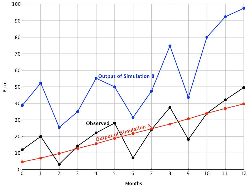
Figure 1. Hypothetical outputs of two simulations of observed stock price data. - 1.5
- Clearly, whether output of simulation A or B should be chosen as having the best fit depends upon the nature of the process being simulated and its purpose. If "hug" is more important than "wiggle," then one should choose A. If the shape of the output and not its average level is important, then one should choose B. There are, of course, occasions when it is sensible to evaluate S-O fit by traditional, Euclidean methods. When a more topological evaluation is desired, it might be sensible to follow the approach outlined below.
- 1.6
- Ultimately, the choice of a method with which to judge simulation fit depends on what is relevant about the particular simulation output and what is thought to be a simulation artefact. It is extremely rare in social simulation that all aspects of the output are important—indicating something real in terms of what is being modelled—usually at least some aspects are attributed to such as "noise." Unfortunately in many reports of simulations, what is and is not considered significant in simulation output is not made explicit. In such cases the choice of method to judge simulation fit is often apparently chosen by default on the basis of tradition (see, for example,Windrum, Fagiolo & Moneta, 2007). If this article prompts simulators to think more carefully about which method is appropriate in their case and make an explicit argument for this in papers, then half its purpose would have been achieved.
Ordinal Pattern Analysis
- 2.1
- Ordinal Pattern Analysis (OPA) is a collection of statistical methods for measuring the extent to which the ordinal properties of a set of predictions match the ordinal properties of a set of observations. Inspired by Denys Parsons' Directory of Musical Tunes and Themes (1975), and developed by Thorngate to assess the fit of longitudinal predictions in psychology (Thorngate 1986a, 1986b, 1992; Thorngate and Carroll 1986), OPA can easily be adapted to evaluate the S-O fit of computer simulations, including simulations with complex outputs.
- 2.2
- The primary OPA index of fit indicates the chances that an ordinal prediction derived from a simulation's output will be matched in the sample of observations at hand. OPA thus addresses the extent to which predictions can be generalized to a sample of observations rather than the extent to which a sample of observations can be generalized to a population. The emphasis on theory-to-sample generalization aligns OPA with Fisher's (1937) principle of randomization, Edwards' (1972) concept of likelihood, and Bayesian statistics (for example, see Lee 2004).
- 2.3
- We believe the principles and practices of OPA are best conveyed by examples, so we begin with an example based on in Figure 1 above. The example shows how to measure the ordinal fit between (1) the outputs of Simulations A and B and (2) the monthly closing share prices of one company. We do this to keep our first example as uncluttered as possible, and to demonstrate that OPA is as useful for evaluating single cases as it is for evaluating hundreds of cases. Later in our article we demonstrate additional uses of OPA when two or more cases are analysed.
- 2.4
- Simulation A. In order to test the fit of the outputs of Simulations A and B to the monthly price of shares in one company, we must first determine the order of all pairs of observations predicted by the output of each simulation. The output of Simulation A predicts that the stock price will go up linearly. As a result, A predicts that, each month (m1 - m12), the share price will be higher than for all preceding months. We express this as a set of predicted ordered pairs, the POP set:
POP (Simulation A) = { m12 > m11, m10, m9, …, m0; m11 > m10, m9, m8, …, m0; … m2 > m1, m0; m1 > m0; m0 > nil }. - 2.5
- There are 13×12/2 = 78 predicted ordinal pairs in the POP set of Simulation A. How many of these 78 orders are matched in the observed price data? We tally them below:
Is m12 > m11? Yes.
Is m12 > m10? Yes.
Is m12 > m9? Yes.
	…
Is m10 > m9? Yes.
Is m10 > m8? No.
…
Is m2 > m1? No.
Is m2 > m0? No.
Is m1 > m0? Yes.
- 2.6
- In sum, 62 of the 78 ordered pairs in the POP set of Simulation A match the corresponding ordered pairs of the share prices. The remaining 78-62 = 16 pairs do not match. So our best estimate of the chances that Simulation A would correctly predict the order of any pair of observations of the stock prices, the probability of a match ( PM), would be:
PM (Simulation A) = #matches / (#matches + #mismatches)
= 62 / (62 +16)
= 62 / 78
= 0.79.
- 2.7
- Restated, PM = 0.79 indicates the output of Simulation A correctly matches 79% of the ordinal relations among the sample of price data of the observed.
- 2.8
- Is PM = 0.79 a good fit? One way to address the question is to consider what we might expect if we had no simulation or other theoretical framework to generate predictions, and relied on flipping a coin to generate them. Predictions of ordinal relations would then be random, and we would expect about 50% of them (PM = 0.50) to be confirmed. Simulation A allows us to increase our predictive accuracy by 58%.
- 2.9
- Researchers inculcated in traditional statistical inference are now likely to ask whether PM = 0.79 is significantly greater than PM = 0.50. To answer the question, we can engage in a touch of mathematical prestidigitation, inventing a derivative index we call the Index of Observed Fit (IOF).
IOF = (2 x PM) - 1. The derivation gives IOF a range from IOF = +1 (all observations match predictions), through IOF = 0 (half the observations match), to IOF = -1 (none of the observations match predictions). In the example above:
IOF (Simulation A) = (2 x 0.79) -1 = +0.58. IOF is a bit like a correlation coefficient. Indeed, when a simulation's output makes predictions about all pairs of observations, and when there are no ties in the observations, then IOF is mathematically equivalent to Kendall's Tau, and its significance level found in relevant Tau tables.
- 2.10
- Simulation B. How do the ordinal predictions of Simulation B's outputs fare? A look at the wiggles of Simulation B in Figure 1 allows us to address the question. Visual inspection of Figure 1 leads to the following predictions.
POP (Simulation B) = { m12 > m11, m10, m9, m8, m7, … m0; m11 > m10, m9, m8, …, m0; m10 > m9, m8, m7, m6, m5, …, m0; m9 > m6, m3, m2, m0; … m4 > m9, m7, m6, m5, m3, m2, m1, m0; m3 > m6, m2; m2 > nil; m1 > m9, m7, m6, m5, m3, m2, m0; m0 > m6, m3, m2 } - 2.11
- Again, there are 13x12/2 = 78 elements in POP set of Simulation B. How many are matched by the price data? As with Simulation A, we now tally.
Is m12 > m11? Yes.
Is m12 > m10? Yes.
…
Is m10 > m9? Yes. Is m10 > m8? No…
Is m9 > m6? Yes. Is m9 > m3? Yes…
Is m4 > m9? Yes. Is m4 > m7? No…
Is m0 > m6? Yes. Is m0 > m3? No. Is m0 > m2? Yes.
- 2.12
- In sum, 72 of the 78 ordered pairs on Simulation B's POP set were matched by the price data, 6 were not. Thus,
PM (Simulation B) = 72 / 78 = 0.92 and
IOF = PM - (1-PM) = 0.84. - 2.13
- The results indicate that Simulation B correctly matches to 92% of the ordinal relations among monthly share prices of the observed stock. Because Simulation B addresses all 78 ordered pairs of the 13 observations, and because there are no ties in the data, IOF is the equivalent of Tau, with a significance level p < 0.01.
Orders of Differences
- 2.14
- Additional ordinal evaluations of S-O fit are also possible. Consider again the plots in Figure 1. Because share prices are measured on a ratio scale, we may subtract prices meaningfully and order their differences. The ordered differences generate a new set of predictions that can be tested with the observed prices.
- 2.15
- Most simulations generate vast numbers of differences between pairs of data in their outputs. For example, each of Simulation B's price outputs for the 13 months shown in Figure 1 can be subtracted from those of the 12 remaining months, creating 12x11 = 132 differences in price, if direction is considered, and 66 price differences if it is not. These 132 (66) can then be compared to 11x10 = 110 remaining differences (55 with direction ignored), generating a possible 14,520 (3,630) distance pairs. Here are two examples:
(m12 - m6) > (m4 - m9)
(m1 - m2) > (m7 - m3) - 2.16
- In principle, all of these orders of differences (POPs) could be used for comparisons with observed results, but not all of them need be. Decisions about whether to consider or ignore the direction of distances, and about which of the often-large set of distance pairs to consider, should be based on their relevance to important features of the simulation under evaluation. The pattern of output of Simulation B (Figure 1), for example, suggests that the simulation exhibits amplified fluctuations: The ups and downs become larger as the months go by. It seems both interesting and important to assess whether the pattern is found in the price data. The first predicted price increase, (m0 to m1) is smaller than the second increase (m2 to m4), which in turn is smaller than the third increase (m6 to m8), which is smaller than the final increase (m9 to m12). Similarly, the first decrease (m1 to m2), is smaller than the second (m4 to m6) which is smaller than the third (m8 to m9). The output thus predicts an additional set of nine ordered pairs:
POP (Simulation B fluctuations) = { (m12 - m9) > (m8 - m6), (m4 - m2), (m1 - m0) (m8 - m6) > (m4 - m2), (m1 - m0) (m4 - m2) > (m1 - m0) (m8 - m9) > (m5 - m6), (m1 - m2) (m5 - m6) > (m1 - m2) } - 2.17
- Eight of these nine predictions are matched in the price data. There is only one mismatch: (m5 - m6) > (m8 - m9). Thus,
PM = 8 / (8+1) = 0.89,
IOF = 2xPM - 1 = 0.78. - 2.18
- As above, our interpretation of PM is straightforward: The POP (Simulation B fluctuations) correctly matched 89% the relevant differences in the observed price fluctuations; as the IOF shows, Simulation B did 78% better than chance. The fit is not perfect, but is respectable. Is it statistically significant? It is not possible to use tables of Tau for estimating a significance level for PM = 0.89 because the POP set does not address all possible distance pairs. We can, however, approximate the p-value by brute force using a simple resampling programme written in "R" (R Core Team, 2012) and shown, with instructions, in the Appendix. Better still, we can try to collect monthly price data for more stocks, then count how many of the stocks each simulation can predict better than chance (PM > 0.50, IOF > 0.00). We will demonstrate how this can be done in a section below.
Congruent and Incongruent Predictions
- 2.19
- Some of the ordinal predictions of Simulations A and B are the same; some are opposite. It is often worthwhile to separate these two sets of predictions to evaluate the predictive accuracy of each. The congruent predictions give us a sense of how well two or more simulations fare when they agree. The incongruent predictions offer the opportunity to pit one simulation against others in a contest of predictive accuracy.
- 2.20
- To illustrate the procedure, consider again the outputs of Simulations A and B. Because Simulation A predicts a monotone increasing trend in the share price, the outputs of Simulations A and B are matched every time they both predict a rise in share price above a precious price. Here is the POP set of these congruent predictions
POP (congruent): { m12 > m11, m10, m9, …, m0 m11 > m10, m9, m8, … m0 m10 > m9, m8, m7, …, m0 m9 > m6, m3, m2, m0 m8 > m7, m6, m5, …, m0 m7 > m6, m3, m2, m0 m6 > m2 m5 > m3, m2, m0 m4 > m3, m2, m1, m0 m3 > m2 m2 > nil m1 > m0 } - 2.21
- There are 59 elements in this congruent set, leaving a set of 78 - 59 = 19 incongruent predictions which are listed below.
POP (B's predictions incongruent with A): { m9 < m8, m7, m5, m4, m1 m7 < m5, m4, m1 m6 < m5, m4, m3, m1, m0 m5 < m4, m1 m3 < m1, m0 m2 < m1, m0 } - 2.22
- How many of the predictions in these two POP sets are matched in the price data shown in Figure 1?
- 2.23
- Matches of congruent predictions = 58; mismatches = 1 (m10 is lower than m8)
PM (congruent prediction) = 58 / (58 + 1) = 0.98 Matches of incongruent predictions (Simulation B) = 15; mismatches = 4
POP (Simulation B, incongruent) = 15 / (15 + 4) = 0.79
POP (Simulation A, incongruent) = 4 / (4 + 15) = 0.21 - 2.24
- In sum, the congruent predictions of Simulations A and B did very well, correctly matching 98% of the ordinal properties of the price data. When the two simulations gave incongruent predictions, Simulation B was clearly superior, correctly matching 79% of the ordinal properties of the price data while Simulation A matched only 21%.
Incomplete Predictions, Missing Data, and Ties
- 2.25
- Simulations A and B make predictions about all 78 pairs of monthly share prices; there are no missing share prices in the data set shown, and none of the share prices are tied. Many simulations, however, do not address every possible pair of observations, and missing data are common, as are ties. Ordinal Pattern Analysis can easily be adapted to these limitations.
- 2.26
- To illustrate how OPA can be employed to handle incomplete predictions, missing data and ties, we turn to a new example. Suppose Simulation C is constructed to generate predictions about violent crime rates in Canada. Varying the variables in Simulation C produces a set of curves with a common shape (a stylized fact): all curves are humped, showing a steady rise in violent crime followed by steady decline. Different settings of the variables produce differences only in when violent crime will peak and in how quickly it will rise or fall (for two examples, see the red and green lines in Figure 2).
- 2.27
- Relevant data on yearly violent crime rates from 1998 to 2010 are available from Statistics Canada (2011). We have modestly modified a few and excluded data from 2007 and 2008 to illustrate how to handle incomplete predictions, missing data and ties. The observed data are also shown in Figure 2.
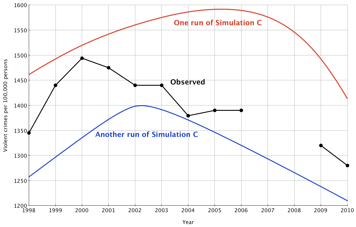
Figure 2. Yearly violent crime rate (CR) in Canada and two runs of Simulation C - 2.28
- Incomplete predictions. In order to test predictions based on the "steady rise, then steady decline" outputs of Simulation C, we need only find the highest observed crime rate, then make predictions about the orders of the rates on each side of the peak but not including the peak. The highest observed crime rate occurred in the year 2000. It is, of course, not kosher to include in our POP set the prediction that all observations on either side of 2000 will be less than the peak; this is true by definition! But we can still make a prediction about the steady rise to the peak by examining the ordinal relations up to and including the observation just before the peak—in this case, 1999:
POP(Simulation C, steady rise) = { CR1998 < CR1999 } - 2.29
- We can also predict that the steady decline from the 2000 peak will be manifested in the following orders from 2001 on. So,
POP(Simulation C, steady decline) = { CR2001 > CR2002, CR2003, CR2004, …, CR2010 CR2002 > CR2003, CR2004, …, CR2010 CR2003 > CR2004, CR2004, …, CR2010 … CR2009 > CR2010 } - 2.30
- Combining the one steady-rise prediction with the 45 steady-decline predictions above gives the complete POP for Simulation C. These 46 predictions fall short of the 78 predictions possible by comparing all pairs of years because no comparisons with the peak in 2000 are allowed, and because no predictions are made between the crime rates for years 1998-1999 versus 2001-2010. Still, we retain 46 predictions for examining matches and mismatches with the observed crimes rates.
- 2.31
- Missing data and ties. How do these 46 predictions fare? None of the predictions involving the years 2007 and 2008 can be tested simply because, as Figure 2 shows, the data are missing. Seventeen of the 46 predictions in POP(Simulation C) are related either to 2007 or 2008 (two examples: CR2005 > CR2007; CR 2008 > CR2010). This leaves us with 29 testable predictions.
- 2.32
- Two of these 29 testable predictions deserve note because the data available to test them are tied: CR2002 = CR2003, and CR2005 = CR2008 (see Figure 2). What should be done with ties when predicting strict greater-than or less-than relations? Four answers are possible: (1) count all ties as matches; (2) count all ties as mismatches; (3) count 50% of the ties as matches and 50% as mismatches; (4) ignore them (seeHollander & Wolfe, 1999). We recommend ignoring them. Excluding ties from the analysis skews the sampling distribution of PM and IOF statistics a bit but, as we shall show below, the skew is unlikely to affect the utility of further analyses.
- 2.33
- If we ignore the two ties, 27 tests of the predictions of Simulation C remain. Of these, only two mismatch the crime rate observations: CR2004 < CR2005 and CR2004 < CR2006; the remaining 25 of 27 predictions match nicely. As a result,
PM = 25 / (25 + 2) = 0.93, and
IOF = 2 x 0.93—1 = 0.86.Simulation C matched 93% of the relevant observations, 86% better than chance.
Analysing multiple data sets
- 2.34
- The examples of one stock's price and one country's crimes above illustrate basic procedures for employing OPA to analyse a single set of longitudinal data. When a researcher is blessed with more than one data set, additional OPA procedures can be invented to analyse them. The additional procedures include the derivation of prototypes, aggregation of results across data sets, and the estimation of domains of validity of two or more simulations.
- 2.35
- In order to illustrate these procedures, consider a new example, this one involving hypothetical data sets of eight people asked to draw a chart of the ups and downs of their happiness across their lifespan. The procedure is simple. Each respondent is given a pencil and sheet of graph paper showing age on the x-axis (birth, 1 year, 2 years, …, 90 years) and happiness on the y-axis (+10 = extremely happy to 0 = extremely unhappy). The respondent then draws a line, usually a wiggly one, plotting from memory how happy he/she was at each year of life. Figure 3 shows plots of the eight participants, A - H, all aged over 70. The solid black line shows their average happiness ratings at 10-year intervals.
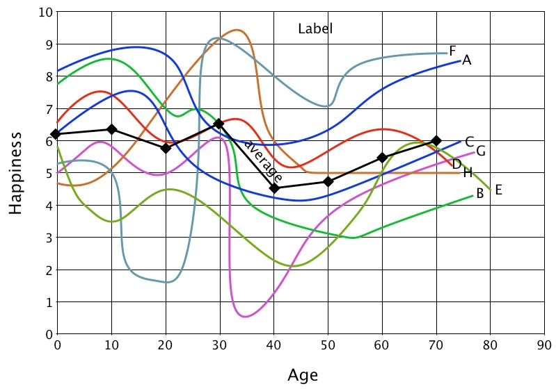
Figure 3. Life-span happiness plots of eight elderly people. - 2.36
- Visual inspection of the eight plots in Figure 3 shows they wiggle all over the map. The plot of the average shows no clear trend beyond a small dip in average happiness around age 40. Still, OPA can sometimes reveal patterns that do not seem apparent by visual inspection or by averaging. These patterns can be used to test the predictive success of various simulations or to guide the development of simulations by revealing what features of their outputs the researcher should examine.
- 2.37
- Prototypes. Did more people increase or decrease their happiness from ages 0 to 10? A look at Figure 3 shows that happiness increased for six participants (A, C, D, E, G, & H) and decreased for two (B and F). Did more people increase or decrease their happiness from ages 0 to 20? Another look at Figure 3 shows that it increased for three participants, decreased for four, and tied for one. Continuing such counts for all 7 + 6 + 5 + 4 + 3 + 2 + 1 = 28 pairs produces a list of the most common ordinal relation ( > or < ) for all of them.
- 2.38
- The result is our definition of a prototype: the POP set producing the highest possible PM across all participants. Table 1 shows the more common ordinal relation, and its PM across the eight participants, for each pair of decades from 0 to 70 shown in Figure 3. The number of participants showing an increase from the row year to the column year are shown to the left of the comma. Those showing a decrease are enumerated to the right of the comma. The red numbers indicate which ordinal relation [Year(X) > Year(Y) versus Year(Y) > Year(X)] accumulated more than half of the participants. Ties (four participants rated X > Y and four rated Y > X) are shown in blue.
Table 1: Number of participants whose happiness ratings went up (left of comma) or down (right of comma) from year to year. To year From year 10 20 30 40 50 60 70 0 6, 2 3, 4 3, 5 2, 6 2, 6 2, 6 4,4 10 2, 6 4, 4 2, 6 1, 7 2, 6 2, 6 20 4, 4 1, 7 1, 7 3, 5 3, 5 30 0, 8 1, 7 3, 5 3, 5 40 5, 3 6, 2 7, 1 50 7, 0 6, 1 60 6, 1 - 2.39
- From the counts in Table 1 we can construct the elements of the prototype POP set using "majority rule": The more common ordinal relation prevails. The three pairs showing ties, (Y0, Y70), (Y10, Y30, and (Y29, Y30), are excluded from the prototype.
POP(prototype) = { Y0 < y10, y0 > Y20, Y0 > Y30, Y0 > Y40, Y0 > Y50, Y0 > Y60, Y10 > Y20, Y10 > Y40, Y10 > Y50, Y10 > Y60, Y10 > Y70, Y20 > Y40, Y20 > Y50, Y20 > Y60, Y20 > Y70, Y30 > Y40, Y30 > Y50, Y30 > Y60, Y30 > Y70, Y40 < y50, y40 < y60, y40 < y70, y50 < y60, y50 < y70, y60 < y70 } - 2.40
- Figure 4 shows two plots that meet the ordinal constraints of POP(prototype) above. The average happiness rating across the eight participants is also shown for comparison. Units of happiness are omitted in the Y-axis to indicate that the three plots show only relative (ordinal) relations among their nine points; only their shapes are relevant. Note that the two plots of the prototype show peak happiness at age 10. In contrast, the average happiness peaks at 30. It is another illustration that what is true in general is not always true on average.
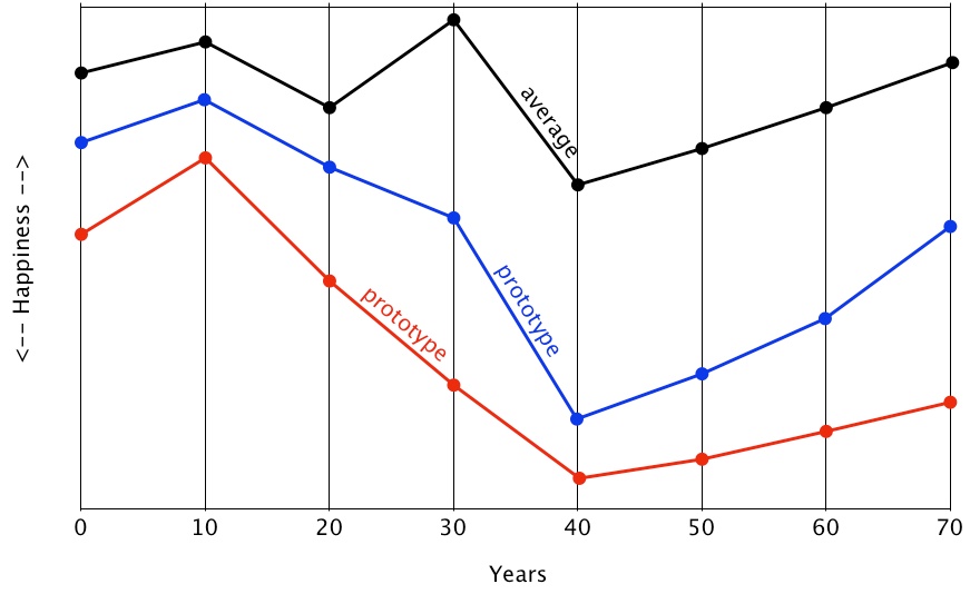
Figure 4. Two prototypes with the ordinal constraints of most participants. - 2.41
- The prototype gives us the POP set that will maximize the likelihood of predicting the ordinal relation of any randomly chosen pair of happiness ratings from any of the eight participants. It is, in short, the best any POP set can do, including any POP set generated by a simulation.
- 2.42
- How good is best? To address the question, it is useful to determine how well the prototype fits the ordinal pattern of each of the eight participants' happiness ratings. Excluding from comparison the three "<>" relations among the 28 elements in POP(prototype) set, we count how many of the remaining 25 elements match the happiness ratings of persons A - H shown in Figure 3. The results are shown in Table 2.
Table 2: Ordinal fit of individual happiness plots to prototype Participant A B C D E F G H Total Matches 21 23 22 23 19 11 21 12 152 Mismatches 4 2 3 2 6 14 3 10 44 PM = 0.84 0.92 0.88 0.92 0.76 0.44 0.88 0.54 0.78 IOF = +0.68 +0.84 +0.76 +0.84 +0.52 -0.12 +0.76 +0.08 +0.56 - 2.43
- Table 2 reveals that the prototype did a moderate-to-good job of matching the ordinal patterns, reproducing on average 78% of the ordinal relations among each participants happiness ratings. There were, however, notable individual differences. The prototype matched the ordinal patterns of participants A, B, C, D, E and G quite well. However, it did not reproduce the ordinal patterns of F and H well; it did little better than chance matching the pattern of H, and worse than chance matching the pattern of F.
- 2.44
- Like a string of averages (see Figure 4), the prototype provides a standard for comparing how well the output of one or more simulations matches a set of observations such as the set shown in Figure 3. A simulation generating an ordinal pattern far different from the prototype is likely to have little validity. When the ordinal pattern of the prototype diverges from that of the averages, a researcher must choose a preferred standard of comparison. We vote for the prototype, simply because it is less sensitive than are averages to violations of assumptions about normality, scale, and independence of observations that make averages useful. When a researcher wishes to address how well a simulation matches observations in general rather than on average — counting instances rather than measuring distances — prototypes should be preferred.
- 2.45
- Our definition of a prototype is not the only one that might be useful for analysing prediction-observation fit. The definition we employ constrains ordinal patterns to fixed time periods—to each decade in the example above. It is possible that the "up-down" wiggles of one person match those of others but occur at a slower or faster rate. To explore this possibility, OPA can be extended to examine the ordinal patterns of peaks and valleys, zeniths and nadirs, comparing their relative heights across time without reference to a fixed time interval. A researcher need only identify the data points at which an up or down trend changes direction, make predictions based on simulation outputs about the order of heights of these directional changes, and calculate PM from number of matches to the data at hand.
Combining Results Across Studies
- 2.46
- As noted in in the beginning of this article, Ordinal Pattern Analysis was designed to address how well the predictions of a theory, or the equivalent outputs of a simulation, match a sample of observations. OPA was not designed to address how well a sample of observations can generalize to a population. Still, it is reasonable to assume that our degree of belief in the generality of a simulation based on hundreds of large samples from diverse populations would be higher than our degree of belief based on one small sample. The assumption drives interest in meta-analysis as a collection of methods for combining research results across studies (see, for example, Hedges and Olkin 1985).
- 2.47
- OPA can easily be adapted to capture the spirit of meta-analysis. Fortunately, the creators of computer simulations must be quite explicit about their creations' assumptions because the assumptions must be translated into lines of programming code. As long as a set of observations meets these explicit assumptions, the set is fair scientific game for testing the simulation. So if Study S1 matches 16 out of 20 predictions of theory T (PM = 0.80), and if Study S2 matches 122 out 173 predictions of theory T (PM = 0.70, then across these studies, theory T has matched 16+122 out of 20+173 predictions (PM = 0.71). To assist in combining in this way across several studies, it is thus advisable for the authors of each study to report their raw numbers of matches, mismatches, and ties.
Explicating Domains of Validity
- 2.48
- Best-fitting models and prototypes rarely capture all the ordinal patterns of all observations. As illustrated by the data from Persons H and F in the prototypical example above, noticeable deviations—outliers—are almost certain to occur. When these deviations are rare, it is tempting to ascribe them to sampling error and focus on generalities. But the more frequently the deviations occur, the more prudent it becomes to suspect that different processes are generating them, each process captured by a simulation with different assumptions (see, for example, Bonini 1963; Levins 1966; Thorngate 1975, 1976).
- 2.49
- The history of social science tells us that few, if any, assumptions about human activity are entirely invalid across all people, situations and time; in fact, the opposite far more persistent. As social science data accumulate, almost all statements about what people do "in general" are modified by an ever-expanding list of conditionals and context dependencies, by a litany of "it depends" (Thorngate 1976). There are, for example, hundreds of ways for people to make decisions: do what they have done before, do what they have not done before, do what others are doing now, ask for advice, compare lists of pros and cons, consider the chances of costs and benefits, pray, consult statutes, flip a coin, etc. All of these are used by some people in some situations at some time (and not others), and many of them lead to different outcomes in real life as well as in simulations.
- 2.50
- There is increasing evidence that human cognition is "wired" to be context-dependent—different people do have coherent and consistent behaviours but they will be differentially invoked in different kinds of circumstances (Edmonds 2012). Exactly how human cognition does this is unclear. However it seems to be done in an information rich and largely unconscious manner, allowing for reliable co-recognition of different kinds of situations but making their reification in terms of precise boundaries hard (Edmonds 1999, 2012).
- 2.51
- It therefore seems misguided to pit simulations against on another in a general contest of greatest validity across people, situations and time. Instead, it seems more prudent to assume that each simulation will be valid for different combinations of people, situations and time. With this assumption, it is then sensible to explicate the conditions under which each simulation is more valid than others—thus mapping its domain of validity (Thorngate 1975, 1976). It is also sensible to assume that the boundaries separating domains of validity will not be immutable or precise. The domains are likely to be represented best as statistical equivalents of fuzzy sets, with degrees of membership based on frequency, rather than arbitrary cutoffs—degrees similar to fuzzy sets of "tall people" or "cloudy days" (Zadeh 1965) and detected by neural network, cluster analysis or related techniques.
- 2.52
- Several techniques now exist to assist in mapping the domains of validity of different models and simulations, among them cluster analysis (for example, see Aldenderfer & Blashfield 1984) and discriminant function analysis (see Klecka 1980). Ordinal Pattern Analysis can be adapted to accomplish the task as well. We shall illustrate this adaptation in a future manuscript.
Discussion
- 3.1
- Our introduction to Ordinal Pattern Analysis has offered a brief overview of its assumptions and methods. Space prohibits us from providing more variations and examples, or from wading into the deep philosophical waters of model verification (Windrum, Fagiolo and Moneta 2007). Excluded from our presentation are techniques for measuring the relevant closeness of fit of all kinds of simulation output. For example, if a certain ordinal pattern was being predicted but not when it would occur, the above techniques would have to be expanded to in manners similar to those of elastic matching (Uchida 2008) and dynamic time warping (see Myers and Rabiner 1981). What is important is that the relevant aspects of the simulation output are compared in an appropriate way to the data. There are no doubt dozens of special cases requiring further refinements of OPA. We hope others will develop and publish them.
- 3.2
- It is important to remember that a good simulation-observation fit is necessary for validating a simulation's outputs, but it is not sufficient. Other simulations based on alternative assumptions (often called possible confounds) might generate outputs that fit the observations at least as well. Experimental designs, statistical procedures, and analyses of special cases often hold some promise of separating the validity of a simulation from the validity of its possible confounds. But, to paraphrase Coombs (1964), we buy the discriminating power of these techniques with the currency of their assumptions. One of their assumptions is that either a simulation or one of its possible confounds is valid, but not both. In the world of social simulation it is probably safer to assume that all assumptions are valid for at least one instance. As a result, the task of validation becomes the task of mapping the size and shape of valid domains.
- 3.3
- Faced with this task, it becomes equally important to understand that a simulation showing a bad fit to some collections of data might still show a good fit to others, including others collected in the future. This is especially true when simulating socio-cultural process based on acquired psychological processes. Consider, for example, the cognitive processes that generate evening meals. Almost all of these processes are learned, some by trial-and-error, most by a social communication process coded in an artefact called a recipe. There are thousands of extant recipes; hundreds more are added each day. Their popularity rises with fashion and falls with boredom. So any simulation predicting the proportion of people eating, say, poached salmon with a maple-walnut glaze might show a bad fit in Mexico but good S-O fit among small-town Canadians for 18 months following the publication of a popular salmon recipe book. There is, in short, little reason to reject any simulation based on a bad S-O fit to one data collection. There is instead good reason to report the conditions under which a bad fit was obtained.
- 3.4
- The task of comparing the S-O fit of competing simulations is relatively easy for simulations with few variables, but becomes much more complex as the number of variables increases, leading to what is sometimes called the parameter identification or free parameter problem (Greeno and Steiner 1964; Koopmans 1949). Simulations with dozens or hundreds of variables have a pernicious tendency to generate a wide variety of conceivable outputs, often enough to account for all possible observations. Evaluating their validity then becomes less a matter of finding good fits and more a matter of validating the settings of variables that generate these good fits. Addressing this matter would require, in turn, that the unit of analysis for assessing domains of validity shift from the observed behaviour to the process or algorithm generating the observed behaviour (Thorngate 1975, 1976). If OPA could help infer the conditions that influence the popularity of different psychological processes generating the observations researchers analyse, it would serve a useful function.
Appendix
- 4.1
- The computer programme below was written as a simple, calculator-style aid for tallying matches, mismatches and ties, for computing PM and IOF indices, and for estimating the probability that random permutations of data might have produced values of PM and IOF at least as big as those obtained. It does not do fancy statistical analyses, but does save you time counting matches, mismatches and such for a data set produced by one person/group/situation over time. We hope that others will add more features and sophistication to the programme.
- 4.2
- In order to install and run the programme (written in the programming language "R"; see R Core Team 2012) on your computer, here is what to do:
- Download the programming language "R" from http://www.r-project.org
- Install R on your computer
- start R and select from its menu the "Create a new, empty document in the editor" icon (the one to the left of the printer icon at the top of the R window in version 2.14);
- copy the entire programme listed below;
- paste it into the R editor;
- save the programme on your hard disk or other safe place under the name "OPA";
- load this OPA file into R using the "Source file" command under the "file" menu
- 4.3
- You are now ready to input some predictions and observations for the OPA programme. Here is an example of how to do it. Suppose you have a simulation showing that people accumulate friends as time goes by. The simulation thus predicts that for any two years, someone will report more friends in the later year than in the former year. We conduct a small study asking Mary, aged 12, to list her friends each year age 12 to age 17, and asking John, aged 56, to do the same for each year from age 56 to 61.
- 4.4
- Suppose Mary reports the following numbers of friends for the years 12-17:
5, 3, 8, 11, 10, 11. - 4.5
- Suppose John reports the following numbers of friends for years 56-61, but forgets to do it in his 60th year, leading us to enter "NA" (not available) as a placeholder:
29, 24, 26, 19, NA, 20. - 4.6
- We enter Mary's data into the computer programme this way:
mary = c(5,3,8,11,10,11)
then we enter John's data this way:
john = c(29,24,26,19,NA,20)
[note: the lower-case "c" in each line means "catenate" or string together- a quirk of the R language] - 4.7
- Now we enter the predictions of our simulation. We label the youngest year "Year 1" or 1 for short. We label the next year "Year 2" or 2 for short. Then we enter the predictions, the POP set, into the computer programme in this way:
predictions = c(6,5,6,4,6,3,6,2,6,1,5,4,5,3,5,2,5,1,4,3,4,2,4,1,3,2,3,1,2,1)
The first two numbers in this list (6,5) mean, "In the 6 th year of the study (when Mary is 17 and John is 61) Mary and John will report more friends than in the 5th year of the study (when Mary is 16 and John is 60)." The next two numbers in this list (6,4) mean, "In the 6 th year of the study (when Mary is 17 and John is 61) Mary and John will report more friends than in the 4th year of the study (when Mary is 15 and John is 59)." - 4.8
- The pairs of numbers in the "predictions" POP set continue this way until the final pair: 2,1 meaning "In the 2nd year of the study (when Mary is 13 and John is 57) Mary and John will have more friends than in the 1st year of the study (when Mary is 12 and John is 56)."
- 4.9
- Once the three containers of numbers (AKA variables): mary, john and predictions are entered, we can then run the OPA programme. Shown in boldface is what to type to run the programme to test how well Mary's reports match the predictions of the simulation:
calcopa(predictions, mary) and here is the output of the programme: matches mismatches ties NAs 12 2 1 0 [1] PM (probability of a match = 0.857 [1] IOF (index of observed fit) = 0.714 [1] Prob of matches >= obtained matches = 0.043 - 4.10
- Here is what to type to run the programme for John's reports:
calcopa(predictions, john) and here is the output of the programme: matches mismatches ties NAs 2 8 0 5 [1] PM (probability of a match = 0.200 [1] IOF (index of observed fit) = -0.600 [1] Prob of matches >= obtained matches = 0.943 - 4.11
- The output also includes a "p-level" for the significance of the obtained PM and IOF for those who wish to use it. The p-level is calculated using standard resampling procedures (see, for example, Good, 2005).
- 4.12
- Below is the Ordinal Pattern Analysis (OPA) programme.
calcopa=function(pred,obs) {
	realmatches=calcmatches(pred,obs) ## get hits for real data
	print(realmatches)
	PM=realmatches[1]/sum(realmatches[1:2])
	## options(digits = 4, width = 80)
	x=formatC(PM, digits=3, format="f")
	print(c("PM (probability of a match) =",toString(x)),quote = FALSE,digits = 4)
	IOF=2*PM-1
	x=formatC(IOF, digits=3, format="f")
	print(c("IOF (index of observed fit) =",toString(x)), quote = FALSE)
	## now shuffle data 1,000 times to see how often #hits is > realmatches
	nobs=length(obs)
	exceeds=0 ## set exceeds counter to zero
	for(j in 1:1000) {
		obs=sample(obs,nobs)
		randmatches=calcmatches(pred,obs)
		if(randmatches[1]>=realmatches[1]) {
			exceeds=exceeds+1
		}
	}
	print(c("Prob of matches >= obtained matches =",toString(exceeds/1000)), quote = FALSE)
}

calcmatches=function(pred, obs) {
## function to compute ordinal pattern hits, misses, and ties
first=pred[seq(1,length(pred),2)]
second=pred[seq(2,length(pred),2)]
hits = sum(obs[first] > obs[second], na.rm=TRUE)
ties = sum(obs[first] == obs[second], na.rm=TRUE)
misses = sum(obs[first] < obs[second], na.rm=TRUE)
NAs = sum(is.na(obs[first] > obs[second]))
return(unlist(data.frame(hits, misses, ties, NAs)))
}
Acknowledgements
- The authors wish to thank two anonymous reviewers for their helpful comments on a previous draft of this manuscript, and for suggestions to improve the computer programme in our Appendix. Bruce Edmonds was supported by the Engineering and Physical Sciences Research Council, grant number EP/H02171X/1.
References
- ALDENDERFER, M. and Blashfield, R. (1984). Cluster analysis. Beverley Hills, CA: Sage Publications.
BONINI, C. (1963). Simulation of information and decision systems in the firm. Englewood Cliffs, NJ: Prentice-Hall Inc.
CANTNER, U., Ebersberger, B., Hanusch, H., Krüger, J.J. and Pyka, A. (2001). Empirically Based Simulation: The Case of Twin Peaks in National Income. Journal of Artificial Societies and Social Simulation 4(3):9 http://www.soc.surrey.ac.uk/JASSS/4/3/9.html
COOMBS, C. (1964). A theory of data. Oxford: Wiley & Sons.
EDMONDS, B. (1999). The Pragmatic Roots of Context. CONTEXT'99, Trento, Italy, September 1999. Lecture Notes in Artificial Intelligence, 1688, 119-132. [doi:10.1007/3-540-48315-2_10]
EDMONDS, B. (2012). Context in Social Simulation—why it can't be wished away. Computational and Mathematical Organization Theory, 18(1), 5-21. [doi:10.1007/s10588-011-9100-z]
EDMONDS, B. and Hales, D. (2003). Replication, Replication and Replication: Some Hard Lessons from Model Alignment. Journal of Artificial Societies and Social Simulation, 6(4):11 https://www.jasss.org/6/4/11.html
EDWARDS, A.W.F. (1972). Likelihood. Cambridge: Cambridge University Press.
FISHER, R. (1937). Statistical methods and scientific inference. New York: Hafner Press.
GOOD, P. (2005). Permutation, parametric, and bootstrap tests of hypotheses (3rd Edition). New York: Springer-Science + Business Media, Inc.
GREENO, J. and Steiner, T. (1964). Markovian processes with identifiable states: General considerations and applications to all-or-none learning. Psychometrika, 29(4), 309-333. [doi:10.1007/BF02289599]
HAMILTON, J. (1994). Time Series Analysis. Princeton: Princeton University Press.
HEDGES, L. and Olkin, I. (1985). Statistical methods for meta-analysis. Orlando, FL: Academic Press, Inc.
HOLLANDER, M. and Wolfe D. (1999). Non-parametric Statistical Methods (2nd edition). New York: Wiley & Sons, Inc.
KALDOR, N. (1961). Capital accumulation and economic growth. In F.A. Lutz & D.C. Hague (Eds.), The Theory of Capital. London: St.Martins Press, 177–222.
KLECKA, W. (1980). Discriminant analysis. Quantitative Applications in the Social Sciences Series, No. 19. Thousand Oaks, CA: Sage Publications.
KOOPMANS, T. (1949). Identification problems in economic model construction. Econometrica, 17(2): 125-144. [doi:10.2307/1905689]
LEE, P. (2004). Bayesian statistics: An introduction (3rd Edition). London: John Wiley & Sons, Ltd.
LEVINS, R. (1966). The strategy of model building in population biology. American Scientist, 54, 421-431.
MOSS, S. (2001). Game Theory: Limitations and an Alternative. Journal of Artificial Societies and Social Simulation, 4(2):2 http://www.soc.surrey.ac.uk/JASSS/4/2/2.html [doi:10.2139/ssrn.262547]
MYERS, C. and Rabiner, L. (1981)._ A comparative study of several dynamic time-warping algorithms for connected word recognition._ The Bell System Technical Journal, 60(7): 1389-1409. [doi:10.1002/j.1538-7305.1981.tb00272.x]
PANDIT, S. and Wu, S-M. (1983). Time Series and Systems Analysis with Applications. New York: John Wiley and Sons.
R CORE TEAM (2012). R: A Language and Environment for Statistical Computing. Vienna, AT: R Foundation for Statistical Computing, http://www.R-project.org/
STATISTICS CANADA (2011). Incident-based crime statistics, by detailed violations, annual (CANSIM Table 252-0051). Ottawa: Statistics Canada. Available at http://www4.hrsdc.gc.ca/.3ndic.1t.4r@-eng.jsp?iid=57
THORNGATE, W. (1975). Process invariance: Another red herring. Personality and Social Psychology Bulletin, 1, 485-488. [doi:10.1177/014616727500100304]
THORNGATE, W. (1976). In general vs. it depends: Some comments on the Gergen-Schlenker debate. Personality and Social Psychology Bulletin, 2, 404-410. [doi:10.1177/014616727600200413]
THORNGATE, W. (1986a). The production, detection, and explanation of behavioural patterns. In J. Valsiner (Ed.), The individual subject and scientific psychology. New York, Plenum, pp. 71-93. [doi:10.1007/978-1-4899-2239-7_4]
THORNGATE, W. (1986b). Ordinal pattern analysis. In W. Baker, M. Hyland, H. van Rappard, & A. Staats (eds.), Current issues in theoretical psychology. Amsterdam: North Holland, pp. 345-364. [doi:10.1007/978-1-4899-2239-7_9]
THORNGATE, W. (1992). Evidential statistics and the analysis of developmental patterns. In J. Asendorpf & J. Valsiner (Eds.), Stability and change in development: A study of methodological reasoning. Newbury Park, CA: Sage, pp. 63-83.
THORNGATE, W. and Carroll, B. (1986). Ordinal pattern analysis: A method for testing hypotheses about individuals. In J. Valsiner (Ed.), The individual subject and scientific psychology. New York, Plenum, pp. 201-232. [doi:10.1007/978-1-4899-2239-7_9]
UCHIDA, S. (2008). Elastic matching techniques for handwritten character recognition. In B. Verma, & M. Blumenstein (Eds.), Pattern Recognition Technologies and Applications: Recent Advances (pp. 17-38). Hershey, PA: Information Science Reference. [doi:10.4018/978-1-59904-807-9.ch002]
WINDRUM, P., Fagiolo, G. and Moneta, A. (2007). Empirical validation of agent-based models: Alternatives and prospects. Journal of Artificial Societies and Social Simulation, 10(2),8 https://www.jasss.org/10/2/8.html
ZADEH, L (1965). Fuzzy sets. Information and Control, 8, 338-353. [doi:10.1016/S0019-9958(65)90241-X]