
 Abstract
- In recent decades, compact cities have become a new concern in urban planning in most Japanese cities. The main reason for this trend among Japanese cities is the phenomenon of de-urbanization and downtown decline that gradually occurred after the 1990s. As such, at present, there are dispersed, small, built-up portions of suburban areas that have resulted in household mobility outside the downtown. Therefore, some local governments in Japan are attempting to realize compact cities through policy intervention, such as encouraging households to relocate from suburban to downtown areas in order to address the population decline in urban areas. Recently, one such residential policy have been promoted by Japanese local city governments. By offering a local housing allowance, this policy encourages households to relocate to downtown areas. We developed an agent-based household residential relocation model (HRRM) to visualize the effect of this residential policy, that is, the local housing allowance. The HRRM is built on householdsÄô adaptive behaviours and interactions through housing relocation choices and policy attitudes, and so it can simulate the diversified residential relocations of households in various lifecycle stages. Through simulation using the HRRM, the effectiveness of this residential policy can be visualized, and the HRRM will help local governments to understand the effects of residential policies.
- Keywords:
- Household Relocation, Downtown Decline, Compact City, Urban Shrinkage, Policy Effect
Introduction
- 1.1
- For a number of decades, urban issues related to housing markets and residential mobility were concerned primarily with such topics as urbanization and sprawling settlements (Haase et al. 2010; Antrop 2004; Kazepov 2005). Now, however, urban shrinkage is a hot topic among urban planners (Rieniets 2005; Rieniets 2009). As the population density decreases, households in a lower-density, built-up city require more private vehicles (Kaido 2005). This trend appears not to follow that desired by urban planners — namely, to reduce the negative environmental impacts associated with car dependency (Newman and Kenworthy 1989; Banister 1997; Banister et al. 1997). Thus, methods for revitalizing downtown areas are being considered by many governments and urban planners. In most Western societies today, policy prescription has increasingly favoured a compact city approach in order to address the adverse effects of urban shrinkage (Howley et al. 2009). In this paper, we will introduce the household residential relocation model (HRRM), which is an agent-based model (ABM) for simulating the household residential relocation process effected by a residence promotion policy. The HRRM integrates the adaptive behaviours of households in terms of residential relocations with policy interactions to visualize the impact of a residence promotion policy on downtown revitalization.
- 1.2
- Residential relocation actually is not a new topic; much research already exists in this field. From a broader perspective, researchers generally attempt to address their concern about residential location issues by analyzing the relationship between household residential location choice and transportation. Stated preference experiments in this field focus primarily on determining the relationship between transport characteristics and residential location (Kim et al. 2005; Molin and Timmermans 2003; Rouwendal and Meijer 2001). These studies are based primarily on statistics instead of on agent-based simulations. In addition, researchers also have investigated interactive processes between transportation and land use in order to model the distribution of populations across space. As an example, Land Use Transport Interaction (LUTI) was first developed as an aggregated model (Timmermans 2003), describing the allocation of population as an aggregate category. Gradually, LUTI models were improved to agent-based (Benenson 1998; Miller et al. 2004; Waddell et al. 2003; Ettema et al. 2006; Moeckel et al. 2005), which can describe the location behaviour of individual households. Another representative model is UrbanSim (Noth et al. 2003), which adopts a micro simulation approach in which it represents individual agents within the simulation. In UrbanSim, a household mobility model is presented to simulate the relocation of a household closer to employment, which is an evolutionary process resulting from interactions between different urban actors, land use, and transportation. Thus, LUTI and UrbanSim are similar in that they are both integrated frameworks for simulating the interactive process of land use, transportation, and residential choice. They show a strong ability to simulate the spatial process but their focus on the interactions of adjacent agents is relatively weak.
- 1.3
- Because this research simulates household behaviour during residential relocation with respect to a residence promotion policy, however, the model here needs a strong capacity to reflect agents' policy interactions. Thus, an agent-based approach is more suitable than micro simulations. As reported previously (Jager 2007), an ABM is expected to contribute to exploring the effectiveness of policy measures in complex environments through behaviour-environment interactions. A number of studies have used an ABM to assess future the socio-ecological consequences resulting from land-use policies (Lee et al. 2010), and other studies have focused on the use of multi-agent simulation for policy development (Berger et al. 2006). As an agent-based simulation, the residence promotion policy will be taken as a key for organizing agent interactions in the HRRM. Unlike micro-simulation, the HRRM emphasizes interaction between households during the decision processes of household agents with respect to residential location. During such a time, household agents evolve stochastically to adapt themselves to urban space in response to the changes of lifecycle stages and the residence promotion policy, whereas traditional micro simulation transition probabilities lack evolutionary and spatial dimensions. The decision process of household residential location can be simplified into two phases: the evaluation of the current residence and the selection of a new one (Boyle et al. 1998). A household residential location change, as defined by previous studies, can be classified as either an induced relocation or as an adjustment relocation (Cadwaller 1992; Clark and Onaka 1983). An induced relocation is linked to changes in an individual's lifecycle stage (Kulu and Milewski 2007; Mulder and Wagner 1998). This means that individuals who enter a new lifecycle stage are the most likely to relocate (Kulu 2007). On the other hand, adjustment relocation is related to dissatisfaction with the current location (Kährik et al. 2012), with the decision to relocate depending on the satisfaction of the residents with their current location. When the satisfaction with current housing is below a certain threshold, individuals will start to search for an alternative place of residence. Both induced and adjustment relocations are included in the HRRM as adaptive behaviours in the residential relocation process.
- 1.4
- ABMs are widely used for residential simulation from the viewpoint of economics with respect to real estate, in which housing prices are an important factor. Based on the assumption that gentrification occurs because capital flows back to the inner city and creates opportunities for residential relocation, Diappi and Bolchi (2006) presented a dynamic model developed on a Netlogo platform and using a multi-agent/cellular automata system approach. By describing the relocations of households, researchers have, to some extent, addressed the housing market processes and price formation (Ettema 2011; Dawn 2008). In particular, Moeckel simulated the process by which households evaluate individual dwellings until they eventually find and accept a dwelling that offers a significant improvement over their current dwelling (Moeckel et al. 2003). This is similar to the proposed HRRM, where utility is used by households to evaluate different locations. However, unlike in the study by Moeckel, in the proposed HRRM, utility comparison is only one step of the entire relocation process for adapting households to the urban environment. Furthermore, the present study does not focus on the urban sprawl process of residential location choices. Rather, we focus on how to simulate household residential relocation choices as influenced by a local residence promotion policy; we further consider how that policy influences household residential relocation and consequently downtown revitalization during urban decline.
- 1.5
- With respect to our contribution, this model can simulate the process of household residential relocation influenced by a residence promotion policy for downtown revitalization. Unlike conventional simulations of residential relocation, the HRRM not only can simulate households' adaptive behaviours of residential relocations in a predefined urban space but also can reflect the influences of policy implementation on households' relocation process through organizing policy interactions among household agents. The simulation result can be visualized, and households that have relocated to downtown areas can then be identified. In the following section, we describe how the HRRM is constructed and used. The remainder of this paper is organized as follows: the HRRM will be described in detail in section 2. Section 3 illustrates the initial conditions and simulation configuration for using HRRM. Section 4 is a test of model sensitivity on changes owing to both household lifecycle stages and policy effects, and is also a comparison between simulated results and the real city data of a typical Japanese city. Finally, the research results are discussed and conclusions presented in section 5.
Model Formulation
-
Structure of the HRRM
- 2.1
- Regarding the incentives of residential locations, some existing research has proposed that the changes in household lifecycle stages lead to relocation behaviour (Fontaine and Rounsevell 2009; Torrens 2001). This conclusion is not absolute because 'induced' and 'adjustment' moves play different roles. In the HRRM, we assume that when the lifecycle stage changes, a household agent may express interest in relocation, although the final decision as to whether to relocate depends on the household's satisfaction with the current location. Thus, in the present study, we see both induced relocation and adjustment relocation as adaptive behaviours. Induced relocation is assumed to be the basis of adjustment relocation in the adaptive decision process. In other words, we develop a household lifecycle stage module in which household agents first identify the need for adapting themselves to new lifecycle stages before they decide to adapt themselves to new residential locations. Thus, as shown in Fig. 1, the HRRM includes three modules: a household lifecycle stage module, an evaluation module for household relocation desire, and a household relocation module.
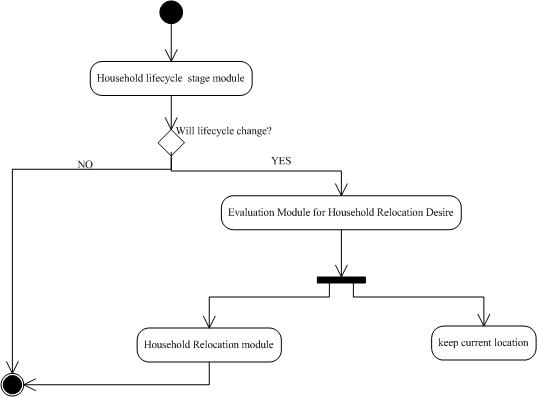
Figure 1. UML state diagram of the HRRM 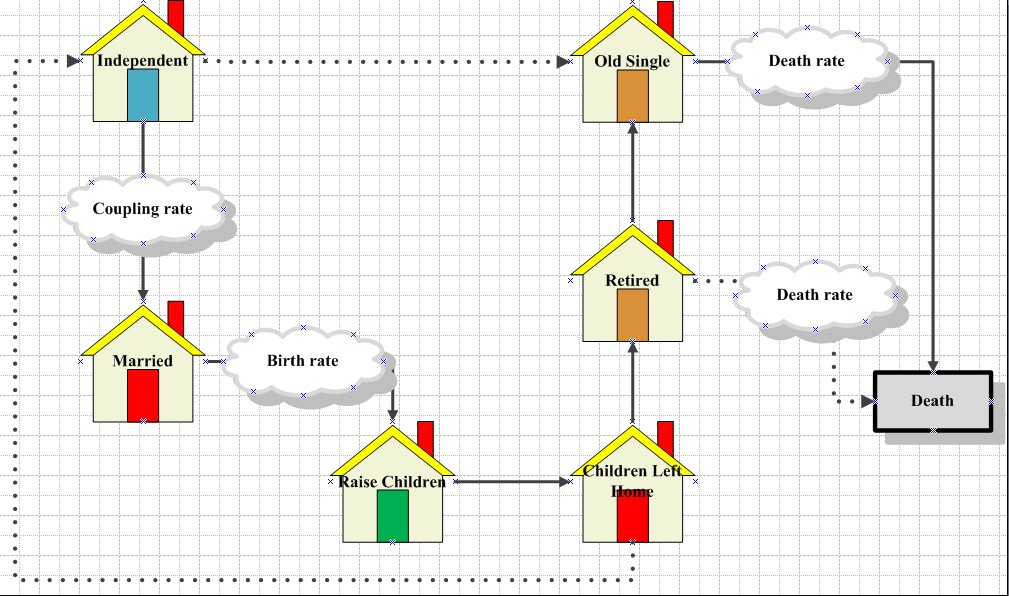
Figure 2. Diagram of the household lifecycle stage in the HRRM Household agent
- 2.2
- The HRRM is a spatially oriented agent-based model, in which there are household agents and urban space. Household agents represent the human population, and urban space (i.e. land units) represents the space where people live. In the HRRM, people correspond not to individual agents in the virtual city, but rather to members of households. A household is an agent, which is a coherent unit of simulation in the HRRM, that can make decisions as a single entity. This single entity is assumed to be composed of a family consisting of one or more people. In the HRRM, the household agent has such attributes as age, marriage status, members, deposit, income, and means of transportation.
- 2.3
- All of the household agents in the present simulation are designed to follow the lifecycle process presented in Fig. 2. We divided the total lifecycle of a household into seven stages in order to clarify the possibilities of relocation in each lifecycle stage. As shown in Fig. 2, in the first stage 'Independent', an independent household is created. After several years of independent, single life, the individual of this household meets someone and decides to get married. In the second stage 'Married', the couple finds a larger house, and a new household is formed. Though some households do not enter the second stage, a number of households will enter the third lifecycle stage. In the third stage 'Raise children', couples find that their current houses are too small or too far away from local schools, so they decide to relocate again. In the fourth stage 'Children leave house', a new generation of households is created, and, as shown by a dotted line, when a child in a household reaches 18 years of age, he or she will find a new residence and begin the first lifecycle stage of a new household. During this process, the individuals who remain in the old household continue to age and eventually retire. One of the individuals will eventually die, and the remaining individual becomes single again. Finally, the remaining individual will die and disappear from the simulation model.
Adaptive behaviours of household agents in the residential relocation process
Decision process for household relocation desire
- 2.4
- In the HRRM, we see that when the current lifecycle of a household agent moves to the next stage, the agent will decide on whether to move or not in order to adapt to the new life stage. This process we defined as household decision-making on residential relocation desire. For this process, a household's satisfaction with its current location and its ability to afford a new one are key. As shown in Fig. 3, a decision process is designed so that household agents will make relocation decisions during each lifecycle stage based on the age of the household. As shown in this figure, the household's satisfaction will first be evaluated in order to judge whether household agent i is satisfied with the current location or if relocation is desired. If the results indicate that satisfaction with the current location Si is below a satisfaction threshold, then household i will consider relocation. After the satisfaction estimation, household agent i predicts the expected costs of the desired relocation and then compares these costs with current savings. The household will relocate if these costs can be borne. Otherwise, the household must remain in its current location. Accordingly, the relocation process will be implemented by the household relocation choice module in the HRRM in order to decide where to relocate.
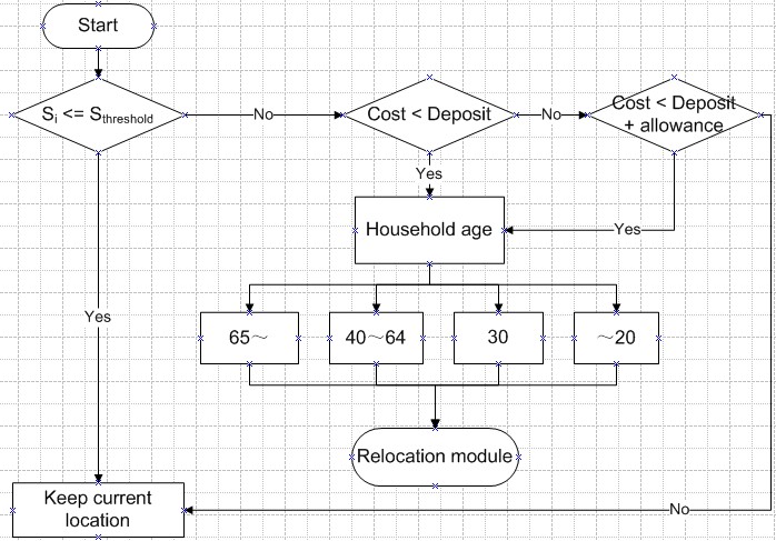
Figure 3. Decision process for household relocation desire Decision process for household relocation choice
- 2.5
- We assume that households belonging to the same age group exhibit similar utility preferences with respect to relocation. In this section, we propose that households which want to relocate will follow the decision-making flow shown in Fig. 4. Unlike some simulations that focus on residential sprawl (Vega and Reynolds-Feighan 2009; Li and Muller 2007; Brown and Robinson 2006), the present study attempts to reveal the effectiveness of a residence promotion policy for downtown revitalization. Thus, we consider the relocation process between downtown and other urban areas. As shown in Fig. 4, the urban areas are divided into three different regions. For each household agent, we assume that the residential utilities provided by different urban areas are different (the three regions), whereas the utilities are homogenous within one region, with a random range following a normal distribution that represents individual preferences. When households relocate, they must compare the different utilities of residential locations for adapting themselves to new locations based on the necessities of their new life stages. The alternative locations are randomly distributed within these three urban areas — i.e. the city centre area (CCA), the urban promoting area (UPA), and the urban control area (UCA). Based on this comparison, households will eventually choose an area that provides the greatest utility.
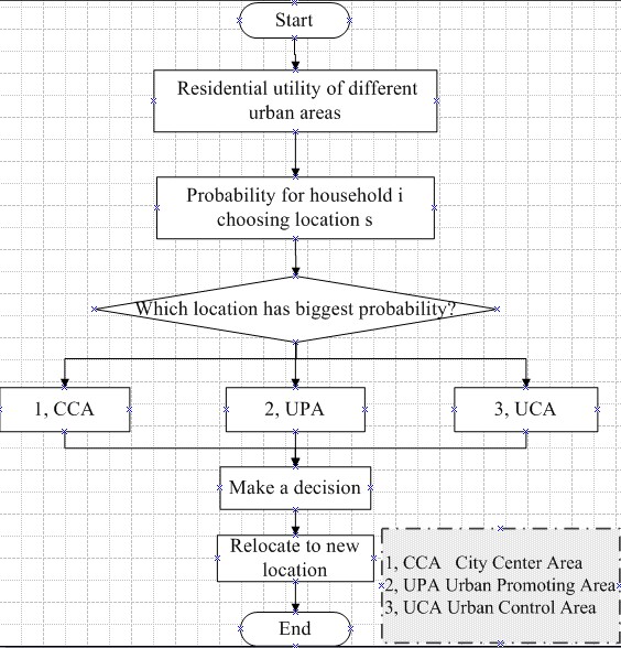
Figure 4. Decision process of household relocation choices Policy interactions between household agents in the residential relocation process
- 2.6
- Interactions between household agents are considered to take place in their adaptive behaviours during residential relocation process in response to the residential promotion policy. For representing the interactions in simulation, the interactions between household agents are designed as one component of the utility model. Although utility models are widely used in considering residential locations (Moeckel et al. 2007), the utility theory conventionally does not reflect the influences of neighbours. In the present study, the utility model is combined with the agent-based simulation in order to clarify the interactions between household agents in the residential relocation process during different lifecycle stages of households. In order to clarify the interactive influences between household agents regarding the residence promotion policy, interactions between household agents are designed to occur on two levels in the HRRM.
- 2.7
- We propose that household relocation behaviours will be influenced by the policy attitudes of households from the entire city and their neighbours, which are defined as household interactions at the global and neighbourhood levels — namely, global influence and neighbourhood influence. The global influence represents the policy attitude, which is the proportion of households in a city that accept and plan to use the local residence promotion policy for relocation. At the neighbourhood level, neighbourhood influence will be considered in order to represent the effect of neighbours on household residential relocation. It reflects the delivering of information about the policy by households within a small neighbourhood. The details of these two factors are explained below.
- Neighbourhood influence: the ratio of neighbours that use the residential allowance policy to relocate to a downtown area divided by the number of neighbours that do not use the policy for relocation. Here, neighbourhood influence can represent agent choices influenced by neighbours who plan to use the policy. This indicator is added to the utility model as an extra component of utility for reflecting interactions between neighbours. The neighbourhood is defined as the number of household agents within the nine cells of Moor neighbours in this work.
- Global influence: ratio of the total number of households that use the policy for relocation divided by the total number of households. This factor represents the proportion of households in the city that accept the policy and plan to use the policy for residential relocation to a downtown area. This indicator is also defined as one component of utility, which is the policy impact on individual relocation decisions from the entire city.
Models for adaptive behaviours of household agents in the residential relocation process
Household satisfaction with current location
- 2.8
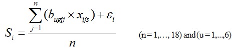
- When a household agent considers relocating, the final decision depends on the satisfaction level with the current location. However, a new household agent may find a new location without evaluating the satisfaction with the current location. In the HRRM, the satisfaction of a household with its current location can be evaluated based on the attributes of the household agents and spatial information — namely, the attributes of urban space. Each cell in an urban space has a series of predefined spatial attributes. The mathematical models used in the evaluation of household satisfaction with the current location are shown in the following equations:
(1) 
(2) 
(3) 
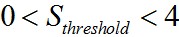
(4) where Si is the satisfaction of household i with the current residential location, bugij is a vector of retrospective coefficients to variable j, and u indicates the step of the lifecycle of household i in income group g. Here, xijs is the satisfaction of household i in location s produced by variable j and has four levels: 1) extremely unsatisfied, 2) unsatisfied, 3) satisfied, and 4) very satisfied. If one household agent's satisfaction with the current location is less than the Sthreshold, this agent will consider relocating. However, the decision to relocate will be made based on the utility of the relocation candidates.
Utility provided by urban space to household agents
- 2.9
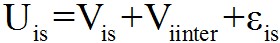
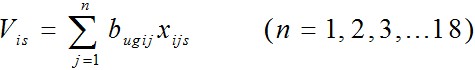
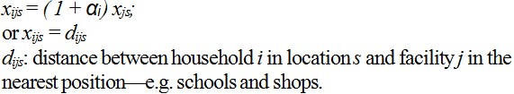
- Households make decisions on new locations based on the utility of the location. The utility model used to describe the subjective difference between the agent's choices is given in Eqs. 5 through 7. In Eq. 5 and 6, Vis is the utility of household i provided by location s without the unobserved random component and interaction between household agents Viinter. xijs is a vector of observable explanatory variable j describing the attributes of household i in location s. As shown in Eq. 7, xijs can be defined in two forms, one of which is the evaluation of household i of the spatial attribution xj in location s; another is the distance between household i in location s and public facility j in the nearest position — for example, schools, shops, and so on. For reflecting the difference of xijs between all household agents i in location s, a random number αi is generated, which follows normal distribution with a mean of 0 and a standard deviation of 0.1, as shown in Eq. 7.
- 2.10
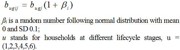
- In the present study, we observe the differences in residence utility preferences of households in different lifecycle stages. For this purpose, we set bugij as shown in Eq. 8 as coefficients of the observed components j to household i in the u lifecycle stage of the g income group. Utility preferences 1 through 6 are explained in Table 1, in which β is a random perturbation with a mean of 0 and a standard deviation of 0.1, generated with a normal distribution to represent individual preferences. Here, we use a decision rule as shown in Fig. 5 to determine different utility preferences between household agents in the HRRM.
- 2.11
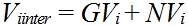
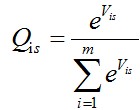
- In Eq. 9, Viinter stands for the interaction of household i with other household agents in urban space, which can be divided into the neighbourhood influence NVi and the global influence GVi of household agent i. In Eq. 10, NVi is defined as the ratio of neighbours that use the residential allowance policy to relocate to a downtown area Nmove divided by the number of neighbours that do not use the policy for relocation Nnomove. GVi is defined as ratio of the total number of households Gmove that use the policy for relocation divided by the total number of households GTotal. As shown by Eq. 11, component εis reflects the unobserved random contribution to utility Vis and Viinter. This random element εis follows a Gumble distribution and can be generated by Eq. 11, in which r follows a random uniform distribution, and constants μ and β are set to be -4.5 and 2, respectively, because it is preferable to fix the range of εis between -10 and 10. In addition, Qis is the probability of household i's choosing location s, which is in the form of Eq. 12.
(5) 
(6) 
(7) 
(8) 
(9) 
(10) 
(11) 
(12) 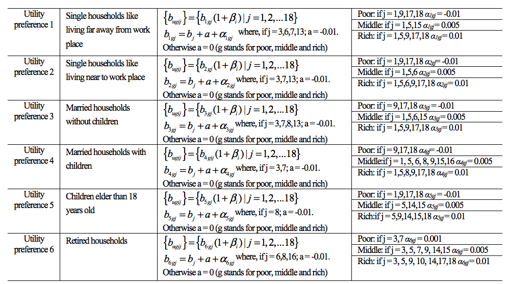
Table 1. Parameters for utility preference by households in different lifecycle stages 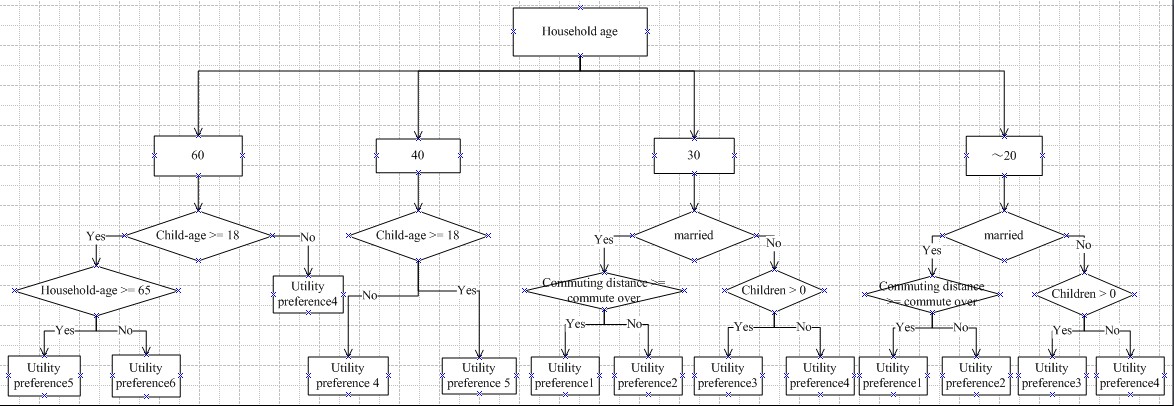
Figure 5. Residence utility preferences of households
Policy, Virtual Urban Space and Parameters for Simulation Configuration
-
Policy approach for downtown revitalization in Japan
- 3.1
- Generally, there are three stages of urban development (Klaassen and Paelinck 1979): urbanization, suburbanization, and urban decline. The social background regarding urbanization in Japan is introduced here briefly as relevant to this research. The residential population density in Japanese urban areas — such as Hokkaido, Honshu, Shikoku, and Kyushu — reached a maximum value of approximately 105.6 people per hectare in 1960 during rapid urbanization (Kaido 2005). The increased population density in the downtown areas, higher incomes, and generally cheaper transportation that resulted from this urbanization period led to increased housing demand in suburban areas. Although research has indicated that people in urban and suburban areas have differing circumstances, improvements in accessibility through the use of public transportation and private vehicles means that relocating to the suburbs is not expected to lead to inconvenient living conditions — i.e. less access to comfort (Marcellini 2007). Instead, home ownership can provide a feeling of security to people who are not financially well off (Rogers 1999). Thus, the residential population density rate in Japanese city centres has decreased overall since the 1980s. In particular, as it has been proven that an increase in commuting distance will not necessarily result in a significant increase in commuting time because of developments in transport technology (Ma and Kang 2010; Kim 2008; Schafer 2000), living in the downtown is not as attractive as before. This situation differs in small cities versus big metropolitan areas; for example, the Tokyo Metropolitan Area experienced suburbanization after 1965 while its total population continued to increase in the 1980s (Okamoto 1997). However, smaller cities in Japan began to lose population toward the end of the 1980s, entering an era of urban decline.
- 3.2
- In Japan, local governments are increasingly interested in using policy approaches to revitalize their downtown areas and make their cities more compact. Some of these policy approaches have involved downtown regeneration efforts, including development controls on large-scale shopping centres (Shen et al. 2011). In some local cities of Japan, such as Kanazawa City, a residence promotion policy has been implemented in order to revitalize its downtown areas by encouraging households to relocate to downtown areas. The main strategy of this policy is to provide residents who relocate to downtown areas with local housing allowances. The details of this residence promotion policy in Kanazawa City (issued in 2005) are shown in Table 2. This policy is the background of our work in focusing on designing a model — namely, the HRRM — to simulate policy impacts on downtown revitalization.
Table 2: Residence promotion policy of Kanazawa City Building Types Utilization types Allowances House Buy new house Single household 10 % payment, 2 million JPY Two households 10% payment, less than 3million JPY Buy or repair old house Basic part+ supplementary part, less than 500,000+200,000 JPY Apartment Buy new apartment Basic part (5% of payment) + supplementary part (1%), less than 1 million + 200,000 JPY Old apartment Buy Repair 50% of design payment, less than 1 million JPY Virtual urban space for accommodating household agents
- 3.3
- In order to simulate the effects of the residence promotion policy on downtown revitalization, we designed a virtual space that reproduces the urban planning conditions of a typical Japanese city. In Japan, cities that implement city planning laws are referred to as delineation cities (DCs), where an urbanization control line (UCL) is established in order to divide the urban planning area into UPA and UCA. The UPA is the area in which the local government is willing to promote urbanization through land-use zoning. The UCA is the area in which urbanization must be constrained. Land-use zones are further classified into three major groups: residential use, commercial use, and industrial use, which can be further broken down into 12 more detailed categories of land-use zones. The proposed model assumes that the virtual urban space (patch data) has the typical characteristics of delineation cities in Japan: it has 1) a traditional CCA located in the heart of the city, 2) an urban planning area divided into the UPA and the UCA, and 3) defined land-use zones within the UPA. In this work, we embody the concepts of the typical local city of Japan in a mono-central virtual space as shown in Fig. 6. The virtual urban space consists of 2,500 cells (50 × 50) where each cell measures 500 m × 500 m. In addition to the planning information, each cell in the virtual urban space will have predefined spatial attributes, such as shopping area, green space.
- 3.4
- It is impossible, however, to generate a typical Japanese city in space without including numeric information, such as the sizes of CCA, UPA, and UCA, and household density. For this reason, we referred to Kanazawa City, a typical Japanese local city, for organizing the virtual urban space in the present work. As shown in Table 3, the attributes of the virtual space planning areas, including the areas of land use zoning, are based on the situation of Kanazawa City. The global parameters, including birth rate, death rate, and coupling rate are based on the Basic Census Survey of Kanazawa City (2005-2007). With respect to the attributes of households, the household locations in this virtual city follow the household densities in the land-use zoning and residential suitability restrictions of Japan. Households are further grouped into three income levels: rich, middle class, and poor. We set the percentages of population belonging to the three income levels at 20%, 60%, and 20%, respectively, allocating them in the virtual space according to the percentage of income groups in the different land use zoning areas of Kanazawa City. With respect to the number of households, 1,500 household agents were initially generated in this virtual city according to household density defined by planning regulation — i.e. the floor area ratios in different land use zones. Accordingly, household density in the virtual urban space has been created as shown in the third image from the left in Fig. 6, and household income is represented in the right-most image of Fig. 6. We also assume that all households have cars. In the present research, the designed virtual urban space and agent distributions have already been utilized by Shen et al. (2011).
- 3.5
- Furthermore, each cell of this virtual space has 18 spatial attributes (x1 through x18). These features will be used by household agents to evaluate their satisfaction with current locations or to make relocation choices. A detailed introduction of the 18 spatial features is given in Table 4. The 18 features at the cell level of the virtual city are divided into two groups. One group consists of objective features, such as the distribution of public facilities, and we marked these objective features in the virtual city. The other group consists of subjective features that we cannot mark in the space. These subjective features are randomly valued at a certain rank following certain rules, as introduced in Table 4, based on the general situation of a typical Japanese city.
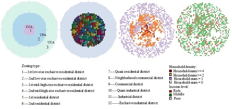
Figure 6. Virtual urban space for accommodating household agents Table 3: Global parameters, Attributes of virtual space and household agents Parameter name Predefined data Global parameters Birth rate 0.90% Death rate 0.80% Coupling rate 0.59% Threshold for satisfaction 0.1, Kidani and Kawakami (1996) Policy scenario option Use residence promotion policy or not Commute-over Maximum commuting distance Attributes of Virtual space Land use zoning 12 types of land use zonings Household Density Household numbers based on Floor Area Ratios Based on land use zoning Planning areas CCA(4%), UPZ(32%), UCA(64%) 18 spatial featuress 18 variables (as Tab.5) evaluated based on location. House price 800 (CCA), 400(UPA), 200(UCA) thousands (JPY)/ 3.3 m2 Attributes of Household Income Low(20%), middle (60%) and high (20%) Car ship Yes Household age according to household lifecycle stages described in Fig. 2 Family members 1 - 6 based on lifecycle stages Saving Random Number based on income groups and lifecycle stages Global influence As described in section 2.4 Neighborhood influence As described in section 2.4 Personal Satisfaction threshold The global threshold 0.1 and a random number in normal distribution with mean 0 and SD 0.01. Satisfaction of current location As described in section 2.5.1 Individual parameters of Utilities regarding relocation alternatives As described in Table 5. Location Coordination x, y 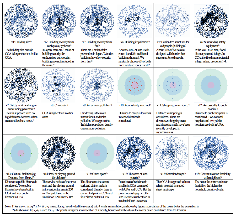
Table 4. The spatial features of the virtual city for households' making decision on residential relocation choices Parameters for simulation of households' adaptive behaviours and policy interactions on residential relocation
- 3.6
- The parameters of the utility model in the present work represent the principles of adaptive behaviours and policy interactions of household agents in a residential relocation process. Those parameters are retrieved from the results of an empirical survey in Kanazawa City in order to associate the preferences of household agents in real society with those in the virtual space. The empirical survey focused on two parts: 1) satisfaction with current locations and 2) knowledge of local residence promotion policy. For the first theme, the questionnaire asks the question, 'Would you like to relocate?' Based on the results of the survey, we estimated the parameters through a regression analysis of Si and xijs, using R statistical software to determine the coefficients bj (b1 to b18) for household agents' evaluation of satisfaction with their current locations. These results are listed in Table 5. For the second focus, the questionnaire asks the question, 'Do you plan to relocate to a downtown area as a result of this policy and in doing so receive an allowance?' Residents were asked to choose an answer from among four options. A regression analysis was conducted in order to estimate the coefficients representing the policy effects on household relocation based on the questionnaire. These estimated partial coefficients are listed in Table 5 as b'j. In addition, the HRRM was implemented on the Netlogo platform for model testing.
Table 5: Partial correlation coefficient of impact factors on household relocation utility and satisfaction Variables for satisfaction evaluation Coefficients (bj) Partial coefficient
(no policy interaction)Significant Coefficients(b'j) Partial coefficient
(with policy interaction)Significant x1: Building size b1 0.170634 **** b'1 0.069904 · x2: Building security from earthquake, typhoon b2 0.140753 **** b'2 0.153358 *** x3: Building security from fire b3 0.045609 · b'3 0.085280 * x4: Building impairment b4 0.029561 · b'4 0.112268 ** x5: Barrier-free structures for old people b5 0.067244 · b'5 0.051591 · x6: Surrounding safety equipments b6 0.125595 *** b'6 0.072290 * x7: Safety while walking on surrounding pavement b7 0.126829 *** b'7 0.105173 * x8: Crime rate b8 0.109048 *** b'8 0.085835 * x9: Air or noise pollution b9 0.162371 **** b'9 0.098698 * x10: Accessibility to work or school b10 0.056896 · b'10 0.079705 * x11: Shopping convenience b11 0.118102 *** b'11 0.075495 * x12: Accessibility to community hospital b12 0.111277 *** b'12 0.052196 · x13: Cultural facilities (e.g. Distance from library) b13 0.097474 ** b'13 0.058622 · x14: Park or playing ground for children b14 0.100275 ** b'14 0.100814 * x15: Green space b15 0.079093 ** b'15 0.123672 ** x16: The areas of out space b16 0.172469 **** b'16 0.027558 · x17: Street landscape b17 0.087435 ** b'17 0.102831 * x18: Communication feasibility with neighbors b18 0.061328 · b'18 0.020922 · Interaction 1: Neighborhood influence (x19) b'19 0.064556 · Interaction 2: Global influence (x20) b'20 0.174542 **** Significant values: 0.1 " · " 0.05 "*" 0.001 "**" 0.0005 "***" 0.00001 "****"
Model Test
-
Sensitivity test for households' adaptive behaviour in a residential relocation process
- 4.1
- In the HRRM, the adaptive behaviours of household agents in a residential relocation process were developed using a lifecycle stage model and a utility model as introduced in section 2; therefore, it was necessary to prove that adaptive behaviours based on these models in the HRRM could produce reasonable simulation outputs. For this purpose, we conducted a sensitivity analysis of the parameters relating to adaptive behaviours (e.g. satisfaction threshold, parameters of lifecycle stages) and policy interactions. The interface of the HRRM is shown in Fig. 7. One tick in the simulation represents one year, and 30 ticks are simulated in each experiment. The simulation results thus represent the results for 30 years, following from the initial stage. The entire sensitivity test was repeated in 50 experiments with the initial values of the parameters listed in Tables 3 and 5, but the parameter tested changed according to the needs of the sensitivity analysis.
Satisfaction threshold and desire of a household to relocate
- 4.2
- In Fig. 8(a), we show the sensitivity test of the satisfaction threshold households use to evaluate their current residential location. We tested our model by adjusting the satisfaction threshold from -0.9 at the first tick to 1.2 at the 210th tick by means of setting the tick interval to 0.01. As shown in Fig. 8(a), the number of households satisfied with their current location decreases as the threshold increases. The number of households satisfied with their current location and the number that are dissatisfied intersect when the threshold value is 0.25 at the 115th tick, and the intersection corresponds to the threshold 0.25, at which the proportion of households that are satisfied with their current location is 50%. Previous studies have revealed that, in Kanazawa City, the proportion of households that wish to relocate is 30% (Kikuchi and Nojima 2007; Kawakami and Takama 1978). Thus, we set the satisfaction threshold of household residential relocation as 0.1 in order that the ratio of 'unsatisfied' household agents will remain around 30% in simulation, as shown in Fig. 8(b).
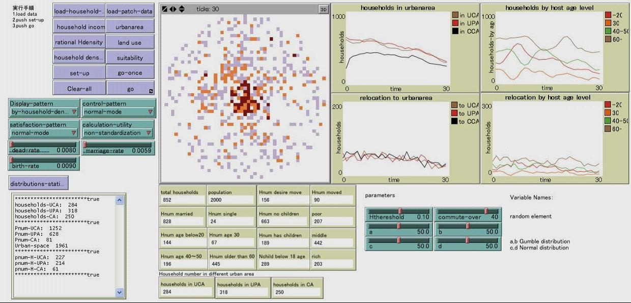
Figure 7. Interface of the HRRM in the Netlogo platform .png)
.jpg)
a) Sthreshold (-0.9 to 1.20) (b) Sthreshold = 0.10 Figure 8. Satisfaction threshold influence on the desire of households to relocate Test on the parameters of household lifecycle stage
- 4.3
- The number of household agents in the urban space changes based on the changes of parameters relating to the lifecycle stages. In order to investigate how the relocation process is influenced by the lifecycle stage, a sensitivity test was conducted of such parameters as the birth rate and death rate as defined in the lifecycle stage. We conducted 50 experiments in which the birth rate and death rate were varied in order to determine the sensitivity of the effects of the two parameters on household residential relocations. In Fig. 9(a1) and (a2), the birth rate was set to 0.1 and 0.5, respectively. First, a sensitivity analysis of the birth rate was conducted. The death rate and coupling rate were maintained constant at their initial values. As shown in Fig. 9(a1), there are more households in the UCA than in the CCA during the running of the simulations. As the birth rate grew to 0.5, the numbers of households in the three urban areas increased while maintaining the same relative relationship in Fig. 9(a2).
- 4.4
- The figures through Fig. 9(b1) and (b2) represent households that relocate to different urban areas. As the birth rate increases, although the total number of households that relocate to different urban areas eventually increases, most of these households relocate to the UCA. In the meantime, we further used images to show the average value of relocated households at different age levels. One thing should be clarified here is that the household age we talked here are the ages of householders. As shown in Fig. 9(c1), when the birth rate equates to 0.1, most relocations occur among households that are more than 60 years old, followed by households between 40 and 50 years old. Households younger than 20 (around 18) or approximately 30 years old show a low potential for relocation. When the birth rate is increased to 0.5, however, the trend gradually changes; most relocations happen among households younger than 20 years old. The sharp increase in the birth rate will increase the percentage of young households in the population, thereby resulting in an increase of relocations among households less than 20 years old. Thus, a higher birth rate results in increasing the number of young households (less than 20 years old). From this viewpoint, although a higher birth rate can relieve the situation of an aged society, it will not increase the residential rate in urban centres, as indicated in the simulated result in Fig. 9(b2). Therefore, without special policies, downtown areas will not be revitalized even though the total number of households is increasing.
- 4.5
- In contrast, if we keep the birth rate constant at its initial value but increase the death rate from 0.008 to 0.1, as shown as Fig. 10(a1), both the total number of households and the numbers of households in different urban areas decrease. The increased death rate does not change the trend of household relocation with respect to age levels in Fig. 10(a2). Households that are more than 60 years old make up the majority of households that relocate. Furthermore, a minority of households that are approximately 30 years old, along with most other households, relocate to the UCA. This helps to clarify the situation of local urban decline and the aged society. Without increasing the birth rate, the death rate has no obvious effect on downtown decline or the aged society. Moreover, without special intervention with the goal of downtown revitalization, changes in the birth rate or the death rate do not influence downtown decline. Although increasing the birth rate can increase the number of young households and improve the relocation frequency, most relocations still occur in the UCA.
- 4.6
- As a result, we can conclude that in the HRRM, the changes in the parameters of the lifecycle stage can produce reasonable changes in household adaptive behaviours in residential relocation, but it is impossible to revitalize the downtown. In order to increase the relocation frequency to CCA, special policy intervention is needed. In the following section, we will investigate policy impacts on the relocation of household agents through agents' interactions.
.jpg)
.jpg)
(a1) Households in urban area by birthrate 0.1 (a2) Households in urban area by birthrate 0.5 .jpg)
.jpg)
(b1) Households relocation to urban area by birthrate 0.1 (b2) Households relocation to urban area by birthrate 0.5 .jpg)
.jpg)
(c1) Households relocation by host age by birthrate 0.1 (c2) Households relocation by host age by birthrate 0.5 Figure 9. Household change in different urban areas according to birth rate .jpg)
.jpg)
(a1) Households in urban areas by death rate 0.008 (a2) Households in urban areas by death rate 0.1 .jpg)
.jpg)
(b1) Households relocation to urban area by death rate 0.008 (b2) Households relocation to urban area by death rate 0.1 .jpg)
.jpg)
(c1) Households relocation by host age by death rate 0.008 (c2) Households relocation by host age by death rate 0.1 Figure 10. Household change in different urban areas according to death rate Policy impact on households' decision making concerning the residential relocation process
- 4.7
- As shown in Fig. 3, household agents who have a desire to relocate will compare the relocation costs with their savings. If household savings are insufficient, the household will consider applying for the allowance stipulated in the local residence promotion policy and will relocate to a downtown area rather than simply to the area with the highest utility.
- 4.8
- In order to investigate the policy impact on the decision of household agents in the household relocation process, a sensitivity analysis was conducted on neighbourhood influence and global influence, which are related to the ratio of agents who agree to take advantage of the policy and relocate to a downtown area. First, we tested the model with the neighbourhood influence as 0.064556 and global influence as 0.174542 (estimated results in Table 5), which are the initial values and named initial interactions in Fig. 11. We then changed the values of neighbourhood influence and global influence both to 0.5 to show the changes in household residential relocations during an increase in policy interactions. Thereafter, we conducted a comparative analysis between the simulation results with initial policy interactions and the results with increased policy interactions by means of R software. During all these processes, all other parameters of HRRM were maintained constant at their initial values.
- 4.9
- If Fig. 11(a1) is compared with Fig. 9(a1) or Fig. 10(a1), it can be seen that when the policy interaction was incorporated in the simulation, the number of households in the CCA increased (as shown by the gray). Meanwhile, Fig. 11(b1) shows that the number of households that relocated to the CCA also increased correspondingly. This result shows that households would be affected by this residence promotion policy during their decision-making on residential relocations if the policy was publicized within the neighbourhood and entire society. Figs. 11(c1), 9(c1), and Fig 10 (c1), however, show that the most relocations occurred among households that are more than 60 years old, followed by households between 40 and 50 years old, households that are younger than 20 (around 18) and households that are approximately 30 years old, in that order. These results would seem to indicate that the trend of households doing relocations in different age groups will not change whether there is a policy intervention or not. Next, we further investigated how household relocation would change if we changed the intensity of the policy impact on household interaction.
- 4.10
- Thus, we increased the neighbourhood influence and global influence to 0.5. The comparative simulation results are shown in Figs. 11 (a2), (b2), and (c2). The virtual urban space in the present work was designed as a closed urban space without population mobility from the outside. This situation decreases the total number of households during simulation. When neighbourhood influence and global influence are both 0.5, the gray boxes in Fig. 11(a2), which represent the number of households in the CCA, further increase, but the household density in the UCA and UPA decreases significantly. The decrease in the number of households in the UCA and UPA is partially a result of the decrease in the total number of households, and the increase in the number of households in the CCA is a result of the residence promotion policy. In addition, as the values of neighbourhood influence and global influence increase, the number of households in the CCA increases obviously in Fig. 11(b2) compared with Fig. 11(b1); specifically, the number of households that relocate to the CCA increases in both of these figures. These results do indicate that a residence promotion policy can influence household residential relocation to a downtown area and that the HRRM can represent and visualize this process.
.jpg)
.jpg)
(a1) Household number in urban areas with initial interactions (a2) Households in urban area with increased interactions .jpg)
.jpg)
(b1) Households relocation to urban area with initial interactions (b2) Households relocation to urbanarea with increased interactions .jpg)
.jpg)
(c1) Households relocation by host age with initial interactions (c2) Households relocation by host age with increased interactions Figure 11. Household change in different urban areas according to policy interactions - 4.11
- However, as indicated by Figs. 11(c1) and (c2), as with the birth rate and death rate sensitivity analyses, the number of households that relocated to the CCA are, in decreasing order, households that are more than 60 years old, households that are between 40 and 50 years old, households that are approximately 20 years old, and households that are approximately 30 years old. Thus, we can conclude that the limited allowances for relocation are not sufficient to encourage younger households to choose residences in downtown areas. As shown by Fig. 10(c1) and (c2) and Fig. 11(c1) and (c2), the middle-aged and elderly households are both more likely to relocate to a downtown area using this policy, as compared to households that are less than 30 years old. Therefore, this policy probably tends to be more attractive to households more than 40 years old that are well-off. From this viewpoint, good publicizing of the residence promotion policy have an effect on households relocating to downtown, but this effect is limited.
The Moore Test for Spatial Repeatability
- 4.12
- From Figs. 9 to 11, we can confirm that the number of household agents and relocations are statistically stable in the 50 times simulation results. In this section, we would like to further prove the spatial repeatability of simulation results by means of the HRRM. The experiments were done 50 times with the parameters introduced in Tables 3 and 5. In each experiment, we ran the simulation for 30 ticks. Simulation results taken every 10 ticks were used to determine the spatial repeatability of the number of households in each cell for the same tick number among the 50 simulations.
- 4.13
- First, the means among the 50 simulations of the numbers of households for a cell at 10, 20, and 30 ticks are visualized, as shown in Fig. 12. A Welch's t test of the number of households for different simulations was conducted, and Sig. was less than 0.05 in all cases. Thus, the simulation results obtained using the HRRM are stable. We also conducted a Moore Test of the number of households in each cell using R; the results revealed a stable correlation and showed that Sig. was less than 0.05 in all cases.
- 4.14
- Summarizing the sensitivity analysis in Section 4, when we adjust the parameters related to lifecycle stage and household interactions, the HRRM can reflect reasonably well the changes in the number of households in different urban areas. Moreover, the spatial distribution of household agents in the simulation process is repeatable, too.
.jpg)
.jpg)
.jpg)
(a) Average agent number in each cell at tick 10 (b) Average agent number in each cell at tick 20 (c) Average agent number in each cell at tick 30 Figure 12. Household distribution in virtual urban space in simulation process
Note: A Welch's t test and a Moore Test have been conducted for numbers of households between ticks 10, 20, and 30. Significance is smaller than 0.05 in all casesComparing simulation data and real data for Kawakawa City
- 4.15
- Following the explanation in subsection 3.2, we designed the virtual urban space based on the situation of a typical Japanese city. Specifically, we retrieved parameters from an empirical survey of Kanazawa City in order to associate the behaviour preferences of household agents in simulation with those of a typical Japanese city. Thus, the simulated population distribution of the HRRM is expected to be similar to the characteristics of Kanazawa City. As mentioned in Subsection 3.2, even though urban spaces and population distributions of different planning areas in virtual space and those of Kanazawa City are different, we assume that household agents will compare the utilities only between alternatives selected randomly from the UPA, UCA, and CCA. Thus, in the present study, it is possible to compare the proportions of household numbers in different planning areas between the virtual space and Kanazawa City.
- 4.16
- Consequently, the simulation of household residential relocation using a virtual space was designed for 15 years. In order to make a comparison with 1985-2000 in Kanazawa City, we compared the simulation results with local statistical data by converting the simulation results into household ratios for different urban planning areas. The results are compared in Table 6, which shows that the local census survey in 1985 gives household ratios of 33.9% in CCA and 66.1% in UPA and UCA, whereas the respective values obtained by the simulation are 32.7% and 67.3%. Thus, the simulation results are in good agreement with the real data. Up until 1990, the household ratio in CCA was 31.9% for the real dataset and 32.1% for the simulation, which again agree well. This is also the case for 1995. However, the difference became larger in the year 2000: the simulation results for households in CCA are 10% greater than in the real data. This result probably stems from a change in the Building Standards Act in 1998, in which the traditional six types of land-use zones were changed to 12 types of land-use zones (Building Standards Act 1998).
Table 6: Comparison of household ratios in different urban areas between real data and the simulation results Years: 1985 1990 1995 2000 Real dataset CCA 33.9% 31.9% 29.0% 26.6% UPA+UCA 66.1% 68.1% 71.0% 73.4% Simulated results CCA 32.7% 32.1% 30.4% 33.7% UPA+UCA 67.3% 67.9% 69.6% 66.3%
Conclusions
- 5.1
- The HRRM integrated the adaptive behaviours and policy interactions of household agents in a residential relocation process, which can mimic the process of household decision-making in residential relocation by integrating ABM with household lifecycle stages, satisfaction evaluation of the current residential location, and selection of a new location.
- 5.2
- Regarding the evaluation module for household relocation desire and choice in the household relocation process, we developed a utility model to reflect individual choices by introducing a normally distributed random perturbation to the partial correlation coefficients of all variables in the utility model, which can be recognized as the preference of households for adapting themselves to different locations in new lifecycle stages in the HRRM. Interactions between household agents are considered to take place at the levels of the neighbourhood and the entire city, reflecting their attitudes to the residence promotion policy during the residential relocation process, which were included as one component of utility model.
- 5.3
- In order to test the adaptive behaviours and interactions of household agents in simulation, we examined the model's sensitivity to the parameters defined in the lifecycle stage module and the parameters defined in household policy interaction. Comparing the simulation results with different policy parameters, it was determined that the number of households relocating to the CCA increases when the policy parameters are introduced. This means that downtown decline can be relieved by implementing this residential policy as modelled here. Although the local residence promotion policy affects household residential relocation to a downtown area, the policy is not very effective either for households that are younger than 20 years old or for households that are approximately 30 years old. Thus, we analyzed whether the allowance for relocation was insufficient for encouraging younger households to choose residences in downtown areas and found that this policy tends to be more attractive to well-off households — that is, those that have sufficient savings to relocate. Compared to households less than 30 years old, middle-aged households and elderly households both exhibited a greater tendency to relocate to downtown areas using this policy.
- 5.4
- The parameters employed for the virtual space are based on the situation of Kanazawa City, and the parameters of the utility model are estimated based on responses to an empirical survey conducted in Kanazawa City. Thus, the parameter values used in the HRRM can be associated with those in Kanazawa City. Finally, we compared the simulation results obtained using the HRRM and the real statistical data for Kanazawa City, which revealed that the simulation results for the household residential relocation are similar to the real statistical results for actual household residential locations over the past 20 years in Kanazawa City. Thus, the HRRM can visualize the possible results of policy implementation, thereby making it possible to judge the potential effectiveness of a residence policy for revitalizing the city centre of a typical city in Japan.
References
-
ANTROP M. (2004). Landscape change and the urbanization process in Europe. Landscape and Urban Planning, 67, 9-26. [doi:10.1016/S0169-2046(03)00026-4]
BERGER T., Schreinemachers P., Woelcke J. (2006). Multi-agent simulation for the targeting of development policies in less-favored areas. Agricultural Systems, 88(1), 28-43. [doi:10.1016/j.agsy.2005.06.002]
BANISTER D. (1997). Reducing the need to travel. Environment and Planning B: Planning and Design, 24(3), 437-449. [doi:10.1068/b240437]
BANISTER D., Watson S. and Wood C. (1997). Sustainable cities: transport, energy, and urban form. Environment and Planning B: Planning and Design, 24(1), 125-143. [doi:10.1068/b240125]
BROWN D. G. and Robinson D.T. (2006). Effects of Heterogeneity in Residential Preferences on an Agent-Based Model of Urban Sprawl. Ecology and Society, 11(1), 46-67.
BENENSON, I. (1998). Multi-agent simulations of residential dynamics in the city. Computers, Environment and Urban Systems, 22, 25-42. [doi:10.1016/S0198-9715(98)00017-9]
BUILDING Standards Act. (1998). Ministry of Land, Infrastructure, Transport and Tourism, Japan. Japanese website Archived at: http://www.mlit.go.jp/
BOYLE, P., Halfacree, K., & Robinson, V. (1998). Exploring contemporary migration. Harlow, New York: Longman.
CADWALLER, M. (1992). Migration and residential mobility. Micro and macro approaches. Wisconsin: University of Wisconsin Press.
CLARK, W. A. V., & Onaka, J. L. (1983). Life cycle and housing adjustment as explanations of residential mobility. Urban Studies, 20(1), 47-57. [doi:10.1080/713703176]
DAWN C. P. and Filatova T. (2008). A conceptual design for a bilateral agent-based land market with heterogeneous economic agents. Computers, Environment and Urban Systems, 32, 454-463. [doi:10.1016/j.compenvurbsys.2008.09.012]
DIAPPI L. and Bolchi P. (2006). Gentrification Waves in the Inner-City of Milan - A multi agent / cellular automata model based on Smith's Rent Gap theory, Van Leeuwen, J.P. and H.J.P. Timmermans (eds.). Innovations in Design & Decision Support Systems in Architecture and Urban Planning (pp. 187-201), Dordrecht: Springer.
ETTEMA D. (2011). A multi-agent model of urban processes: Modelling relocation processes and price setting in housing markets. Computers, Environment and Urban Systems, 35, 1-11. [doi:10.1016/j.compenvurbsys.2010.06.005]
ETTEMA, D., de Jong, K., Timmermans, H., & Bakema, A. (2006). PUMA: Multi-agent modelling of urban systems. In E. Koomen, A. Bakema, J. Stillwell, & H. Scholten (Eds.), Land use modeling. Springer.
FONTAINE C.M., Rounsevell M.D.A. (2009). An agent-based approach to model future residential pressure on a regional landscape. Landscape Ecological, 24, 1237-1254. [doi:10.1007/s10980-009-9378-0]
HAASE D., Lautenbach S., Seppelt R. (2010). Modeling and simulating residential mobility in a shrinking city using an agent-based approach. Environmental Modelling & Software, 4,1225-1240. [doi:10.1016/j.envsoft.2010.04.009]
HOWLEY P., Scott M., Redmond D. (2009). An examination of residential preferences for less sustainable housing: Exploring future mobility among Dublin central city residents. Cities, 26, 1-8. [doi:10.1016/j.cities.2008.10.001]
JAGER W., Mosler. H. J. (2007). Simulating Human Behavior for Understanding and Managing Environmental Resource Use. Journal of Social Issues, 63(1), 97-116. [doi:10.1111/j.1540-4560.2007.00498.x]
KAZEPOV Y. (2005). Cities of Europe: Changing Contexts, Local Arrangements, and the Challenge to Social Cohesion. UK: Blackwell Publishing. [doi:10.1002/9780470694046]
KAWAKAMI M., Takama C. (1978). Investigation of household residential relocation desire in Kanazawa City (in Japanese). Architecture Institute of Japan, 13, 67-72
KIKUCHI Y., Nojima S. (2007). Resident's Mind about Residence Selection in Suburban Housing Estates: Case study of 4 suburban estates in Fukui City. City planning review: Special issue on city planning, 42(3), 217-222.
KIM C. (2008). Commuting time stability: a test of a co-location hypothesis. Transportation Research A, 42, 524-544. [doi:10.1016/j.tra.2008.01.001]
KAIDO K. (2005). Urban densities and local facility accessibility in principal Japanese cities, In: M. Jenks and N. Dempsey (Eds.), Future Forms and Design for Sustainable Cities (pp. 311-337). Architectural Press.
KLAASSEN, L. and Paelinck J. (1979). The feature of the large towns. Environment and Panning A, 11, 1095-1104. [doi:10.1068/a111095]
KIM, J.H., Pagliara, F., Preston, J. (2005). The intention to move and residential location choice behaviour. Urban Studies, 42 (9), 1621-1636. [doi:10.1080/00420980500185611]
KIDANI H, Kawakami M, 1996, "Actual condition and planning theme of building activity in urbanization control area" Journal of the City Planning Institute of Japan, 31, 583-588.
KULU, H. (2007). Fertility and spatial mobility: Evidence from Austria. Environment and Planning A, 40(3), 632-652. [doi:10.1068/a3914]
KULU, H., & Milewski, N. (2007). Family change and migration in the life course: An introduction. Demographic Research, 17(9), 567-590. [doi:10.4054/DemRes.2007.17.19]
KÄHRIK A., Leetmaa K., Tammaru T. (2012). Residential decision-making and satisfaction among new suburbanites in the Tallinn urban region, Estonia. Cities, 29, 49-58. [doi:10.1016/j.cities.2011.07.005]
LEE Q., Park B., Vlek S. J. P.L.G. (2010). Land Use Dynamic Simulator (LUDAS): A multi-agent system model for simulating spatio-temporal dynamics of coupled human-landscape system: 2. Scenario-based application for impact assessment of land-use policies. Ecological Informatics, 5(3), 203-221. [doi:10.1016/j.ecoinf.2010.02.001]
LI Y. and Muller B. (2007). Residential location and the biophysical environment: exurban development agents in a heterogeneous landscape. Environment and Planning B: Planning and Design, 34, 279 -295. [doi:10.1068/b31182]
MARCELLINI F., et al. (2007). Aging in Italy: Urban-rural differences. Archives of Gerontology and Geriatrics, 44, 243-260. [doi:10.1016/j.archger.2006.05.004]
MA K.R. and Kang E.T. (2010). Time-space convergence and urban decentralisation. Journal of Transport Geography, in press.
MOECKEL R., Schwarze B., Spiekermann K., Wegener M (2007) Simulating interactions between land use, transport and environment. Paper presented at 11th world conference on transport research. University of California. Berkeley, 24-28 Jun 2007
MOLIN, E., Timmermans, H. (2003). Accessibility considerations in residential choice decisions: accumulated evidence from the Benelux. TRB 2003 Annual Meeting CD-ROM, Washington, DC.
MILLER, E. J., Hunt, J. D., Abraham, J. E., & Salvini, P. A. (2004). Microsimulating urban systems. Computers, Environment and Urban Systems, 28, 9-44. [doi:10.1016/S0198-9715(02)00044-3]
MOECKEL, R., Wegener, M., & Schwarze, B. (2005). Simulating land use change by modelling persons, households and dwellings. In Paper presented at CUPUM conference, London.
MOECKEL R., Spiekermann K., Schürmann Carsten., Wegener M., (2003). Microsimulation of Land Use. International Journal of Urban Sciences, 7(1), 14-31. [doi:10.1080/12265934.2003.9693520]
MULDER, C. H., & Wagner, M. (1998). First-time home-ownership in the family life course: A West German/Dutch comparison. Urban Studies, 35(4), 687-713. [doi:10.1080/0042098984709]
NEWMAN P. and Kenworthy J. (1989). Cities and Automobile Dependence: An International Sourcebook. Aldershot: Gower Publishing Company.
NOTH, M., Borning, A., Waddell, P. (2003). An extensible, modular architecture for simulating urban development, transportation, and environmental impacts. Computers, Environment and Urban Systems, 27(2), 181-203. [doi:10.1016/S0198-9715(01)00030-8]
OKAMOTO K. (1997). Suburbanization of Tokyo and The Daily Lives of Suburban People. In: P.P. Karan and K. S Kentucky (Eds.), The Japanese City (pp. 79-105). The University Press of Kentucky.
RIENIETS T. (2005). Shrinking cities - Growing Domain for Urban Planning? Available at: http://aarch.dk/fileadmin/grupper/institut_ii/PDF/paper_presentation_EURA2005.pdf
RIENIETS T. (2009). Shrinking cities: causes and effects of urban population losses in the twentieth century. Nature and Culture, 4(3), 231-254. [doi:10.3167/nc.2009.040302]
ROGERS C.C., (1999) Changes in the older population and implications for rural areas. Economic Research Service (Rural Development Research Report No. 90), U.S. Department of Agriculture, Washington, DC. Available from: http://www.ers.usda.gov/publications/rdrr90/i.
ROUWENDAL, J., Meijer, E. (2001). Preferences for housing, jobs, and commuting: a mixed logit analysis. Journal of Regional Science, 41 (3), 475-505. [doi:10.1111/0022-4146.00227]
SCHAFER A. (2000). Regularities in travel demand: an international perspective. Journal of Transportation Statistics, 3(3), 1-31.
SHEN Z.J., Yao X.A., Kawakami M., Chen P. (2011). Simulation spatial market share patterns for impacts analysis of large-scale shopping centers on downtown revitalization. Environment and Planning B: Planning and Design, 38,142-162. [doi:10.1068/b35138]
TORRENS P.M. .(2001). Can Geocomputation save urban simulation? Throw some agents into the mixture, simmer, and wait... University College of London, Center for Advanced Spatial Analysis, Working Paper series: Publication 32.
TIMMERMANS, H. J. P. (2003). The saga of integrated land use-transport modeling: How many more dreams before we wake up? In Paper presented at the 10th international conference on travel behaviour research, Lucerne, 10-15 August, 2003.
VEGA A. and Reynolds-Feighan A. (2009). A methodological framework for the study of residential location and travel-to-work mode choice under central and suburban employment destination patterns. Transportation Research Part A, 43, 401-419. [doi:10.1016/j.tra.2008.11.011]
WADDELL, P., Borning, A., Noth, M., Freier, N., Becke, M., & Ulfarsson, G. (2003). Microsimulation of urban development and location choices: Design and implementation of UrbanSim. Networks and Spatial Economics, 3, 43-67. [doi:10.1023/A:1022049000877]