
 Abstract
- We present Flora, a testbed that supports multidimensional fitness and resource modeling. Its main features are evaluation metrics related to population wellbeing, scalable representation of resource diversity, and composability of sociotechnical test scenarios through the TDI framework. We ran simulations to illustrate Flora's use in modeling the effects of using information infrastructures with different component systems. We analyzed the impact of hoarders in the absence of accounting systems, compared the performance of different decentralized currency systems in terms of accounting design features, and modeled the potential impact of reputation systems in deterring detrimental socioeconomic behavior. Among findings were the importance of having resource diversity as well as resources that each could target different fitness dimension needs; the inherent robustness of accounting systems that allow organizations to set budgets independently of centrally issued currency; and the greater effectiveness of buyer-screening compared to seller-screening as a means for influencing malevolent socioeconomic actors.
- Keywords:
- Simulation Testbed, Reputation Systems, Decentralized Currency, Modular Framework, Agent-Based Model
Introduction
- 1.1
- Grassroots or aid groups typically propose policies or systems to foster socioeconomic development efforts within a community or region. Examples of such systems include mobile banking, public health information systems, and new educational programs. Another example is the proliferation of community currencies in Argentina when the national currency collapsed (Gomez 2010). Fair Trade and organic certification may also be considered as systems to help farmers gain better livelihoods and maintain sustainable ecological practices. These examples may be generalized as attempts to improve the wellbeing of populations that use these systems.
- 1.2
- However, good intentions do not always lead to the desired results (Dodson et al 2012). The successes and failures in the implementation of these systems pose interesting modeling challenges. After all, system designers, policy makers, and funders are typically interested in ascertaining the viability of proposed systems before incurring the cost of design, development, and implementation.
- 1.3
- We were therefore interested in answering this question: How can we model the potential impact of proposed information systems on population wellbeing? We present two examples to provide a backdrop to the objectives and scope of our research problem.
- 1.4
- On the one hand, our modeling objectives were somewhat similar to those of Saqalli et al (2010), which was to enable a systematic evaluation of the potential benefits and costs of proposed policies and development by locality. However, the modelers that we had in mind are not necessarily researchers with the staff, time, and budget to acquire exhaustive empirical data for configuring and validating implementation scenarios. The systems that we would like to evaluate are typically in the early stages of design and development, sponsored by grassroots or nonprofit organizations, where evidence of system viability can help in feature selection or in gaining preliminary support from stakeholders.
- 1.5
- On the other hand, there are modeling approaches that do not require empirical data as input for preliminary evaluation of proposed systems. Examples include the ART testbed for reputation systems (Fullam et al 2005) as well as the simulators in Schlosser et al (2006) and Wierzbicki & Nielek (2011). These models were used to evaluate conceptual theories or systems in early stage design. However, the evaluation metrics in these examples were not directly related to general population wellbeing except for its implied correlation with wealth or resource holdings. Such metrics might not be appropriate for assessing the potential impact of community currencies or reputation systems, since in the case of inflation and deflation the accumulation of credits or scores might not always correlate to an increase in population well being.
- 1.6
- The main contributions of this paper are: (a) a conceptual approach to modeling a many-to-many relationship between person wellbeing and market resources, (b) an architectural approach to composability using the Testbed-Decision-Infrastructure (TDI) framework, and (c) preliminary models of the impact of currency and reputation systems on multidimensional population wellbeing, which to our knowledge has not been previously done in a non-evolutionary context.
- 1.7
- The remainder of this paper is structured as follows: Section 2 presents an overview of the testbed design. Section 3 compares Flora to related work. Section 4 outlines our modeling method. Section 5 presents and discusses results from illustrative simulation runs. We discuss limitations of the current work and future research directions in Section 6. Section 7 concludes the paper. Detailed information, screenshots, and guidelines for replication are presented in the appendices.
Testbed Design
-
Definition and Scope
- 2.1
- We defined a testbed as an artificial society for testing the impact of proposed policies or systems. In the current study, we also limited the test domain to information systems as used by a population. Although we used message passing in our implementation, we emphasize that we are not proposing a messaging standard such as the FIPA Agent Communication Language (ACL). In fact, Flora could have been developed using FIPA ACL or another standard to interface the testbed with decision engine modules. Additionally, Flora is not a platform for programming a simulation model from the ground up. We could have used a platform such as SWARM to build Flora, in a similar manner that RePast was used for building another testbed (Schlosser et al 2006).
Requirements
- 2.2
- The main requirements for the testbed design were population wellbeing-based evaluation metrics to facilitate the analysis of test results, ease of modeling resource diversity for testing different scenarios, and composability to accommodate the testing of new systems without having to reprogram at the code level or reconfigure at the testbed level. Interestingly, we did not prioritize built-in visualization of trends but instead relied on statistical analysis software to process logged run results. We now describe how Flora addressed these requirements.
Evaluation of Wellbeing
- 2.3
- To evaluate the potential impact of proposed systems, we did not rely on derived metrics from the inventory, accounting, and/or reputation systems being tested for two reasons. Firstly, those metrics were related to properties of the system being tested, whereas we were interested in measuring a population property as potentially affected by proposed systems. Secondly, even if those metrics were somehow associated with population wellbeing, the accounting or scoring approach may vary by system, thereby making it more difficult to compare the effectiveness of different systems.
- 2.4
- Therefore, we did not use the approach in Schlosser et al (2006) where reputation systems were compared based on how well a system could withstand various types of attacks - those metrics were not related to a measure of population wellbeing. An approach closer to ours is Wierzbicki & Nielek (2011), which used a constant payoff table to calculate the utility gained by transacting parties and related fairness to the area under the resulting Lorenz curve of utility distribution. However, a constant payoff matrix did not align with our objective of modeling agents that have independently changing priorities.
- 2.5
- We modeled population wellbeing by assigning each person multiple fitness dimensions. The notion of multiple fitness dimensions is not new, as the sugar and spice extension of Sugarscape may be considered as representing two fitness dimensions (Epstein & Axtell 1996). Similarly, each item in the basket of resources in Nongaillard & Matthieu (2011) may be considered as a fitness dimension. However, the main difference in our approach was that we did not conceptually tie in a fitness dimension to a notion of a specific resource. Rather, a fitness dimension Di in Flora relates to a general aspect of wellbeing, such as the physical, emotional, social, or intellectual 'health' of a person.
DfitnessDimensions = [ D0, D1, D2, … , Dn ] (1) Each of these fitness dimensions was generalized broadly so that different resources may be substituted to address a particular fitness dimension need. In other words, before taking into account subsequent refinements to the testbed design, there was a one-to-many (1:M), not a one-to-one (1:1), mapping between fitness dimensions and resources (Figures 1b and 1a, respectively).
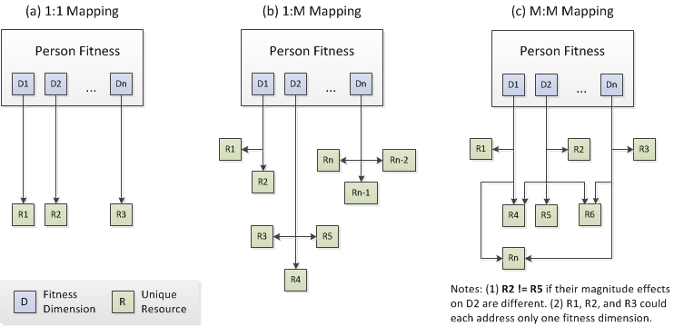
Figure 1. Mapping of Fitness Dimension Needs to Unique Resources - 2.6
- Note that we used the terms "aspect of wellbeing" and "fitness dimension" interchangeably in this paper. In this study, a fitness dimension varied from 0 to 0.99 and was subject to random decay per tick, similar to fitness decay found in evolutionary based models (Nowak and Sigmund 1998; Saqalli et al 2010). A person agent had to offset such decay by consuming resources periodically, whereby a resource could improve one or more fitness dimension. We totaled the fitness loss per person over a simulation run as
(2) where F(Di) was the current fitness value for the ith dimension, n was the total number of dimensions, and tmax was the total number of ticks in a simulation run. We then analysed the fitness loss of all persons grouped by the decision engine used, in order to compare the potential impact of information systems in different scenarios.
Configurability of Resource Diversity
- 2.7
- In a socioeconomic development context, it is important to be able to model the impact of proposed systems in scenarios that have different levels of resource diversity. This capability would permit a modeler to test systems on populations in low-resource settings versus another where market resources are more accessible and diverse. However, if a 1:1 mapping between fitness dimension and resource was used (Figure 1a), adjusting resource diversity would mean a corresponding change in the number of fitness dimensions. Using a 1:M mapping of fitness to resources (Figure 1b), we could adjust the diversity of available resources in the market while maintaining a fixed number of fitness dimensions in a person.
- 2.8
- We eventually refined our design in two ways. Firstly, we allowed a resource to potentially address more than one fitness dimension. This refinement resulted in a many-to-many (M:M) relation between fitness dimension and resources (Figure 1c). Secondly, for each dimension that a resource could address, we allowed a range of magnitudes for the potential effect. This approach led to the notion of multidimensional resources. A unique resource, Runique, was identified by the specific fitness dimensions that it could address and the magnitude effect, VDi, it had on the ith dimension that it addressed per unit quantity.
Runique = [ VD0, VD1, VD2, … , VDn ] (3) Note that a resource was produced and consumed by quantity, so the vector of values in (3) had to be multiplied by a scalar in order to get the actual effect of a consumed resource on each fitness dimension.
- 2.9
- To give a concrete example of real-world resources that may be abstracted in this way, imagine a person with needs in two fitness dimensions. For example, hunger and loneliness may be thought of as a deficiency in the fitness dimensions of physical and social wellbeing, respectively. A pizza (Resource A) may address only the physical dimension and might be sufficient for a person who is just hungry. In contrast, a hungry and lonely person would likely prefer eating out to address needs in both physical and social dimensions. A meal at a quiet café (Resource B) may be modeled as having a lower impact to social wellbeing than a meal at a bustling restaurant (Resource C). These two resources would have different magnitude values for the fitness dimension that corresponds to social wellbeing and either resource might be preferred over another depending on a person's current level of loneliness.
- 2.10
- Rows 3 - 6 in Table 1 illustrate varying 'payoffs' that a decision engine has to consider for every consumption event. Since each combination of a unique resource and consumption quantity would have led to varying effects on a person's wellbeing, there were dynamically varying utility payoffs from resource consumption depending on a person's current state of wellbeing.
Table 1: Example Calculations of Resource Consumption Effect to Multidimensional Fitness Resource A, ID# 05, to vector notation 05 → [ 0 5 ], where 1st dimension = physical wellbeing, 2nd = social wellbeing Multiply by quantity 2 units * [ 0 5 ] = [ 0 10 ] will be added to fitness upon consumption Compare consumption effect of
2 units of Resource A[ 60 80 ] + 2 * [ 0 5 ] = [ 60 90 ] Compare consumption effect of
2 units of Resource B (ID# 59)[ 60 80 ] + 2 * [ 5 9 ] = [ 70 98 ] Compare consumption effect of
2 units of Resource C (ID# 99)[ 60 80 ] + 2 * [ 9 9 ] = [ 78 98 ] Compare consumption effect of
3 units of Resource C (ID# 99)[ 60 80 ] + 3 * [ 9 9 ] = [ 87 99 ] + waste
(Note: consumption that causes > 99% fitness leads to waste)Resource Preference Person should consume 2 units of Resource C, or ID=99, since it addresses the most pressing fitness needs without causing waste - 2.11
- There is some similarity between a four-dimensional resource concept and an alternative approach of aggregating the one-dimensional effects of four resources into one overall impact measure. However, a multi-dimensional resource in Flora is a unique entity with its own lifecycle, which is clearly different from aggregating one-dimensional resources that have separate lifecycles. For example, the two-resource Sugarscape model of sugar and spice may be conceived as addressing a two-dimensional fitness measure, but those resources have distinct lifecycles (Epstein & Axtell 1996). A more appropriate comparison would be to think of multidimensional resources as a means for modeling degeneracy (Whitacre & Bender 2010).
Composability
- 2.12
- The M:M mapping of multidimensional fitness and resources increased the complexity of modeling strategies. In addition to resource consumption, our simulations included activities such as production and cleaning that were affected by a person's changing fitness levels and market information. Because of the potential resource diversity and implications to trade choice, we also wanted to model the ability of agents to specialize in market activities such as producing particular resources, cleaning waste in certain locations, or transferring resources between locations.
- 2.13
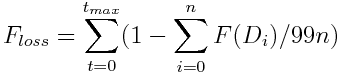
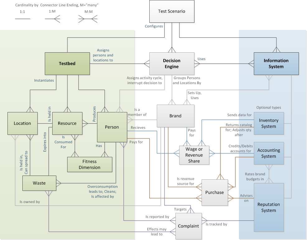
- A systematic approach was required to facilitate modeling such complex concerns. Based on the architectural frameworks of the Web (Berners-Lee 2000) and macroscope components (Borner 2011), we were inspired to group closely related modeling entities and separate those groups into orthogonal concerns. The population, location, and resource properties and dynamics were grouped into one module, which we call the testbed. To facilitate composability of different systems on top of a stable testbed, we also created separate modules for decision engines and information systems. We call this approach to modularization the TDI conceptual framework (Figure 2; Appendix 5).
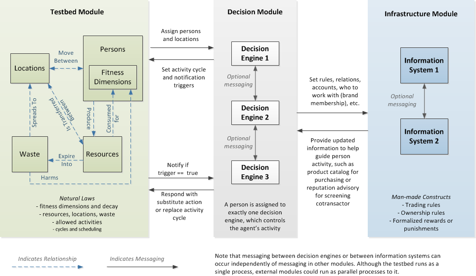
Figure 2. Overview of the TDI Framework - 2.14
- To enforce modularization, we used a message passing approach between modules. Flora specified testbed message formats from and to a decision engine. The messaging between decision engines and information systems was independent of the testbed interface, which encouraged the orthogonal development of separate modules. Although we used HTTP-accessible decision engines in earlier versions of the testbed, we switched to built-in modules to improve simulation efficiency.
- 2.15
- To lessen the amount of messaging between the testbed and a decision engine, we enforced the concept of an interruptable activity cycle. An agent typically perfomed an assigned, recurring sequence of activities for a given period of ticks. The testbed only queried a decision engine when an interrupt request was triggered by low fitness levels or when a prespecified production or consumption pattern was not possible given the current state of an agent. An effective decision strategy may be described as one that assigned activity cycles that were rarely interrupted by notification triggers.
Related Work
- 3.1
- The simulation framework in Saqalli et al (2010), which used the Cormas agent simulation software, resembles our approach. In particular, their agro-ecological and socioeconomic modules respectively correspond to the testbed and infrastructure modules in the TDI framework (Figure 1). Among the obvious differences is that, unlike the TDI framework, their approach did not specify separate modules for decision engines.
- 3.2
- A more important difference between the two frameworks lies in the modeling detail of the testbed. Flora's resources are highly abstracted and are not directly mapped to actual ecological entities and processes. It may thus be argued that the approach in Saqalli et al (2010) affords more realism than our approach. It should be noted that at the initial development stages of Flora, we planned to create a metadata library for observable resources and products with detailed lifecycle properties and numeric mapping of effects to fitness dimensions. However, as soon as resources were abstracted into numeric representations, the idea of abstracting resource lifecycles soon followed. Flora's realism is thus predicated on the ability to factor many more abstract resources and lifecycles in a simulation versus the alternative approach of using less diverse but empirically based resource entities. For large scale market-oriented applications, we believe Flora provides more realism in terms of the range of resources considered in the model and the M:M mapping between fitness dimensions and resources. Our current approach does not preclude a future adoption of empirically-based resource definition libraries.
- 3.3
- For evolutionary agent-based models that involve fitness measures, we have an example in the evolution of indirect reciprocity (Nowak & Sigmund 1996). Flora is more complex in that there is resource production, consumption, and waste cleaning. Our approach did not involve evolutionary modeling and generational inheritance. Instead, we considered the wellbeing of a semi-static population to be more appropriate for market modeling. It is important to highlight, however, the concept of "image scores" in Nowak & Sigmund (1998) as it relates to reputation systems and the infrastructure module in our modeling framework.
- 3.4
- The modular approach in Ishinishi & Namatame (1999) bears some resemblance to our modeling framework. Their Market Server module provides similar functionalities as those intended for the infrastructure module, while the Market Client is analogous to the decision module. However, (a) their modeling framework does not include a fitness-based module such as Flora where fitness decay drives agent activity, (b) they do not use the concept of activity cycles, and (c) they use real humans in gaming simulations whereas our simulation runs are currently limited to artificial agents.
Modeling of Test Scenarios
-
General Description
- 4.1
- A testbed scenario included a population of person agents who lived in a one-dimensional loop of locations. Resources were produced and consumed, where consumption counteracted the effect of fitness decay. Unused, expired resources were converted to waste that could either degrade in place or spread to other locations. A person's fitness level, as well as waste that may be collocated with that person, had an impact on the efficiency of production, consumption, or cleaning activity.
- 4.2
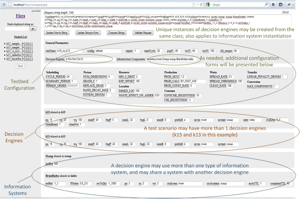
- To instantiate a test scenario, the modeler specified the numbers of persons, locations, and resources to simulate in the run (Appendix 2). Configuration settings were changed from default testbed parameter values as needed. A modeler added at least one decision engine, which may require its own separate set of configuration settings. If a decision engine required an information system, the user interface automatically produced the required form to properly instantiate and configure the required system. See Appendix 4 for links to sample run requests.
- 4.3
- Prior to the beginning of the simulation run, each person was assigned a decision engine. The decision engine created an activity cycle for each person and performed optional information system setup such as membership or reputation system accounts. For each tick in a simulation run, the update schedule randomized the order in which each person acted. The testbed normally performed a recurring activity as specified by a person's activity cycle. If the person had a notification trigger on, the testbed instead quered the person's decision engine for a potential substitute activity to perform.
- 4.4
- Flora generated a report at the desired frequency during simulation runs, including accumulative fitness loss per person as the simulation progressed. Instantiated decision engines and information systems were also queried for periodic reports. The modeler was expected to be aware of all available reported results for a given test scenario and to preprocess the generated data as necessary. Examples of real-time and post-run visualizations are shown in Appendix 3.
- 4.5
- For more details, see Appendix 1 which outlines entity properties, configuration options, and restrictions. The pseudo-code listing in the appendix provides a logical overview of the simulation process, including the message formats for production and consumption activities.
Runs
- 4.6
- The testbed design intent was evaluated in a series of test scenarios, with at least 24 repeat simulation runs performed for each test and each run lasting at least 30 cycles. The tests evaluated the population effects of using different information infrastructure components starting from a simple scenario involving an inventory system without accounting or reputation systems. Infrastructure components were then used in combination with those used in previous scenarios to model progressively sophisticated populations. A decision engine template was used to change the infrastructure scenario.
- 4.7
- The parameter values from each run were saved with the simulation results for population fitness metrics. Datasets from different run iterations were combined to form CSV files which were then imported to a statistical analysis application (STATA). Three of the summary metrics used were aliveNum and effCycle, which were calculated as follows:
- aliveNum: The number of persons using the same decision engine who have fitness dimension values all > 0. If any of the fitness dimensions was < 1, a person was considered dead.
- effCycles: This metric was analogous to disability adjusted life years (DALY) (Murray 1994), but without the concept of disease or health burdens. Instead, effCycles was a measure of the wellness of a person in all dimensions after taking into account needs that have not been addressed through resource consumption. The effective lived cycles was calculated as:
- effCycles = 100% * (MAX_CYCLE - cycles_lost) / MAX_CYCLES,
- cycles_lost for dead agents = [(MAX_CYCLE*ticks/cycle) - tick_of_death]
- cycles_lost for living agents = [(400 - sum of fitness dimensions)/400])
- trackedLoss: this was the cumulative cycles_lost per person for each simulation run, which complemented the metric of effCycles
- 4.8
- The standard configuration settings for all tests, unless varied under specific test scenarios, were:
- maxCycle: 30 cycles per run
- CYCLE_PERIOD: 24 ticks per period
- Number of person (popN): 48
- Number of locations (locN): 64
- Number of brands (numBrands): 16
- Number of members (numP) per brand: 3
- Number of locations (numlocs) per brand: 4
- 4.9
- The randomized variables in this study were:
- Starting values for each fitness dimension per person
- Fitness decay: 1 - 3 loss per tick, independently randomized per dimension per person
- The resource that was assigned for production in each location
- The order of resources as presented in the catalog when the inventory system was queried for available resources
- 4.10
- The analysis used parametric and non-parametric methods, abbreviated as the following in the presentation of results:
- ttest: Student's T-test; mean comparison test
- ksmirnov: Kolmogorov-Smirnov equality of distributions test
- ranksum: Wilcoxon rank-sum test; equality tests on unmatched data
- median: non-parametric equality of medians test
Results and Discussion
- 5.1
- We tested the effect of having different infrastructure components on population fitness loss. Starting with a scenario of using only an inventory system, we added an accounting system and then a reputation system to model increasingly complex sociotechnical infrastructures. For each infrastructure scenario, we investigated the effect of varying the values of specific parameters, changing one parameter value for each test scenario. Each test scenario was then repeated multiple times as explained in the Methods section.
- 5.2
- Before presenting our results, it is important to emphasize that our simulation tests were meant to demonstrate our conceptual approach to modeling and how Flora addressed our testbed design requirements. This paper is similar to Nongaillard & Mathieu (2011) in that we were not attempting to provide solutions to specific research problems or explanations for empirical social observations. In-depth exploration of each test scenario was considered out of scope and purposely excluded in favor of demonstrating the breadth of method applicability.
Test Scenarios with Inventory System Only
- 5.3
- Decision engine "k12" was configured without an accounting or reputation system. The inventory system provided a view of available resources for consumption,
Ravailable = { RL0, RL1, …, RLn }, (4) where RLn was the resource and quantity held in Location ID=n at the time the view was requested and where quantity > 0. Unless configured otherwise, it was possible for more than one location to hold the same resource, so the number of unique resources was not necessarily equal to the number of locations. Each person was allowed to remove resources from a location without needing to purchase.
- 5.4
- Figure 3 shows the effect of different levels of resource diversity, Rdiversity, on population fitness.
Rdiversity = number of resources with unique IDs (5) where uniqueness was defined in (3).
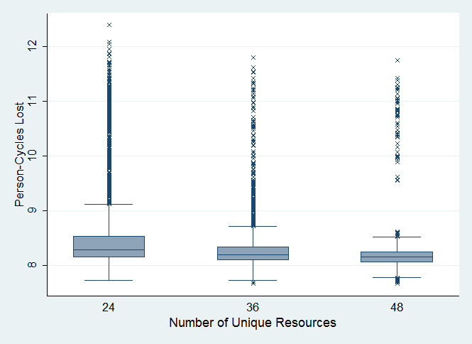
Difference in fitness loss, 24 vs. 36 unique resource IDs:
ttest: P < 0.0000, t = 16.12 (mean loss:8.62 vs. 8.29)
ksmirnov: P = 0.000, D = 0.1758
ranksum: Pr = 0.0000, z = 14.341
median: Pr = 0.000, χ2 = ~135.34Difference in fitness loss, 36 vs. 48 unique resource IDs:
ttest: P < 0.0000, t = 8.5885 (mean loss: 8.29 vs. 8.19)
ksmirnov: P = 0.000, D = 0.1829
ranksum: Prob. = 0.0000, z = 11.339
median: Prob. = 0.000, χ2 = 54.6133
Figure 3. Effect of Resource Diversity Interpretation 1: Higher levels of resource diversity led to better population fitness.
- 5.5
- The results summarized in Figure 3 aligned with our intuition that with more diverse resources, a person would be able to choose a resource that fits specific needs in a consumption activity. Limited product choices led to less optimal consumption patterns. It is also important to note that the decrease in fitness loss was smaller when the diversity range being compared was on the higher range. In other words, there was marginally decreasing benefit to having additional resource diversity.
- 5.6
- Figure 4 shows the effect of varying the maximum number of fitness dimensions that a resource can address, DmaxAddressableByResource:
DmaxAddressableByResource = NUM_DIMENSIONS - MIN_0_DIGITS (6) where the NUM_DIMENSIONS was a person's number of fitness dimensions as defined in (1) and MIN_0_DIGIT was the minimum number of zero values that a resource must have and must be less than NUM_DIMENSIONS. This scenario simulated the intuition that no single product could address all fitness dimensions. We set NUM_DIMENSIONS to 4 and varied MIN_0_DIGITS from 1 to 3. No accounting or reputation system was used in this test scenario.
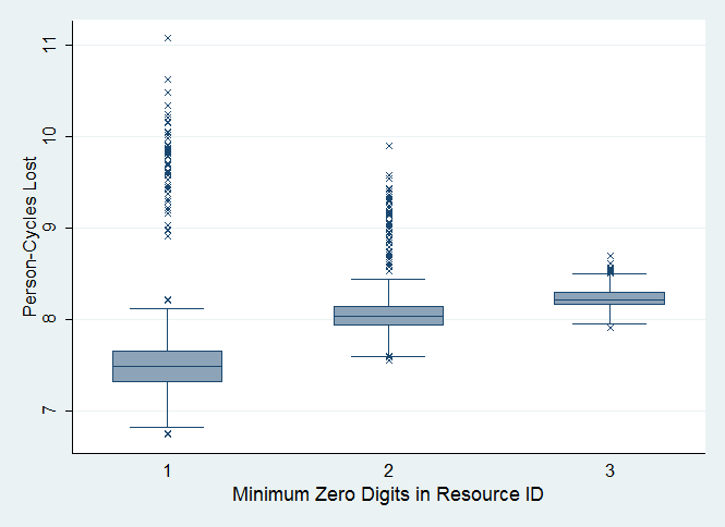
NOTE: The maximum number of fitness dimensions addressed by a resource decreased for every unit of increase in MIN_0_DIGITS. Difference in fitness loss, minimum 1 vs. 2 zero digits:
ttest: P < 0.0000, t = -29.39 (mean loss: 7.57 vs. 8.07)
ksmirnov: P = 0.000, D = 0.8099
ranksum: Pr = 0.0000, z = -36.099
median: Pr = 0.000, χ2 = ~1400Difference in fitness loss, minimum 2 vs. 3 zero digits:
ttest: P < 0.0000, t = -18.89 (mean loss: 8.07 vs. 8.23)
ksmirnov: P = 0.000, D = 0.5512
ranksum: Prob. = 0.0000, z = -26.730
median: Prob. = 0.000, χ2 = 616.7
Figure 4. Effect of Different MIN_0_DIGITS Interpretation 2: Having resources that could target specific fitness dimension needs led to more fitness loss but less variance in the observed values.
- 5.7
- The results in Figure 4 presented an unexpected twist to our initial expectations. The results indicated that increasing the number of fitness dimensions that a resource could address led to less fitness loss, since it enabled a person to potentially address more than one fitness need in one consumption event. However, there was more variance in the population fitness when the resources were restricted to addressing less number of fitness dimensions. This somewhat surprising result was likely due to the greater likelihood of targeting specific fitness needs when there were more zero-digits in the resource ID. Each consumption activity effectively addressed the most pressing need, but at the same time, there was less likelihood of addressing other fitness dimension needs and so the overall fitness loss was greater than when resource IDs were allowed to have less zero-digits.
- 5.8
- Figure 5 shows the effect of hoarders on population fitness. We simulated hoarders, {Hi → n}, as agents who asked to view all available resources, Ravailable in (4), from all brands even if they did not share in the production activities of other brands. In contrast, non-hoarders asked to view only items that have been produced within their brands. This effectively gave hoarders more options when shopping for resources to consume. Since no purchase was necessary in the absence of an accounting system, a person simply removed the preferred resource as needed. Note that hoarding in this sense did not necessarily imply the accumulation of resources, but instead hoarders hid resources and thus avoided sharing with non-hoarders.
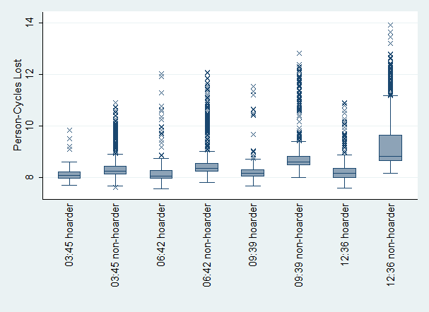
Difference in fitness of hoarders in 3:45 versus 12:36 tests
ttest: P < 0.0218, t = -2.30 (mean loss: 8.16 vs. 8.35)
ksmirnov: P = 0.045, D = 0.1736
ranksum: Prob. = 0.1063, z = -1.615
median: Prob. = 0.087, χ2 = 2.9340Difference in fitness of non-hoarders in 3:45 versus 12:36 tests
ttest: P < 0.0000, t = -25.34 (mean loss: 8.38 vs. 9.33)
ksmirnov: P = 0.000, D = 0.6956
ranksum: Prob. = 0.0000, z = -29.360
median: Prob. = 0.000, χ2 = 888.3521
Figure 5. Effect of Different Ratios of Hoarders to Non-hoarders Interpretation 3: (a) More hoarders led to worse population fitness for non-hoarders, and (b) hoarders had less fitness loss than non-hoarders.
- 5.9
- The results in Figure 5 aligned with our intuition that a hoarding population subset would be healthier since they would have had access to a more diverse resource set, compared to non-hoarders who were not aware of the hoarded resources and therefore could not have accessed them. A higher ratio of hoarders to non-hoarders led to more fitness loss by non-hoarders. It is also worth stating that the fitness loss by hoarders was not as affected by the ratio of hoarder to non-hoarders.
Test Scenarios with Inventory and Accounting Systems
- 5.10
- The effects of hoarders on non-hoarder fitness can be minimized through the use of currency or accounting systems to limit resource access and encourage fairer means of resource distribution. Our conception of currency was primarily related to community currencies, barter tracking systems, or other decentralized currency systems that have been designed as a complement or alternative to centrally issued currencies at the national level (Schroeder et al 2011). However, to simplify our simulation of two decentralized currency system scenarios, we purposely avoided modeling administrative protocols and instead focused on modeling only the essential accounting system features. We refer to these highly-simplified models of currency systems as, simply, accounting systems.
- 5.11
- For the following test scenarios, decision engine "k13" was configured to use an accounting system, but not a reputation system. A purchase was required to obtain a location-specific claim key, which could then be used to remove resource equal to the purchased quantity. There were two type of accounting systems tested, one simulating a local exchange trade system or LETS (Linton 1996) and another simulating entity-issued currency brands or OCAUP (Sioson 2009). In both systems we set an initial account balance for each added brand member (Table 2). We modeled LETS credits as issued-once tokens that circulated among users of the same currency, while OCAUP currency were modeled as cyclically-issued expense and revenue budgets that were periodically decreased whenever a buyer's credits cancel seller debits.
Table 2: Comparison of LETS and OCAUP Accounting Accounting Event LETS Accounting OCAUP Accounting Setup of accounts All account balances = 0 All account balances = 0 Effect of a member joining brand where initBal = Initial balance per member revenueAcct - initBal
memberAcct + initBalrevenueAcct - initBal
memberAcct + initBalEffect of Purchase where amt = payment amount buyerAcct - amt, (buyer)
revenueAcct + amt, (seller)buyerAcct - amt, (buyer)
revenueAcct + amt, (seller)Calculation of Wages, W, or Revenue Distribution, revDist, where numP = number of brand members revDist per member =
(revenueAcct - numP*initBal) / numPW per member =
itemPrice*addedQty /numPNotes InitBal was considered as currency that were reused and circulated based on transaction activity. This model led to a constant number of circulated tokens throughout a simulation run. The amount of currency that could be used for payment dynamically changes throughout the run, since credits and debits were regularly co-created when paying wages and co-cancelled when a purchase was made. - 5.12
- Figure 6 shows the effect of having different numbers of trading brands, numB, on population fitness, by the type of accounting system used. The total number of people and locations were held constant at 48 and 64, respectively, so that membership per brand, numP, and inventory items per brand, numR, increased as the numB decreased. No reputation system was used in these test scenarios.
numP = 48 / numB (7) numR = 64 / numB (8) 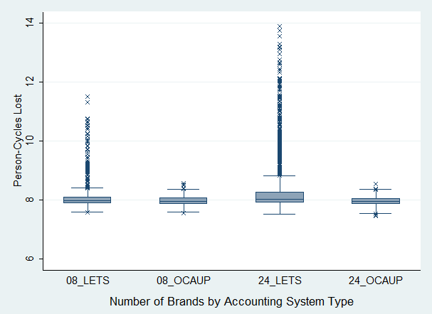
Difference in LETS user fitness based on 8 vs. 24 trading brands scenarios:
ttest: P < 0.0000, t = -11.52 (mean loss: 8.08 vs. 8.46)
ksmirnov: P = 0.000, D = 0.1645
ranksum: Prob. = 0.0000, z = -5.616
median: Prob. = 0.001, χ2 = 11.4345Difference in OCAUP user fitness based on 8 vs. 24 trading brands scenarios:
ttest: P < 0.0442, t = 2.0129 (mean loss: 7.97 vs. 7.96)
ksmirnov: P = 0.324, D = 0.0391
ranksum: Prob. = 0.1665, z = -1.384
median: Prob. = 0.479, χ2 = 0.5017
Figure 6. Effect of Number of Brands Interpretation 4: LETS users, compared to OCAUP users, were more likely to experience greater fitness loss as the number of trading brands (numB) increase, which in a constant population implied decreases in both the numbers of members (numP) and resources (numR) produced per brand.
- 5.13
- The results in Figure 6 aligned with our intuition that LETS members were better off belonging to brands with larger membership and/or number of resources produced. This result can be explained by a larger brand having more revenue to distribute to its members on a periodic basis, so that members would have had more regular income. Smaller brands were more prone to erratic revenue patterns.
- 5.14
- Figure 7 shows the effect of different initial account balances by the type of accounting system used. In a LETS system, each person that joined a participating brand was assigned a debit limit, initBal, which was modeled as a starting balance of issued tokens. A LETS accounting system restricted the number of tokens that circulated within a participating community.
- 5.15
- In an OCAUP system, currency was periodically issued by each brand independently according to the quantity of resource produced by each brand member. In the highly simplified test scenario, members were issued credits as wages while the brand accrued the corresponding debits in its revenue budget. A purchase resulted in the equivalent cancellation of buyer credits and seller debits. The dynamically changing budgets encouraged cyclical currency issuance by brand, with the amount of periodic budget increases varying according to each brand's market performance. No reputation system was used in these test scenarios.
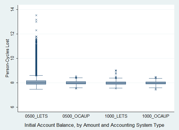
Difference in LETS user fitness based on 500 vs. 1000 initial balance:
ttest: P < 0.0000, t = 12.2651 (mean loss: 8.27 vs. 7.98)
ksmirnov: P = 0.000, D = 0.1658
ranksum: Prob. = 0.0000, z = 5.544
median: Prob. = 0.001, χ2 = 10.3138Difference in OCAUP user fitness based on 500 vs. 1000 initial balance:
ttest: P < 0.0210, t = 2.3098 (mean loss: 7.99 vs. 7.97)
ksmirnov: P = 0.034, D = 0.0575
ranksum: Prob. = 0.0301, z = 2.168
median: Prob. = 0.079, χ2 = 3.0866
Figure 7. Effect of Amount of Initial Account Balance Interpretation 5: LETS users, compared to OCAUP users, were more likely to experience greater fitness loss as the initial account balance decreases.
- 5.16
- The results in Figure 7 aligned with our intuition that the higher the starting balance, the more LETS tokens there were that could circulate in a market and therefore the more chances for a brand to earn revenue to distribute to its members. Unlike our simulated model of the LETS accounting system, a brand in an OCAUP system was not restricted by its revenue stream or the total of initial account balance in being able to issue wages to its members. An OCAUP brand was thus able to provide a regular income source to its members regardless of the amount of circulated tokens, which in LETS was ultimately dependent on initial account balance if the number of users was held constant.
- 5.17
- It is important to note that the results in Figure 6 and 7 were gathered using highly simplified models of accounting systems that assigned fixed product prices and lacked administrative protocols.
Test Scenarios with Inventory, Accounting, and Reputation Systems
- 5.18
- While accounting systems might encourage fairer means of resource distribution according to resource contribution, it was not immediately clear whether they could effectively deter polluters and other detrimental socio-economic behavior. Reputation systems help extend the concept of equitable distribution by helping tie observed socioeconomic behavior to specific market identities or brands. Disreputable brands may then be targeted for economic non-cooperation, such as through purchase avoidance.
- 5.19
- If market participants care about their reputations, then noncooperation could potentially influence malevolent agents to change behavior. We assumed that the potential level of cumulative influence would be greater if a person was likely to suffer greater fitness loss (Equation 2) due to economic noncooperation. Under this assumption, we considered a reputation system to be effective if the type of noncooperation that it encouraged led to a clear difference between the fitness losses of good and malevolent agents. This difference in fitness loss was more easily observed if the malevolent agents did not revise strategies such as changes to activity cycles or brand membership. Therefore, we used almost identical, non-adaptive decision engine strategies in the following test scenarios.
- 5.20
- We created test scenarios of a reputation system based on accounting system and pollution related criteria. Pollution was waste from a resource quantity that had expired, had not been cleaned or degraded, and potentially had spread to other locations.
RT → WT (9) where RT was the quantity of resource that expired and became the waste or quantity of pollution WT. The resource expired when T > Rexpiration_tick,
Rexpiration_tick = Tproduction + EXP_OFFSET (10) where Tproduction was the tick value when a resource was produced and EXP_OFFSET was an integer duration in units of ticks, which was the same for all resources in the default configuration.
- 5.21
- A quantity of waste could spread to adjacent locations:
Wspread = (Wquantity*SPREAD_RATE) - SPREAD_THRESHOLD (11) where Wquantity was the quantity of waste in a location and where the other parameters were specified in the configuration of the test scenario. If the calculated Wspread was < 0, the waste was not transferred to adjacent locations. Otherwise, Wspread / 2 was transferred to locations right before and after the source location ID.
- 5.22
- Pollution was defined as any waste that affected a person fitness and that could have spread to other locations. There were two types of brands: those whose members included cleaning of waste in their activity cycles (non-polluters), and those that did not clean but concentrated on production activities instead (polluters). The latter's locations therefore accumulated waste from expired resources, which potentially affected the fitness dimensions and efficiency of producers, consumers, and cleaners. When the effect felt by an agent was greater than its preset thresholds, it reported a complaint to a reputation system.
- 5.23
- Decision engine k15 was programmed to query a reputation system during a purchase event in order to evaluate buyer or seller reputation. The reputation system periodically queried known accounting systems for updates on currency activity metrics. It also received and tallied complaints from producers, consumers, and cleaners who have had a negative effect from pollution. The reputation system settings applicable to brand evaluation were accounting-related such as net account balance, or complaint-related such as the maximum number of consumer complaints per summary period over which a brand was blacklisted. Note that the reputation system applied to groups of agents, which we call brands, and not to individual agents as modeled in Schlosser et al (2006) and Wierzbicki & Nieke (2011).
- 5.24
- In the following test scenarios, the No-Screening case had the reputation system turned off, which resulted in all purchases being automatically approved without buyer or seller screening. Buyer-Screening simulated the scenario where sellers refused to accept the currency of buyers belonging to disreputable brands, while Seller-Screening simulated the scenario where buyers refused to buy products from disreputable seller brands.
- 5.25
- Figure 8 shows the impact of a reputation system on the fitness of non-polluters. A reputation system should minimize adverse impact on non-polluters. This analysis compared the fitness loss of non-polluters in scenarios with and without reputation systems.
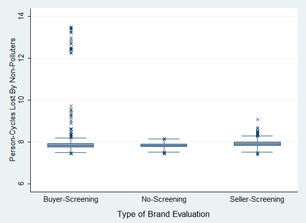
Difference in non-polluter fitness between No-Screening and Seller-Screening:
ttest: P < 0.0000, t = -18.61 (mean loss: 7.84 vs. 7.92)
ksmirnov: P = 0.000, D = 0.2310
ranksum: Prob. = 0.0000, z = -17.248
median: Prob. = 0.000, χ2 = 188.5952Difference in non-polluter fitness between No-Screening and Buyer-Screening:
ttest: P < 0.0000, t = -5.40 (mean loss: 7.83 vs. 7.90)
ksmirnov: P = 0.003, D = 0.0557
ranksum: Prob. = 0.2729, z = -1.096
median: Prob. = 0.806, χ2 = 0.0601
Figure 8. Effect of Type of Currency Brand Evaluation on Non-Polluter Fitness Interpretation 6: There was a difference, however small, in non-polluter fitness in both Buyer and Seller-Screening relative to the No-Screening case. The difference in median fitness loss for Buyer-Screening was less convincing.
- 5.26
- The results in Figure 8 show that the effects of a reputation system could be targeted towards specific subsets of the population. As a matter of design objective, a reputation system should minimize any adverse side-effects to reputable brand members to encourage their participation. For Seller-Screening by buyers, there was statistical evidence for adverse impact to reputable brand members, even if the fitness loss was only marginally higher. This difference between seller and buyer screening was likely from the design of the K15 decision engine, in which a purchase rejection by a buyer led to lost opportunity for more appropriate consumption, whereas seller rejection did not necessarily affect the consumption pattern of a seller.
- 5.27
- Figure 9 shows the impact of a reputation system on the fitness of polluters. In this test scenario, a reputations system was considered effective if its use led to greater fitness loss for polluters. This analysis compared the fitness loss of polluters in scenarios with and without reputation systems.
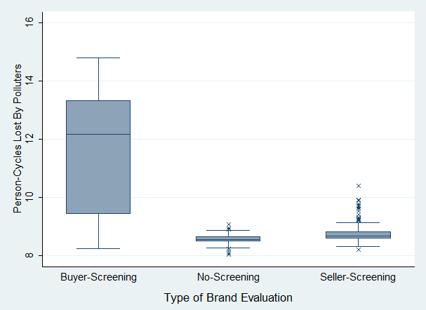
Difference in polluter fitness between No-Screening and Seller-Screening:
ttest: P < 0.0000, t = -9.94 (mean loss: 8.57 vs. 8.75)
ksmirnov: P = 0.000, D = 0.3567
ranksum: Prob. = 0.0000, z = -9.908
median: Prob. = 0.000, χ2 = 62.7267Difference in polluter fitness between No-Screening and Buyer-Screening:
ttest: P < 0.0000, t = -24.16 (mean loss: 8.6 vs. 11.5)
ksmirnov: P = 0.000, D = 0.7788
ranksum: Prob. = 0.0000, z = -16.596
median: Prob. = 0.000, χ2 = 269.4435
Figure 9. Effect of Type of Currency Brand Evaluation on Polluter Fitness - 5.28
- Figure 10 shows the relative impact of a reputation system on the difference between polluter and non-polluter fitness. In this test scenario, a reputation system was considered effective if its use led to a significant difference between non-polluter and polluter fitness. This analysis compared the fitness loss gap in scenarios with and without reputation systems.
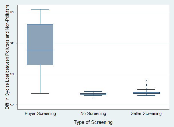
Difference in polluter-nonpolluter-fitness-loss--difference between No-Screening and Seller-Screening:
ttest: P < 0.0013, t = -3.32 (mean diff: 0.73 vs. 0.82)
ksmirnov: P = 0.013, D = 0.3000
ranksum: Prob. = 0.0033, z = -2.937
median: Prob. = 0.028, χ2 = 4.8400Difference in polluter-nonpolluter-fitness-loss-difference between No-Screening and Buyer-Screening:
ttest: P < 0.0000, t = -12.82 (mean diff: 0.73 vs. 3.63)
ksmirnov: P = 0.000, D = 0.9231
ranksum: Prob. = 0.0000, z = -8.314
median: Prob. = 0.000, χ2 = 72.5377
Figure 10. Effect of Type of Currency Brand Evaluation on the Difference between Polluter-and-Non-Polluter Fitness Interpretations 7 and 8: Buyer-Screening was much more effective than Seller-Screening as a means for applying pressure on malevolent socioeconomic participants.
- 5.29
- The results in Figures 9 and 10 show that polluters experienced much greater fitness loss in the Buyer-Screening scenario compared to Seller-Screening and relative to the No-Screening scenario. This indicated that seller rejection of disreputable brands was more effective in deterring detrimental socio-economic behavior. These results justify a preference towards enabling sellers to screen buyers as a more effective form of reputation system for applying selective pressure.
- 5.30
- Figure 11 shows the effect of cumulative brand rejections on the fitness of brand members. In this scenario, a reputation system was considered more effective if its use led to more predictable correlation between brand rejection and member fitness loss. This analysis compared the correlation between fitness loss and the number of purchase rejections caused by buyer or seller refusal to transact with disreputable brands.
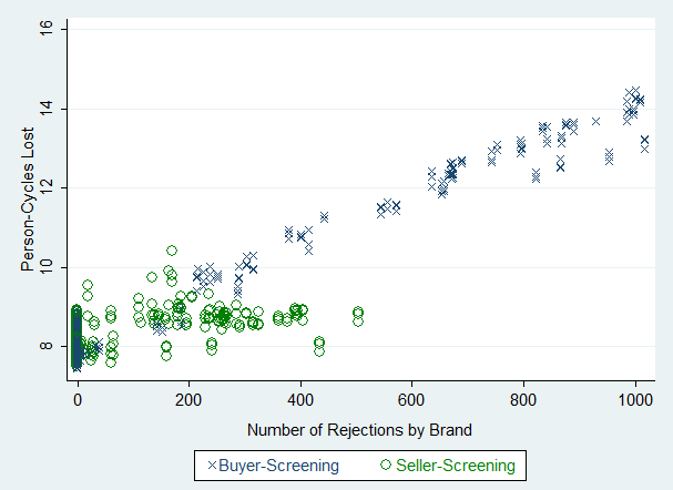
Seller-Screening Robust Regression:
Coeff. rejects_by_brand: 0.0026328
F = 1758.34, Prob > F = 0.0000, t = 41.93Buyer-Screening Robust Regression:
Coeff. rejects_by_brand: 0.0065716
F = 1.2e05, Prob > F = 0.0000, t = 343.33
Figure 11. Tracked Loss vs. Number of Brand Rejections by Type of Currency Brand Evaluation Interpretation 9: Buyer-Screening has a more predictable deterrence effect than Seller-Screening based on the observed correlations between fitness loss and the number of brand rejections.
- 5.31
- Figure 11 shows a clear correlation between the number of brand rejections and fitness loss in the scenario where sellers perform Buyer-Screening. There was less convincing correlation in the Seller-Screening scenario. When considering investments in technical infrastructures as means for socioeconomic development, these results clearly support Buyer-Screening by sellers as a more effective approach to reputation system design that results in predictable impact.
Study Limitations
- 6.1
- One of the limitations of the testbed was the uniformity in the lifecycle of resources having the same ID. It should be more realistic to introduce variability in resource lifecycles even for those having the same ID, analogous to cars having different usable lifetimes depending on manufacturer brand. This variability in lifecycles may include additional parameters or factors to use in calculating a resource's production rate, usable lifetime, waste degradation, and waste spread.
- 6.2
- While earlier versions of our testbed interfaced to decision engines via the HTTP protocol, we found that approach to be much slower than interfacing to other modules via single thread messaging. We are currently revising Flora to realize the goal of using distributed modules that interface through lower latency communication protocols such as TCP or UDP. It is also worth noting that the network delay has less pronounced impact if multiple simulation runs are parallelized through different process threads or servers.
- 6.3
- Other limitations in our study were related to the lack of learning capability or adaptive behavior in the decision engines, or paucity of features in the infrastructure components that could have improved decision making. Ideally, decision engines will change production, consumption, and cleaning activities to lessen the fitness loss of an individual. Our current implementation primarily affected consumption patterns, with the activity cycle remaining more or less the same throughout a run even with cycle interrupts. In addition, our models of accounting systems did not include administrative protocols and only assigned fixed product prices. Future studies should factor price competition to afford more realism in the simulations.
- 6.4
- The limited learning in decision engines, combined with the testbed feature of replacing dead persons with 'fresh incarnations', led to non-normal distributions of fitness loss in the population. In particular, there was a long tail representing a few people who experienced large fitness loss relative to the majority of the population. It was likely that the replacement feature introduced baseline undulations in the distribution tail. Decision engines with more intelligent adaptations during a run should lead to a more normal distribution.
- 6.5
- Another feature that could lead to more normal distributions of fitness loss is to enable varied individual response to consuming a particular resource. We could also dynamically alter individual preferences on which accounting metrics and reputation scores to use. Our study enforced the same thresholds for triggering brand rejection throughout the population, whereas a more realistic scenario would allow a range of reputation thresholds at which individual or organizations would reject another brand.
- 6.6
- The numbers of persons, locations, and resources were intentionally kept under 100 to simplify the demonstration of the method. In-depth modeling and studies of complex sociotechnical phenomena would require much greater numbers of these testbed objects. Each test scenario was also limited to testing the use of one decision at a time, even though Flora is easily configured to allow the simultaneous use of different test engines. This limitation was intended to simplify the analysis, with the primary goal of generating testbed expectations and rules of thumb that could be applied to future test scenarios.
Conclusion
- 7.1
- We have demonstrated the use of Flora as a testbed within the TDI framework, using a M:M mapping of fitness dimensions to resources. We applied our method to test several hypotheses related to the impact of various information infrastructure components including inventory, accounting, and reputation systems. We found that increased diversity in resources, as well as having resources that could target specific fitness needs, led to better population fitness. Accounting systems that allowed organizations to issue currency independently as budgets were more robust in terms of minimizing fitness loss, compared to systems that limited an organization or community's ability to issue decentralized currency. We also found screening buyers to be more effective than screening sellers as a means for deterring detrimental socioeconomic behavior. We hope to farther qualify these findings through in-depth studies of specific cases and under more varied test scenarios.
Appendix 1: Modeling Details
- 8.1
- The project homepage is at http://edgarsioson.com/flora/. We implemented the model directly in the PHP language (http://php.net/) using an object-oriented programming approach. The source code is maintained in https://bitbucket.org/siosonel/flora using the Mercurial version control system (http://mercurial.selenic.com/). In the project homepage, example visualizations are given for test scenarios with and without reputation systems.
- 8.2
- Below are model entity descriptions, scheduling approach, and pseudocode listings.
Person
- ID: integer > -1
- fitness dimensions
- default of four dimensions, [F_1, F_2, F_3, F_4 ], each with a randomly assigned initial value between 60 - 90%; number of dimensions was configurable
- 0 - 99%; person was dead if any fitness dimension < 1; cannot exceed 99%
- this was subject to a fixed or randomized decay rate per clock tick.
- holding: resources that a person could have consumed or put in a location, grouped by expiration tick
- activity cycle: repeating activity pattern within a globally specified number of ticks, subject to interrupt requests based on a decision engine's reply to notification trigger
- decisionURL: when a notification trigger was true during a cycle, the testbed queried the decisionURL for interrupt request
- triggers:
- minF: contact a decisionURL when a fitness dimension fell below this threshold
- maxF: contact a decisionURL when the fitness dimension with the lowest value rose above this value
- holdingNum: contact a decisionURL when number of held resources fell below this threshold
- (auto): contact decisionURL when it was not possible to perform an activity per an assigned recurring pattern
- experience: quantity of resource produced by person, listed by quantity. Production rates may be improved by previous experience with the same resource
- loc: person's current location
- keys: to add or remove resource quantities from a location where a person was not already specified as an adder or remover by person ID
Resource
- ID:
- exactly four digits were used in this paper, but adjustable by run
- was configurable to include a minimum number of zero digits to represent the observation that no single resource could possibly address all fitness dimensions
- see Table 2 for example calculations of multidimensional effect
- qty: quantity of the resource when it was instantiated
- expiration: calculated as current tick + EXP_CONST + sum of all id-digit values; all resource held past the expiration tick was converted to waste
- production rate:
- BY_DIGIT_SUM: calculate production rate as 40 - sum of all id-digit values
- BY_DIGIT_AVE (default): calculate production rate as 10 - (sum of all digit values/4)
- BY_CONSTANT: set production rate manually
Location
- ID: integer > -1
- resource: the resource held in the location; only one resource ID was held in a location at any given time
- quantity: the quantity of the held resource
- waste: quantity of any remaining resource that had been converted to waste and had not been cleaned or degraded
- keys: Flora allowed ownership, adding, removing, or viewing change requests for a location based on pre-specified person ID or matching claim keys
- history: this was analogous to person history. Production history for a certain product could increase the corresponding production rate. A location with accumulated history, and thus efficiency, for producing a certain resource was analogous to tradable capital.
- Applicable configuration options: IMMED_LOC, the maximum distance that was accessible to a person within one tick.
Scheduling
The simulation ran asynchronously, with an option to interrupt based on notification triggers. The possible configuration settings were:
- CYCLE_PERIOD: number ticks in a cycle before an activity pattern repeats
- CYCLE_BUFFER: the number-of-ticks-window wherein a given activity may occur within the previous cycle in order to be considered relevant to a calculation within the current cycle. For example, producing resource 1111 on tick=10 every cycle will add a bonus to production efficiency. With a cycle buffer of 2, it would not matter if the 1111-production occurred on tick = 8, 9, 10, 11, or 12 of the previous cycle.
- SUMMARY_PERIOD: when a summary period is reached, fitness metrics are summarized by decisionURL, with the collected data to be saved to disk at the end of the run
- maxCycle: how many activity cycles recurred in a run
- PERSON_ORDER:
- RANDOM: (default in later code revisions) randomize person order every cycle
- TOFRO: (applicable to earlier code revisions) randomize where to start the cycle in the person queue and whether to process person id's in increasing or decreasing order with loop back; this is not completely random in that the same person order will be followed given a starting person and direction.
- STATIC: (applicable to earlier code revisions) use same person order every cycle except to prioritize interrupt requests; list of person id's in the interrupt request queue is randomized every cycle
Pseudo-Code
The following listings illustrate the high-level testbed logic.
*************************************************************
Listing 1: Main Routine
*************************************************************

Instantiate optional infrastructure objects: inventory, accounting, and/or reputation systems

Instantiate popN Persons with each fitness dimension randomized between 60 - 90%
Instantiate locN Locations
Instantiate Decision Engines to be tested:

Foreach decision engine:
    Assign brands, locations, and members
    Assign address of instantiated infrastructure objects

Foreach person:
    Assign the applicable decision engine based on brand membership
    Query Person->decisionURL for cycle, F_min, F_max

while (cycleNum < MAX_CYCLE):
    shuffle(person_order); //default random order as used in this paper

    foreach person_id:
        recalculate Person->fitness due to decay

        if notification_trigger == true:
            act_i = query person's decisionURL for interrupt request

        if (act_i) perform act_i
        else perform act specified by person's activity cycle

        person->lastTick = currTick

        if (cycleNum == summaryPeriod):
            calculate summary metrics
            save summary report to disk

end while
exit

*******************************************************************
Listing 2: Sample decision engine logic (separate module from testbed)
*******************************************************************

If initial_setup:
    Reply with cycle, one predefined activity for each tick in a cycle period

Else:
    If Person->Fmin < 50:
        Check holdings and query inventory system for all locations with resources available for consumption
        Calculate which resource and quantity results in highest fitness average without causing waste //see examples in Table 1
        Purchase as needed if person is not preauthorized as a remover for location:
        Query the accounting system to see how much resource the person could afford;
        Query the reputation system to screen the seller or buyer
        Reject the purchase if the seller or buyer is disreputable

    Else if Person->F > Fmax:
        Instead of consuming, take the opportunity to transfer resources between locations,
        or move to another location to get resources that would increase the degeneracy level of held resources

     ********************************************************************
Activities
The following activities were allowed in Flora. Exactly one activity was required per person per cycle tick.
- Production
- Message format: '{"act": ["P", resource_id, quantity (, location_id)]}'
- Production Rate: The method for calculating production rates is configurable and was described as a Resource parameter. This quantity was used as an upper limit to produced quantity. It may be desirable to limit production quantity in order to limit the quantity of expired resources turning into waste.
- If location ID was specified and the person had appropriate authorization, the resource was held in the location and the quantity added towards the location's history; otherwise, the resource was added to the person's holding
- To simulate the notion of labor specialization, a person's accumulated experience in producing a particular resource had a logarithmic relation to production efficiency. In addition, a person who maintained a routine schedule, e.g., producing the same resource on the same tick in recurring cycles, received a nominal added production gain. These potential variations in task performance across a population were attempts to relativize activity payoffs against emergent individual properties and experiences, instead of against a globally assigned payoff matrix that remained static throughout a run.
- Consumption
- format: '{"act": ["C", resource_id, quantity (, location_id)]}'
- The quantity was used as an upper limit to the consumption quantity. The quantity could be reduced all the way to zero if the quantity held by the person or applicable location was less than specified.
- If location ID was specified and the person had appropriate authorization, the resource was removed from the location; otherwise, the resource was removed from the person's holding
- Clean
- format: '{"act": ["W", "", quantity (, location_id)]}'
- The quantity was used as an upper limit to cleaned quantity by person, but superseded by configuration if CLEAN_RATE was less than activity quantity.
- If location ID was specified and the person had a matching key for that location, the resource used for cleaning was removed from the location; otherwise, the resource was removed from the person's holding
Convert and transfer activities were not used in this study, but will be developed in later versions of Flora.
Messaging between Entities and Modules
We used a message passing approach between objects. There was a messaging function that routed messages between instantiated classes using an alias as an address for each unique object. For example, a decision engine "k15" queried an inventory system for available products for sale by sending a message to "inven". The decision engine must know the message content and format that was expected by an inventory system. A modeler configured the various aliases that a decision engine needed to contact, and this information was provided when the decision engine was instantiated.
Decision engines were required to assign activity cycles to persons in order for there to be regular testbed activity. However, the testbed itself sent signals to decision engines and, in some cases, specific location owners to report inventory changes.
Appendix 2: TDI Compositional Approach in the Flora User Interface
Appendix 3: Run Visualizations
-
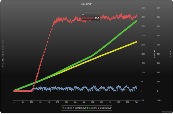
Figure A2. The red and blue lines were the waste generated by members of the brands represented by yellow and green lines, respectively. In this case, the use of a reputation system was clearly correlated to greater fitness loss for polluters (green line) compared to non-polluters (yellow line), especially towards the end of the simulation run. 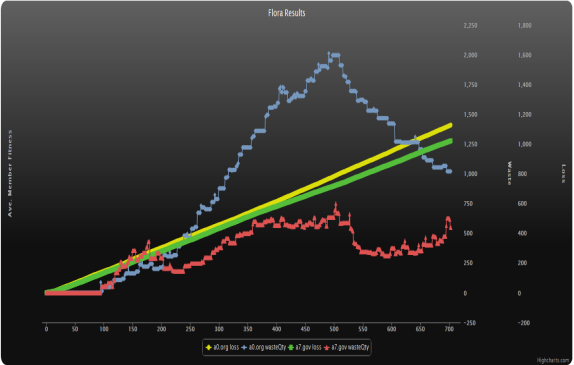
Figure A3. The red and blue lines were the waste generated by members of the brands represented by yellow and green lines, respectively. For this particular run, no reputation system was used and there was not as much difference between the fitness loss of polluters (green) and non-polluters (yellow line). The WASTE_SPREAD_RATE may have been set high enough for pollution to spread rapidly to non-polluter brand locations, leading to nonpolluter locations having more waste than polluter locations, which effectively reversed the relation seen in Figure A2.
Appendix 4: Guidelines for Replicating the Test Scenarios
-
To view examples of configuration settings used for each of the test scenarios, click on the highlighted links given above the run request strings below. Unfortunately, the server load on the linked webhost prevents running the simulations for the specified number of cycles or repeats. It is therefore recommended to use a local machine for attempting replication.
To actually replicate the runs on a local machine:
- If you don't have the Apache web server with mod PHP, download it. For Windows, a quick way to install so is to use http://www.wampserver.com/en. (Note: MySQL is not required in Flora.) For Linux, there is usually a "lamp-server install" command that you could use. Or, use http://www.apachefriends.org/en/xampp.html. If you are adventurous, download Apache and PHP separately, then search for and follow online tutorials.
- Download the Flora source code at https://bitbucket.org/siosonel/flora/downloads. Unzip the files to the document root of your web server. That's it for the install.
- For each of the test scenarios that you to replicate, copy and paste the corresponding run request string from below. Click on the button "Update-String-to-Form" to automatically fill-in the configuration parameters. Click "Validate Request" and then Run when no errors are returned. Running multiple runs for the same test scenario might work by loading http://127.0.0.1/flora/multiRun.php on your browser and appending the run request string to the browser address.
- To process the results, check that there are folders and files created under "(document_root)/flora/results/(run_name)". We converted the JSON output data to CSV format using http://127.0.0.1/flora/analysis/jsonToCsv.php?runName=(run_name_used). Then use a statistical analysis software, such as STATA or R, to efficiently process the data.
Note that the run requests below were created to facilitate replication, but are not guaranteed to automatically lead to exact configurations of the test scenarios in this paper. In particular, each set of results have been saved with the exact version of source code used. Therefore, the working copy must be reverted to an appropriate version for precise replication, which unfortunately would not work with the current user interface which has been developed only in more recent versions. Still, we expect that only minimal work would be necessary to match our method and results using the most current source code version.
I. Test Scenarios with Inventory System Only
A. Effect of Resource Diversity
Number of unique resources: 36
?runName=k12_vary_rID&config=default&repeat=1&popN=48&locN=64&rsrcN=100&maxCycle=30& amp;rId_unique=36&configDiff=&dEngs=k12.k12&infras=Inventory.inven&k12= pq_15,cq_25,wq_100,numP_48,begP_0,numL_64,begL_0,numB_16,prefixB_a,inven_inven&inven=Number of unique resources: 48
?runName=k12_vary_rID&config=default&repeat=1&popN=48&locN=64&rsrcN=100&maxCycle=30& amp;rId_unique=48&configDiff=&dEngs=k12.k12&infras=Inventory.inven&k12= pq_15,cq_25,wq_100,numP_48,begP_0,numL_64,begL_0,numB_16,prefixB_a,inven_inven&inven=Number of unique resources: 64
?runName=k12_vary_rID&config=default&repeat=1&popN=48&locN=64&rsrcN=100&maxCycle=30& amp;rId_unique=64&configDiff=&dEngs=k12.k12&infras=Inventory.inven&k12= pq_15,cq_25,wq_100,numP_48,begP_0,numL_64,begL_0,numB_16,prefixB_a,inven_inven&inven=B. Effect of MIN_0_DIGITS
MIN_0_DIGITS = 1
?runName=k12_vary_MIN_0&config=default&repeat=1&popN=48&locN=64&rsrcN=100&maxCycle=30& amp;rId_unique=64&configDiff=MIN_0_DIGIT~1,&dEngs=k12.k12&infras=Inventory.inven&k12= pq_15,cq_25,wq_100,numP_48,begP_0,numL_64,begL_0,numB_16,prefixB_a,inven_inven&inven=MIN_0_DIGITS = 2
?runName=k12_vary_MIN_0&config=default&repeat=1&popN=48&locN=64&rsrcN=100&maxCycle=30& amp;rId_unique=64&configDiff=MIN_0_DIGIT~2,&dEngs=k12.k12&infras=Inventory.inven&k12= pq_15,cq_25,wq_100,numP_48,begP_0,numL_64,begL_0,numB_16,prefixB_a,inven_inven&inven=MIN_0_DIGITS = 3
?runName=k12_vary_MIN_0&config=default&repeat=1&popN=48&locN=64&rsrcN=100&maxCycle=30& amp;rId_unique=64&configDiff=MIN_0_DIGIT~3,&dEngs=k12.k12&infras=Inventory.inven&k12= pq_15,cq_25,wq_100,numP_48,begP_0,numL_64,begL_0,numB_16,prefixB_a,inven_inven&inven=C. Effect of Hoarders
Hoarder:Nonhoarder = 3:45
?runName=k12u_vary_numP&config=default&repeat=1&popN=48&locN=44&rsrcN=100&maxCycle= 30&rId_unique=64&configDiff=MIN_0_DIGIT~1,&dEngs=k12.k12,k12u.k12u&infras=Inventory.inven&k12= pq_15,cq_25,wq_100,numP_45,begP_0,numL_40,begL_0,numB_1,prefixB_a,inven_inven&k12u= pq_15,cq_25,wq_100,numP_3,begP_45,numL_4,begL_40,numB_1,prefixB_b,inven_inven&inven=Hoarder:Nonhoarder = 6:42
?runName=k12u_vary_numP&config=default&repeat=1&popN=48&locN=44&rsrcN=100&maxCycle= 30&rId_unique=64&configDiff=MIN_0_DIGIT~1,&dEngs=k12.k12,k12u.k12u&infras=Inventory.inven&k12= pq_15,cq_25,wq_100,numP_42,begP_0,numL_36,begL_0,numB_1,prefixB_a,inven_inven&k12u= pq_15,cq_25,wq_100,numP_6,begP_42,numL_8,begL_36,numB_1,prefixB_b,inven_inven&inven=Hoarder:Nonhoarder = 9:39
?runName=k12u_vary_numP&config=default&repeat=1&popN=48&locN=44&rsrcN=100&maxCycle= 30&rId_unique=64&configDiff=MIN_0_DIGIT~1,&dEngs=k12.k12,k12u.k12u&infras=Inventory.inven&k12= pq_15,cq_25,wq_100,numP_39,begP_0,numL_32,begL_0,numB_1,prefixB_a,inven_inven&k12u= pq_15,cq_25,wq_100,numP_9,begP_39,numL_12,begL_32,numB_1,prefixB_b,inven_inven&inven=Hoarder:Nonhoarder = 12:36
?runName=k12u_vary_numP&config=default&repeat=1&popN=48&locN=44&rsrcN=100&maxCycle= 30&rId_unique=64&configDiff=MIN_0_DIGIT~1,&dEngs=k12.k12,k12u.k12u&infras=Inventory.inven&k12= pq_15,cq_25,wq_100,numP_36,begP_0,numL_28,begL_0,numB_1,prefixB_a,inven_inven&k12u= pq_15,cq_25,wq_100,numP_12,begP_36,numL_16,begL_28,numB_1,prefixB_b,inven_inven&inven=II. Test Scenarios with Inventory and Accounting Systems
A. Effect of Number of Brands
LETS Number of Brands = 8
?runName=k13_vary_initBal&config=default&repeat=1&popN=48&locN=64&rsrcN=100&maxCycle=30& amp;rId_unique=64&configDiff=&dEngs=k13.k13&infras=Inventory.inven,Lets.lets&k13= pq_15,cq_25,wq_100,numP_48,begP_0,numL_64,begL_0,numB_8,prefixB_a,inven_inven,acctant_lets&inven=&lets= initBal_500LETS Number of Brands = 24
?runName=k13_vary_initBal&config=default&repeat=1&popN=48&locN=64&rsrcN=100&maxCycle=30& amp;rId_unique=64&configDiff=&dEngs=k13.k13&infras=Inventory.inven,Lets.lets&k13= pq_15,cq_25,wq_100,numP_48,begP_0,numL_64,begL_0,numB_24,prefixB_a,inven_inven,acctant_lets&inven=&lets= initBal_500OCAUP Number of Brands = 8
?runName=k13_vary_initBal&config=default&repeat=1&popN=48&locN=64&rsrcN=100&maxCycle=30& amp;rId_unique=64&configDiff=&dEngs=k13.k13&infras=Inventory.inven,Lets.lets&k13= pq_15,cq_25,wq_100,numP_48,begP_0,numL_64,begL_0,numB_8,prefixB_a,inven_inven,acctant_ocaup&inven=&lets= initBal_500OCAUP Number of Brands = 24
?runName=k13_vary_initBal&config=default&repeat=1&popN=48&locN=64&rsrcN=100&maxCycle=30& amp;rId_unique=64&configDiff=&dEngs=k13.k13&infras=Inventory.inven,Lets.lets&k13= pq_15,cq_25,wq_100,numP_48,begP_0,numL_64,begL_0,numB_24,prefixB_a,inven_inven,acctant_ocaup&inven=&lets= initBal_500B. Effect of Initial Balance
LETS = 500 units
?runName=k13_vary_initBal&config=default&repeat=1&popN=48&locN=64&rsrcN=100&maxCycle=30& amp;rId_unique=64&configDiff=&dEngs=k13.k13&infras=Inventory.inven,Lets.lets&k13= pq_15,cq_25,wq_100,numP_48,begP_0,numL_64,begL_0,numB_16,prefixB_a,inven_inven,acctant_lets&inven=&lets= initBal_500LETS = 1000 units
?runName=k13_vary_initBal&config=default&repeat=1&popN=48&locN=64&rsrcN=100&maxCycle=30& amp;rId_unique=64&configDiff=&dEngs=k13.k13&infras=Inventory.inven,Lets.lets&k13= pq_15,cq_25,wq_100,numP_48,begP_0,numL_64,begL_0,numB_16,prefixB_a,inven_inven,acctant_lets&inven=&lets= initBal_1000Ocaup = 500 units
?runName=k13_vary_initBal&config=default&repeat=1&popN=48&locN=64&rsrcN=100&maxCycle=30& amp;rId_unique=64&configDiff=&dEngs=k13.k13&infras=Inventory.inven,Ocaup.ocaup&k13= pq_15,cq_25,wq_100,numP_48,begP_0,numL_64,begL_0,numB_16,prefixB_a,inven_inven,acctant_ocaup&inven=&lets= initBal_500Ocaup = 1000 units
?runName=k13_vary_initBal&config=default&repeat=1&popN=48&locN=64&rsrcN=100&maxCycle=30& amp;rId_unique=64&configDiff=&dEngs=k13.k13&infras=Inventory.inven,Ocaup.ocaup&k13= pq_15,cq_25,wq_100,numP_48,begP_0,numL_64,begL_0,numB_16,prefixB_a,inven_inven,acctant_ocaup&inven=&lets= initBal_1000III. Test Scenarios with Inventory, Accounting, and Reputation Systems
A. Effect of Type of Screening
No-Screening
?runName=k15_vary_evalDxn&config=default&repeat=10&popN=48&locN=64&rsrcN=100&maxCycle= 30&rId_unique=64&configDiff=WASTE_EFFECT_ON_ADDER~0.002,&dEngs=k15.k15&infras= Inventory.inven,Ocaup.ocaup,BrandIndex.index&k15= pq_15,cq_25,wq_100,numP_48,begP_0,numL_64,begL_0,numB_16,prefixB_a,inven_inven,acctant_ocaup,rater_index,evalDxn_0_0,clean Brand_7,cleanNot_1&inven=&ocaup=initBal_500&index=netBal_-1_1,PNratio_0.5_2.5,revToQty_- 1_1000,px_3,cx_2,wx_3,srcInvens_inven,srcAcctants_ocaup,acctsTTL_1,complaintTTL_50Seller-Screening
?runName=k15_vary_evalDxn&config=default&repeat=10&popN=48&locN=64&rsrcN=100&maxCycle= 30&rId_unique=64&configDiff=WASTE_EFFECT_ON_ADDER~0.002,&dEngs=k15.k15&infras= Inventory.inven,Ocaup.ocaup,BrandIndex.index&k15= pq_15,cq_25,wq_100,numP_48,begP_0,numL_64,begL_0,numB_16,prefixB_a,inven_inven,acctant_ocaup,rater_index,evalDxn_0_1,clean Brand_7,cleanNot_1&inven=&ocaup=initBal_500&index=netBal_-1_1,PNratio_0.5_2.5,revToQty_- 1_1000,px_3,cx_2,wx_3,srcInvens_inven,srcAcctants_ocaup,acctsTTL_1,complaintTTL_50Buyer-Screening
?runName=k15_vary_evalDxn&config=default&repeat=10&popN=48&locN=64&rsrcN=100&maxCycle= 30&rId_unique=64&configDiff=WASTE_EFFECT_ON_ADDER~0.002,&dEngs=k15.k15&infras= Inventory.inven,Ocaup.ocaup,BrandIndex.index&k15= pq_15,cq_25,wq_100,numP_48,begP_0,numL_64,begL_0,numB_16,prefixB_a,inven_inven,acctant_ocaup,rater_index,evalDxn_1_0,clean Brand_7,cleanNot_1&inven=&ocaup=initBal_500&index=netBal_-1_1,PNratio_0.5_2.5,revToQty_- 1_1000,px_3,cx_2,wx_3,srcInvens_inven,srcAcctants_ocaup,acctsTTL_1,complaintTTL_50
Appendix 5: Entity-Relationship Diagram of the TDI Framework
References
-
BERNERS-LEE, T. (2000). Weaving the Web. New York, NY: HarperCollins.
BORNER, K. (2011). Plug-and-Play Macroscopes. Communications of the ACM, 54 (3) pp. 60-69 doi: 10.1145/1897852.1897871. http://cacm.acm.org/magazines/2011/3/105316-plug-and-play-macroscopes/fulltext. [doi:10.1145/1897852.1897871]
DODSON, L., Sterling, R. S., & Bennett, J. K. (2012). Considering failure: eight years of ITID research. Proceedings of the Fifth International Conference on Information and Communication Technologies and Development (ICTD2012), New York, NY:ACM. [doi:10.1145/2160673.2160681]
EPSTEIN, J. M. & Axtell, R. L. (1996). Growing artificial societies: social science from the bottom up. Crawfordsville, Indiana: R.R. Donnelley and Sons Co.
FULLAM, K. K., Klos, T. B. , Muller, G., Sabater, J., Schlosser, A., Topol, Z., Barber, K. S., Rosenschein, J., Vercouter, L., & Voss, M. (2005). A specification of the agent reputation and trust (A R T) testbed: experimentation and competition for trust in agent societies. Autonomous Agents and Multi Agent Systems (AAMAS 05), July, pp. 512-8. [doi:10.1145/1082473.1082551]
GOMEZ, G. M. (2010). What was the deal for the participants of the Argentine local currency systems, the Redes de Trueque? Environment and Planning, Vol. 42 pp. 1669-1685. doi:10.1068/a42309 [doi:10.1068/a42309]
ISHINISHI, M. & Namatame, A. (1999). Testbed for artificial markets. IEEE '99 Conference Proceedings on Systems, Man, and Cybernetics, Vol. 2 pp. 610 -615. [doi:10.1109/icsmc.1999.825330]
LINTON, M., Leach, N., Winkworth, J., Winkworth, M., Soutar, R. & Stewart, N. (1996). Frequently asked questions about LETSystems. http://www.gmlets.u-net.com/faq.html. Archived at http://www.webcitation.org/64tVgkyIZ.
MURRAY, C.J. (1994). Quantifying the burden of disease: the technical basis for disability-adjusted life years. WHO Bulletin OMS, Vol. 1994 72(3) 429-445. http://www.ncbi.nlm.nih.gov/pmc/articles/PMC2486718/pdf/bullwho00414-0105.pdf
NONGAILLARD, A. & Mathieu, P. (2011). Reallocation problems in agent societies: a local mechanism to maximize social welfare. Journal of Artificial Societies and Social Simulation 14 (3) 5. https://www.jasss.org/14/3/5.html
NOWAK, M. A. & Sigmund, K. (1998). Evolution of indirect reciprocity by image scoring. Nature, 393 June 11, 1998, pp 573-577. http://homepage.univie.ac.at/karl.sigmund/Nature98.pdf [doi:10.1038/31225]
SAQALLI, M., Bielders, C. L., Gerard, B. & Defourny, P. (2010). Simulating rural environmentally and socio-economically constrained multi-activity and multi-decision societies in a low-data context: a challenge through empirical agent-based modeling'. Journal of Artificial Societies and Social Simulation 13 (2) 1. https://www.jasss.org/13/2/1.html
SCHLOSSER, A., Voss, M. & Bruckner, L. (2006). On the simulation of global reputation systems. Journal of Artificial Societies and Social Simulation, 9 (1) 4. https://www.jasss.org/9/1/4.html.
SCHROEDER, R., Miyazaki, Y., & Fare, M. (2011). Community currency research: an analysis of the literature. International Journal of Community Currency Research 15 (A) 31-41. http://www.ijccr.net/IJCCR/2011_%2815%29_files/IJCCR%202011%20Schroeder.pdf
SIOSON, E. (2009). OCAUP Accounting Model. http://tyaga.org/docs/ocaup.pdf. Archived at: http://www.webcitation.org/64tUgyhzX.
WHITACRE, J. & Bender, A. (2010). Degeneracy : A design principle for achieving robustness and evolvability. Journal of Theoretical Biology, Volume 263, Issue 1, 7 March 2010, pp. 143-153. http://www.sciencedirect.com/science/article/pii/S0022519309005347#sec1.5 [doi:10.1016/j.jtbi.2009.11.008]
WIERZBICKI, A. & Nielek, R. (2011). Fairness emergence in reputation systems. Journal of Artificial Societies and Social Simulation, 14 (1) 3. https://www.jasss.org/14/1/3.html