
 Abstract
- Human mobility and, in particular, commuting patterns have a fundamental role in understanding socio-economic systems. Analysing and modelling the networks formed by commuters, for example, has become a crucial requirement in studying rural areas dynamics and to help decision-making. This paper presents a simple spatial interaction commuting model with only one parameter. The proposed algorithm considers each individual who wants to commute, starting from their residence to all the possible workplaces. The algorithm decides the location of the workplace following the classical rule inspired from the gravity law consisting of a compromise between the job offers and the distance to the job. The further away the job is, the more important the offer should be to be considered for the decision. Inversely, the quantity of offers is not important for the decision when these offers are close by. The presented model provides a simple, yet powerful approach to simulate realistic distributions of commuters for empirical studies with limited data availability. The paper also presents a comparative analysis of the structure of the commuting networks of the four European regions to which we apply our model. The model is calibrated and validated on these regions. The results from the analysis show that the model is very efficient in reproducing most of the statistical properties of the network given by the data sources.
- Keywords:
- Commuting Patterns, Network Generation Models, Individual Based Models, Stochastic Models
Introduction
- 1.1
- For two decades, not only the number of commuters (i.e. people living in a municipality and working in another) but also, the average distance travelled by workers has increased in most European countries. This makes commuting a fundamental phenomenon in understanding socio-economic macrostructures. The precise description of commuting patterns has a central role in many applied questions: from the studies on traffic and the planning of infrastructures (Ortuzar 2001) to the diffusion of epidemics (Balcan 2009) or large demographic simulations (Huet 2011).
- 1.2
- Despite their importance for describing realistic socio-economic frameworks, datasets describing human commuting patterns are rarely provided by statistical offices. Therefore a large effort has been made to find some algorithmic procedures able to reconstruct commuting flows, starting from the aggregate datasets that are usually available. These are models that simulate the morphogenesis of the network, taking into account the constraints given by the available aggregate data and the geographical properties of the networks. Good reviews of these methods can be found in Ortuzar (2001), in the framework of transport modelling, in Barthélémy (2011), in the framework of spatial networks modelling, and finally in Rouwendal and Nijkamp (2004) concerning micro-economy. On the other hand the field still has many gaps, mostly due to the difficulties met in calibrating the parameters of the proposed models and in finding good descriptions for zones inhabited by small populations. A discussion on the state of the art is provided in section 1.
- 1.3
- Our research takes place in the framework of the European project PRIMA[1]. The microsimulation model developed within the PRIMA project simulates the dynamics of the population living in the European rural (low population density) municipalities. Therefore, one of our main focuses is the commuting structures in the rural areas of our case study regions. These structures had to be analysed and reproduced in the microsimulation model, which aims to help decision-making regarding land-use policies. Thus, we needed a simple commuting network algorithm able to generate the network of the European regions where the detailed commuting data was not available.
- 1.4
- For some of these regions, the only available data at the municipality level consisted of total number of individuals commuting out of the municipality and total number of individuals commuting into the municipality. In these cases, the precise structure of the commuting network was unknown. In other words, the exact flows of individuals going from a municipality where they live to another one where they work was missing. Consequently, these flows had to be recreated on the basis of a set of assumptions. A description of the case studies we analysed is provided in section 2.
- 1.5
- This paper describes the method we used to recreate all the commuting flows. Our method generates a commuting network, using a Monte Carlo simulation approach that can also be applied to low density zones. It is based on the individual choices of the commuters. We propose an extremely simplified framework, inspired by the gravity law, which aims to be general enough to be applicable to areas with diverse geographical features and different commuting structures. Despite its simplicity, the proposed approach is capable of faithfully replicating the structure of observed commuting networks.
- 1.6
- Our algorithm considers each individual who wants to commute, from their living place to all possible workplaces. Individuals decide where they work following a classical rule consisting of a compromise between the job offers and the distances to the jobs. The further away the job is, the more important the offer should be to be considered in the decision. Inversely, the number of offers is less important for decision-making when these offers are in municipalities nearby. We initialize the algorithm with aggregate data on job seekers (i.e., the number of out-commuters) and job offers (i.e., the number of in-commuters) in each municipality. The algorithm memorizes past choices and after a job is associated to a commuter, the local information for the municipalities involved in the choice is updated. The algorithm is repeated until all the jobs are assigned. The details of the model are explained in section 3.1.
- 1.7
- We also provide a method to calibrate the unique parameter of our algorithm, using detailed data from statistical offices. We show that, even if the selected regions are significantly diverse, the parameter does not vary dramatically from one region to another. The calibration method is presented in section 3.2.
- 1.8
- Finally, we provide a quantitative framework to compare the network observed by statistical offices with the generated structures of our algorithm (Section 4). In particular, we articulate the validation systems at two levels. In section 4.2 we focus on the global topological properties of the network, such as the probability distributions of important network indicators (e.g., degrees and weights). In section 4.3, we introduce a statistical framework that allows a comparison, at the local level, of the similarity between the flows observed in the real case against those present in the generated network.
- 1.9
- An implementation of the algorithm in NetLogo, provided as additional material and detailed in the appendix, allows a graphical representation of the generation model.
Background
- 2.1
- The literature on the construction and use of commuting networks is abundant; both from the point of view of the analysis of the structures, and from the point of view of the models (see the reviews of Ortuzar 2001; Barthélémy 2011; Rouwendal and Nijkamp 2004 in various research domains).
- 2.2
- Many recent papers adopted an approach based on network theory. An interesting and complete analysis of the commuting structures from this point of view was introduced in De Montis et al. (2007; 2010). In this framework, most importantly concerning the modelling issues, the question about the commuting networks is set in the larger conceptual category of spatially constrained network structures. This kind of analysis concerns not only commuting, but all the situations where the geography has a significant role: from the reconstruction of migrant patterns (Lemercier and Rosental 2008) to the analysis of the internet at autonomous system level (Pastor-Satorras and Vespignani 2004), to airline network structure (Barrat et al. 2004). A particularly important study in this context is Barrat et al. (2005) where the concept of "preferential attachment" (Barabasi and Albert 1999) is adapted in order to consider not only the strength of a node given by its current in-degree, but also the spatial constraint included in the journey-to-work network.
- 2.3
- A more classical approach comes from the micro-economists (Rouwendal and Nijkamp 2004). Starting from the monocentric model of residential location proposed by Alonson (1964), economists and geographers in urban modelling initially did not consider the space as determinant in residence location of the individual, assuming that places of work are all located in the centre of a unique city. In the same way, looking at the decision regarding the job, job search theory does not take especially into account the distance of commuting in its first formalization. It assumes a worker's optimal strategy is simply to reject any wage offer lower than a reservation wage, and accept any wage offer higher than this reservation wage. However, commuting time was soon included in new job-search models as in (Van Den Berg and Gorter 1997). In this model, a job offer consists of a wage and a commuting time pair. To be applied, this approach requires data on wage offers and their locations. When working with models at very local level (e.g., municipalities or villages), wage data is often difficult to obtain.
- 2.4
- However, the most used approach to the modelling of commuting or migration structures is the one based on the so-called gravity law models (Haynes 1988). The term gravity law is a metaphor from classical physics. We can imagine that as it happens in gravitation, the interaction between two municipalities depends proportionally on a parameter: for example, the size of the municipality (equivalent to mass in the gravitational law), and in inverse proportion with some power law of the distance. It is recognized that the concept of "distance" can be formulated as something other than a real geographical or spatial category: it can be a travelling time, a topological distance on a network, but also a "social" distance (e.g. the cases of border cities where different languages are spoken). The classical formalization of probability pij of a commuter to live in the municipality i and to work in the municipality j is the following:
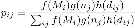
(1) where we consider different proportionality parameters Mi, Nj, respectively for the origin and destination municipalities (this size could refer to the area of the municipalities, its population or the number of working people) and the distance between each pair of municipalities dij.
- 2.5
- Using this probability model, it is possible to determine the traffic between each pair of municipalities with different methods (e.g. IPF, multinomial models, etc.). We notice that the functions f(Mi), g(Ni) and h(dij) may assume any possible shape. For h(dij), the literature generally agrees that an exponential specification appears to fit better with reality. However, in some applications, a power law decay often seems to be a better fit (De Montis 2007, 2010; Reggiani and Vinciguerra 2007). Some studies propose a combined form of the two (Ortuzar and Willusem 2001), or a different form (de Vries et al. 2009), in order to better fit the empirical data.
- 2.6
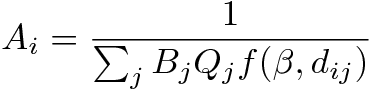
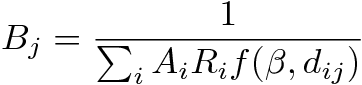
- The most common applied model of spatial interaction to generate commuting networks is the so called "doubly-constrained" model (Wilson 1998; Choukroun 1975). Based on the gravity law, it predicts the number Tij of journeys-to-work between any pair of origin (i) - destination (j) zones considering the number of out-commuters of i and the number of in-commuters of j:
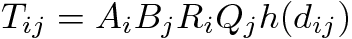
(2) where:
- 2.7
- The factors Ai and Bj ensure that the Tij table is consistent with the exogenous rows and columns totals. These balancing factors, plus a distance parameter β, implicit in the function h(dij),have to be calibrated. An entropy maximization approach allows calibrating such model considering only one parameter to find (β) since Ai and Bj are automatically solved by this method. This optimization approach consists in associating any particular microstate with a macrostate, which is simply the number of trips from an origin to a destination. A macrostate is feasible if it reproduces known properties referred to as system states (for example, the total number of travelers). Estimating the solution of the model consists in finding the macrostates, maximizing a chosen distance function of the considered macrostate to the observed data among the feasible macrostates (Bernstein 2003).
- 2.8
- Several improvements were proposed based on this doubly-constrained model. In Fotheringham (1981), a competing destination model is introduced to improve the spatial structure of the generated network. Fik and Mulligan (1990) extend this competing model to measure the accessibility of a destination related to destinations of the same hierarchical order in the system of central places (founded on the Central Place Theory). They also incorporate a measure that relates to the number of intervening opportunities from the living place i to the attractive force j. These intervening opportunities are the potential destinations within a distance smaller than dij. To go beyond the gravity law models' weaknesses, some authors developed an approach founded on the network paradigm (Thorsen et al. 1999; Gitlesen 2010). This kind of procedure has the disadvantage of increasing the number of parameters, which is what we wanted to avoid.
- 2.9
- Very recently, Simini et al. (2011) proposed an algorithm free of parameters to generate many different spatial networks. They consider the job demand and the job offer as a part of the population of the origin-destination zones, and compute the probability of a flow between the origin i and the destination j, considering these parts and the density of people living between i and j. They apply this principle for the generation of the commuting network of USA at the county level. This model is very interesting, nonetheless we doubt its suitability to reproduce a commuting network at such a low level as the municipalities in our study regions (such as France, where the average size of an Auvergne municipality is 1024 inhabitants). Though this model addresses similar issues, the authors conclude the lack of an effective distance weakens their model fitness.
- 2.10
- Our study analyses different regions from various countries. Regions are defined as sets of NUTS3[2] areas for each country; these regions vary in size, population, and other economic and social properties. We are interested in the inter-municipality commuting network. Very few papers deal with this topic on a small scale. Some studies analyse the inter-municipality commuting network (De Montis 2007, 2010), showing that the Sardinian and the Sicilian inter-municipal commuting networks exhibit a traffic property based on a power law with exponent 2. Others, such as Thorsen and Gitlesen (1998), compare different spatial interaction models by an empirical evaluation of the municipalities of a Norwegian region. One study analyses at the district level (which is higher than the municipality level) the German commuting network (Patuelli et al. 2007), using a comparison of two spatial interaction models. The set of publications shows the interest in such an approach to study the evolution of these types of networks over time.
- 2.11
- For the presented model, the individual choice for a job location is probabilistic. Decisions are mainly stochastic, and so is the model. Each time the model is run, we obtain a different network based on the statistical properties used as input. This should be contrasted with the generation of an optimized network making deterministic the flow between the related municipalities. Especially for the latter, a deterministic approach does not appear relevant, since the local commuting choice is influenced by many local decisions which can be seen as random variations. The validation of the model shows that we obtained a good fit of the network given by the observed data. These results are very stable; the stochasticity of the model thus reflects local diversity without perturbing the statistical properties of the network. For the deterrence function, we decided to use a power law; nevertheless, another function could be tested.
Regional commuting network structures - Specific differences and global properties.
- 3.1
- The first part of our study concerns the analysis of our study regions. The local statistical offices[3] provide all the information necessary to characterize the structure of the commuting network. We consider: two separated NUTS2 regions in France (Auvergne and Bretagne), each composed of four NUTS3 regions; a group of two NUTS3 regions in the UK (Nottinghamshire and Derbyshire); and a group of two NUTS3 regions in Germany (the Altmark region is composed by the districts of Stendal and Salzwedel). Differences between the data availability within regions must be noted, as the data for Auvergne and Bretagne is much more comprehensive, in comparison to the other two case study regions. Indeed, data describing the commuting flows between each pair of municipalities with less than 10 commuters is not available in the German data (Altmark) and the simlar flows smaller than 3 are not available in the English data (Nottinghamshire and Derbyshire).
- 3.2
- The selected regions differ on many aspects: the number of municipalities, geographical structure, and socio-economic characteristics. They were chosen by the European project because they are all rural regions with diverse socio-economic characteristics. Table 1 presents some basic characteristics of each case study.
Table 1: Characteristics of selected study regions Region Number of municipalities Average size of a municipality (by number of inhabitants) Average inter-municipality distance (in km) Number of commuters living and working in the region Part of commuters living in and working outside the region Total area surface (in km2) Auvergne (France) 1310 1024 88 261822 7.73% 26,013 Bretagne (France) 1269 2447 99 608587 7.32% 27,208 Altmark (Germany) - subregions 91 2527 50 16770 66.82% 4,715 Nottinghamshire /Derbyshire (UK) 372 5300 44 573022 12.4% 4,839 - 3.3
- The objective of this first analysis is to determine the characteristics of the commuting networks composed by the regional commuting flows that are present in each region. For this analysis, we create a commuting matrix from a dataset containing the number of individuals that commute (i.e. reside in one settlement and work in another) within each of the selected regions. A representative section of the matrix used is shown in Table 2. Each row represents the place of residence and each column represents the working place; the cell at the intersection of each row and column contains the number of persons living and working in the corresponding row and column. For our analysis we ignore the cells in the diagonal of the table, as they represent non-commuting individuals (i.e., persons living and working in the same place).
Table 2: Example of commuting data from the Altmark Region Municipality of employment Municipality of residence 81026 81030 81035 81045 81080 81095 ... 81026 0 0 0 0 0 0 ... 81030 0 0 0 3 0 0 ... 81035 0 0 0 2 0 0 ... 81045 0 2 2 0 2 2 ... 81080 0 0 0 0 0 0 ... 81095 0 2 0 8 0 0 ... ... ... ... ... ... ... ... 0 - 3.4
- After analyzing some global properties of the network structure we observe that the presented regions have quite dissimilar structures. The first analyzed property of the networks concerns the distributions of the degrees. The degree is a property of the associated un-weighted network. For the construction of the un-weighted network we consider all the municipalities and add a directed link between the municipality i and the municipality j if at least one individual commutes from i to j. The in-degree of a municipality i (kin(i)) is the number of links entering in i, while the out-degree (kout(i)) is the number of links starting from i.
- 3.5
- The probability distributions of the "in and out" degrees are represented in figures 1. As we can observe on these figures, the different case studies are characterized by very different behaviours according to the degree distribution.
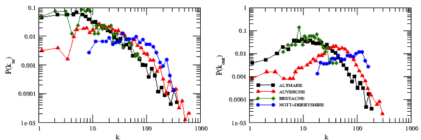
Figure 1. In and Out degree distributions of each case study region - 3.6
- The out-degree distribution shows that the municipalities in the UK region always have a large and uniform degree distribution. This can be explained by the fact that for the UK, the number of commuters is extremely large, and the network is very dense in terms of links. This kind of uniform structure can be connected to the lack of "working hubs" able to attract workers more strongly than the other municipalities. This corresponds with what we observe in the in-degree distribution where we see that few municipalities have a small in-degree while a considerable part has a high in-degree.
- 3.7
- The situation in Auvergne and Bretagne, where the in-degree distributions suggest the presence of real "working hubs" in the commuting network (a small but not unimportant part of municipalities reached much more than the others) is totally different.
- 3.8
- For the Altmark region, the total number of connections is generally lower, suggesting that this region represents only a part of a larger commuting network. This can be explained considering that the majority of commuters in the studied region work outside this region (66.82% as shown in Table 1).
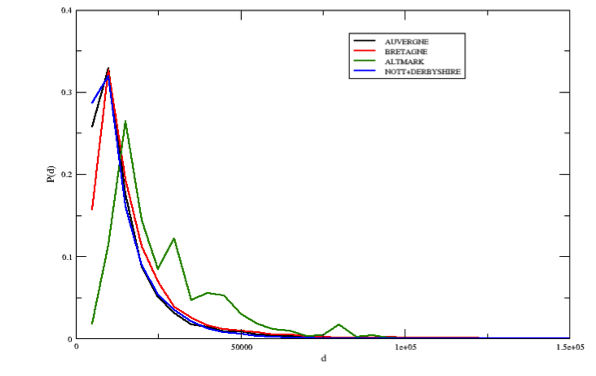
Figure 2. Distribution of the commuting distances (in meters) for the selected case studies - 3.9
- Another important consideration concerns the distribution of distances covered by the commuters. This measure is presented in Figure 2.
- 3.10
- The distribution of the distances shows that in the UK regions, smaller distances are favoured. This confirms our intuition that job offers are homogeneously distributed among all the municipalities in the region (thus, there are no working hubs). For this reason people do not need to travel long distances to find a job. The opposite situation is observed in the Altmark case, where a significant share of the commuters can travel up to 80 km.
- 3.11
- In this section we provided a brief description of the selected case studies. We showed the structural differences and global properties of the studied commuting networks. In the following section we present a method to construct a synthetic network, based on the decision of the individual workers. This method is then used to generate commuting networks for regions where the detailed commuting data is not available.
A Monte-Carlo simulation approach to generate realistic commuting networks
- 4.1
- The usual methods for reconstructing the structure of commuting networks are based on the gravity law. The main hindrance of this approach is that it is not easy to calibrate the gravity law model (Williams 1976). Moreover, it is a deterministic method which appears inappropriate when flows for small municipalities must be predicted, as it is the case for our study regions. We propose a simple network generation model that presents a higher level of universality and which can be applied with a good degree of confidence to all the case study regions.
The individual-level generation model
- 4.2
- The model is based on the individual choices of the commuters, namely people in the active class that do not work in the municipality where they reside.
- 4.3
- When looking for an occupation outside of the living place, two factors can influence the choice of the destination: the distance of the potential workplace and its "attractiveness" (defined by the number of jobs it offers). The further away the possible destination is, the more its attractiveness will matter in the decision. If the possible destination is near, the settlement attractiveness becomes less significant for the individual's decision for a workplace.
- 4.4
- We start from a typology of data that is usually available, for each municipality, in each case study:
- the total number of out-commuters (Ri), also called the job demand of the municipality i,
- the total number of in-commuters (Qi), also called the job offer (or attractiveness) of the municipality j,
- the distances among each couple of municipalities (dij)
- 4.5
- In the presented study we use the Euclidean distances in km to describe the distances. Similar results can be obtained using, for example, the road distance or travelled time measures. Some performed test on the results showed that the algorithm is robust to the choice of other distance definitions.
- 4.6
- To each commuter residing in each municipality i, the algorithm associates a working destination j according to the job offers of all the municipalities different from i in the region and the distance between the municipality i and all the possible destinations. The algorithm for the generation of the network evolves according to the following steps:
For each remaining commuter who has not already found a place to work, we:
- Select a residence municipality i at random among the municipalities where there is at least one out-commuter (Ri>0)
- Select the working destination j randomly following the probability distribution given by:
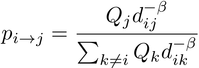
(3) - Update the number of out-commuters of i and the number of in-commuters of j: Ri=Ri-1, Qj=Qj-1
- Recalculate thePi→j distribution
- 4.7
- Different values of the parameter β produce different distance and degree distributions for the generated networks. We calibrate the parameter for the case studies where the complete information in the network is known, in order to have the same distance distribution as the one observed for the real network.
- 4.8
- Analysing the calibration on the regions where the data is available, we observe that with an appropriate choice of the parameter β we are able to generate a commuting network with statistical properties which are very similar to the real network. The calibration procedure and the analysis of the accuracy of the generation algorithm are presented in the following sections.
Model calibration
- 4.9
- The proposed model depends on the spatial parameter β which represents the relative importance of the distance to the destination when choosing a working place. A typical property that distinguishes commuting networks is the distribution of the travelled distance for each worker. We employ this information to calibrate the parameter β. In fact, each value of β produces a network with a typical distance distribution, as it is displayed in Figure 3 for the Auvergne case study.
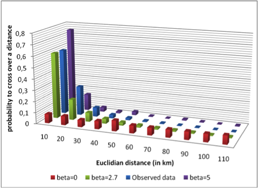
Figure 3. Distance (d in KM) distribution for the real network and three different β values for the Auvergne case study - 4.10
- We observe that, for excessively low values of β the preference toward distant working places is overestimated, while for excessively high values, the choice of close places is overestimated. We calibrate β in order to minimize the distance between the generated travelled distance distribution and the one obtained from the observed data. The minimized distance is the Kolmogorov-Smirnov distance:

(4) where Pco|g(d) are the cumulative distance distributions for the observed (o) and generated (g) networks.
- 4.11
- For each case study we calculated this distance for different values of β and chose the minimum of the function ⟨DKS⟩(β) as the calibrated parameter value. Indeed, to choose the parameter value, we considered ⟨DKS⟩ since the model is stochastic. The value of ⟨DKS⟩ is obtained by calculating the average of the DKS, measured on 100 replications of the generated network for each β value. Within these replications, the variation of the measured DKS is very low, at most 1.13% of ⟨DKS⟩. The calibration process is described in Figure 4. Each dot corresponds to a tested value of β (with a step of 0.5 from 0 to 7 for β, and with a step of 0.1 from 2 to 3 for the ⟨DKS⟩ values required to identify the minimum). Figure 4 shows that for the analyzed regions, the value of β lies in the range [2, 3].
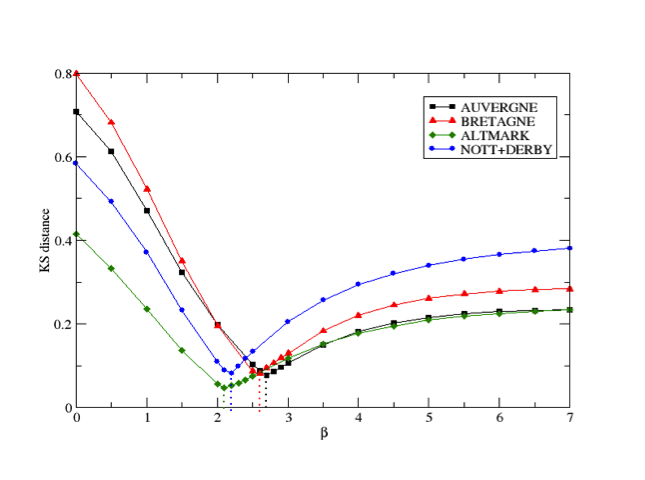
Figure 4. Calibration process results for the four case study regions based on the minimization of the average Kolmogorov-Smirnov distance over 100 replications (each dots represents the result for a tested β value.) - 4.12
- Table 3 lists the optimal values for all the studied regions, where the ⟨DKS⟩ distance is minimized.
In the analyzed regions, notwithstanding the relevant geographic and demographic differences, the coefficient varies slightly in the interval β ∈ [2,3].Table 3: Optimal values of β for the studied regions Region β Auvergne 2.71 Bretagne 2.59 Altmark 2.1 Nottinghamshire and Derbyshire 2.2 - 4.13
- Moreover, we can observe that for all the regions in the whole considered interval, the average KS distance ⟨DKS⟩ between the observed distribution and generated ones is always small. This suggests a strategy for applying this algorithm to the cases where the calibration datasets are not available. A stochastic procedure where at each replication the β value is randomly extracted in the interval β ∈ [2,3] can reproduce, with a good approximation, the commuting patterns of the region. This last assumption is valid only if the considered region is sufficiently isolated; that is, if the total number of commuters, in and out from a municipality, commute to other municipalities within the same region.
Validation
- 5.1
- To assess the quality of the generated network, we compare its properties to the properties of the observed network (i.e., data obtained from the regions' corresponding National Statistical Office).
- 5.2
- Two different kinds of properties are investigated: a first group is measured on the municipality network where we consider that two municipalities are linked when at least one worker commutes between them, whatever the origin-destination is (i.e., considering an unweighted network); a second one is measured on the weighted network which has direct links weighted by the number of individuals commuting from a given municipality to another one.
- 5.3
- For the unweighted network, two different indicators are considered:
- The ability of the generated data to fit the observed in and out degree distributions of the "municipality" network;
- The traffic density distribution describing the density of each weight that can be associated to an undirected link. For an arc between two municipalities, this weight is the sum of the individuals going from one municipality to the other in both directions through the arc.
- 5.4
- For the weighted network, we compare the number of commuters of both the generated and the observed network.
- 5.5
- All these statistics were not used to generate simulated networks. Moreover, we must remember that the number of people looking for a job in a municipality i (Ri) and the job offers in a municipality j (Qj), are reproduced precisely in all municipalities by the generation algorithm.
The properties of the municipality network (i.e. the unweighted network)
- 5.6
- We consider three variables to describe the topological properties of the network and the characteristic of the commuting flows: the in and out degree distribution (p(kin) and p(kout)) and the traffic distribution (p(T)). These indicators are influenced by the choice of the parameter β. As we can observe in Figure 5 for the Auvergne case study, for β = 0 (i.e., when the geography is not important), higher network degrees and lower traffics are observed. As the geography becomes more important (i.e., as β is increased) the maximum network degree decreases and the maximum amount of traffic increases. When distance is not important, people choose their working destination in a wider range of available municipalities. On the contrary, a strong distance constraint forces to choose only between the nearby municipalities. As a consequence of this, traffic on this smaller number of connections will also be globally higher.
- 5.7
- For the Auvergne case study, Figure 5 shows the comparison of the generated and the observed data. It can be seen that, the distributions at the calibration point (β = 2.7) fit the distributions of the observation network perfectly. This fitness should be observed, considering that none of the three measurements (in-commuting degree, out-commuting degree and distribution of traffic), are used by the model; thus, the fitness of the generated network to the observed one is a positive assessment of the effectiveness of the model.
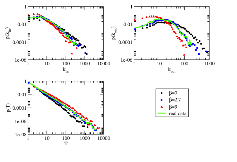
Figure 5. In (kin) and out (kout) degree distributions and traffic (T) distribution for some generated networks with various values of β and for the observed network for the Auvergne case study. The results for the generated networks are averaged on 100 replications of the generation algorithm - 5.8
- Figure 6 shows the comparison between these measures for the observed network and the generated ones for the other case studies. As we can notice in these figures, the traffic (T) distribution is well reproduced in all the case studies. It is not the case for the degree distributions in the UK case study where the generation process completely fails in the estimation. We attribute this discrepancy to the quality of the Census data. Indeed, in UK, a small-cell adjustment method (Stillwell and Duke-Williams 2007) is applied to prevent disclosure of personally identifying data. In particular, this method suppresses some commuting data by replacing values of 1 and 2 with 0 or 3. This adjustment makes the definition of a link between two municipalities different in the model beyond the data and in the generated network through our algorithm. According to the census data, two municipalities are linked only if at least three individuals commute among them. In our generated network, they are linked if at least one individual commute among them. A large number of municipality pairs are, in reality, linked by only one or two individuals. Such pairs are underestimated in the real UK data. We believe this is the reason why the model seems to overestimate the connectivity between municipalities.
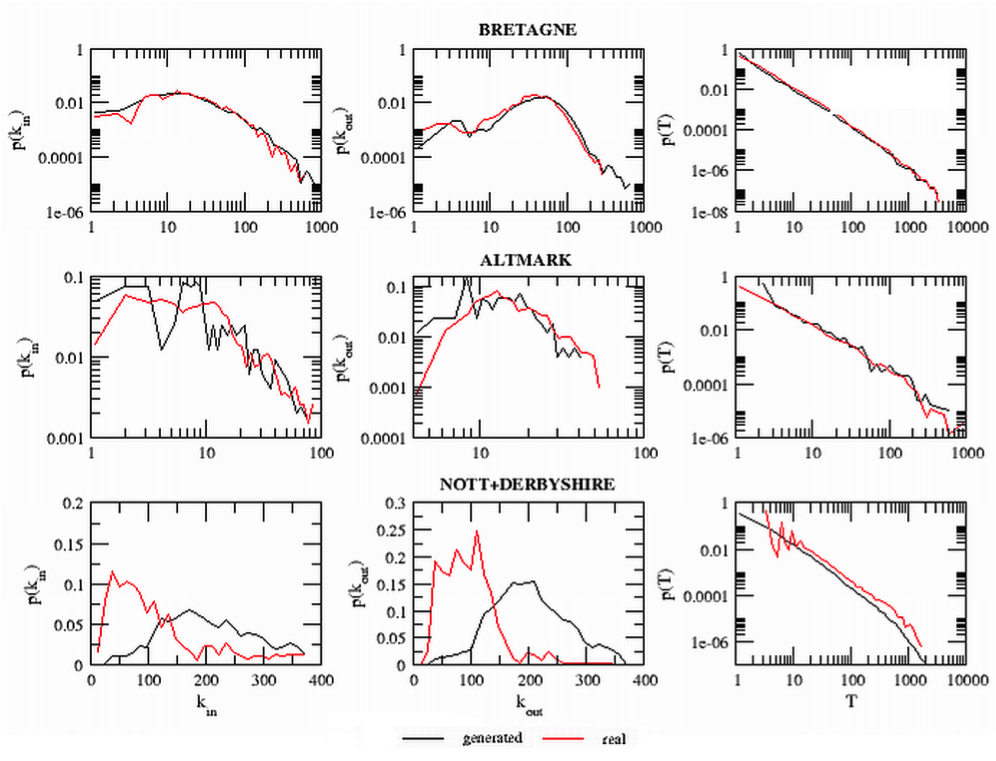
Figure 6. In (kin) and out (kout) degree distributions and traffic (T) distribution for the generated networks at the calibration point and for the real network for the Bretagne, Altmark and UK case studies. The results for the generated networks are averaged on 100 replications of the model The common part of commuters of the weighted network
- 5.9
- We now define an indicator to compare the generated commuting network and the observed commuting network. The statistical offices of France, Germany and United Kingdom provided the observed commuting networks. Assuming that Mn(N) is the set of all possible networks for a set of municipalities. Let O ∈ Mn(N) be one commuting network when Oij is the number of commuters from municipality i to municipality j. Let G ∈ Mn(N) be another commuting network between the same set of municipalities where Gij is the number of commuters from municipality i to municipality j.
- 5.10
- To assess the similarity of flows between the generated and the observed networks, we can compute the common part of commuters (CPC) (Eq. 7) from the number of common commuters (NCC) between O and G (Eq. 5) and the number of commuters (NC) in O (Eq. 6). The CPC appears to be a good indicator of the prediction quality. This indicator may be seen as a simplified variant of the Sørensen index, with the two compared matrices having the same size. The CPC was chosen for its intuitive explanatory power: it is a similarity coefficient which gives the likeness degree between two networks. Its value ranges from 0, when there are no commuters flows in common in the two networks, to a value of 1, when all commuters flows are exactly identical in the two networks.
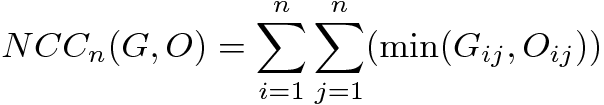
(5) 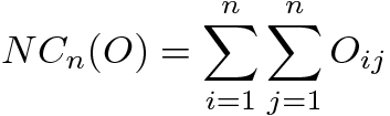
(6) 
(7) - 5.11
- This gives us an indicator to directly compare one replication of the generated network with the observed one. We do the same with all the 100 replications for a given β value and compute the average of the obtained 100 CPC to evaluate the quality of the model. Within the 100 replications, the CPC varies at most, by 1.76% of the average; this means that the stochastic model is very stable (i.e., the stochasticity does not have a significant effect on the properties of the network).
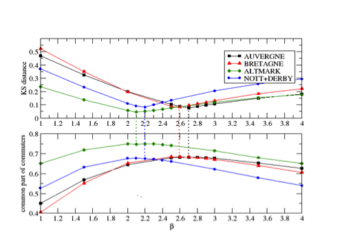
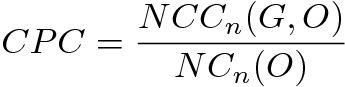
Figure 7. Common part of commuters (at the bottom) for different β values for each case study region (compared to the calibration graph of the Figure 4, presented above) - 5.12
- Figure 7 presents the average CPC for each region and for different βvalues. It is noticeable that the best value of the average CPC function is very close to the one given by the calibration value of β for all the studied regions. This point is stressed in Figure 7 by the dotted line showing the match between the average CPC value and the minimum of the DKS. The proximity, in terms of β of the minimum of the DKS function with the maximum of the CPC function, is surprising and reinforces the idea the CPC is a good quality indicator. We also notice that the best values for both, the DKS and the common part of commuters, varies when defining the model parameter between β= 2 and β = 3. Also, the results from the CPC indicator reinforce the suggested method for the generation of a network in the case where the data is not directly available. In fact, for any point in the interval β ∈ [2,3], and for all the considered regions, the CPC value never goes below CPC=0.6, showing that the generation process yields networks that match the observed network with good accuracy.
- 5.13
- Table 4 shows the average CPC for each case study region and the optimal β value. Results are encouraging: average CPC values fall between 0.67 and 0.76. On average we obtained about 70% of commuters in common. It means that 70% of the observed network is returned by the model. One may also notice that the optimal β value seems to vary in the same way as the average inter-municipality distances of the region (see table 1), for which the Germany and the UK regions both have a small value, whereas the Auvergne and the Bretagne regions, both show a large value.
Table 4: Average Common Part of Commuters for the four case study regions Region β Average Common Part
of CommutersAuvergne 2.71 0.683 Bretagne 2.59 0.684 Altmark 2.1 0.751 Nottinghamshire and Derbyshire 2.2 0.676
Discussion and conclusions
- 6.1
- We propose a very simple stochastic individual-based model able to generate a commuting network with good accuracy. This model is based on the doubly-constrained model proposed by Wilson (1998) and has its roots on the so-called gravitational laws (i.e., consider that individuals tend to "gravitate" towards more attractive areas). It is built on the same principles: an individual tends to choose a job location depending on the job offers and the distance to the offer. The effect of the distance decreases as the distance increases, following a function that we have chosen as a power law. Our model has only one parameter which can be easily calibrated. It ensures that the number of out-commuters and in-commuters for each municipality is respected without needing to solve an optimization problem. However, it must be stressed that our proposed model does not try to reconstruct the exact structure of a commuting network. Achieving this would require considering additional local properties, which are very specific for each region. Instead, we aimed to create a model that can generate realistic synthetic networks from a limited set of data (number of in-commuters and out-commuters on each municipality), which can be used in cases where the detailed commuting data is unavailable. Moreover, reproducing exactly a network at a very low level, especially for very small municipalities (e.g., around 1000 inhabitants on average in some French regions or less than 200 for the studied German region) makes no sense since very small commuting links between small municipalities can result from stochastic factors that cannot be captured with a real deterministic law. As our algorithm is stochastic, it obtains many possible combinations of generated networks respecting the total local commuting flows. This approach seems more relevant than a deterministic approach for modelling a commuting network at the municipality level.
- 6.2
- Our algorithm is validated on four case-study regions situated in France, Germany and the United-Kingdom. We compare the properties of the observed network given by the complete origin-destination table to those of the generated networks. We conclude that the in and out degree distributions of the municipality network, the traffic distribution of the same network are well fitted by the generated networks' distributions. Moreover, the common part of commuters of a generated network with the observed network (i.e., the complete origin-destination table) appears high for all the case study regions. Incidentally, we have noticed that the optimal parameter value of our algorithm is very close to the parameter value that yields a higher value of common commuters.
- 6.3
- The proposed model appears quite relevant for our main problem. Nevertheless, we must remember that aggregated statistics available at the municipality level correspond to all the in-commuters and all the out-commuters of each municipality. This includes commuters that live or work outside the region (i.e., in other municipalities not included in the network). To be sure that our model produces a representative network, it has to be applied on a region where these commuters linked to the outside represent an insignificant part of the total number of commuters. In other words, the region should be what Paelinck and Nijkamp (1975) called a "polarized region": "a connex area in which the internal economic relationships are more intensive than the relationships with respect to regions outside the area" (Cörvers et al. 2009; Konjar et al. 2010) .
- 6.4
- In spite of this limitation, it is apparent from the results of the analysis of the Altmark network (a region where 66.82% of the workers commute outside the region) that the similarity of the generated and real network is good (as shown in the analysis of Figure 7). However, we have to keep in mind that the data regarding the commuting flows smaller than 10 are not available for the Altmark region, and currently we do not know how this limitation impacts on the results. Two issues have affect on the proposed method when the used data includes individuals residing or working outside the region. On the one hand, the model will tend to overestimate the traffic within municipalities, as residents who ought to work outside are distributed within network municipalities. On the other hand, the number of connections may be underestimated as residents occupy jobs which should be taken by individuals living outside the region (thus, leaving municipality with low attractivity without in-commuters).
- 6.5
- Such limitations may be addressed with the use of additional data detailing the number of individuals commuting from or to places outside the region. Alternatively, it is possible to conclude through aggregated data at the regional level or expertise, whether a region is sufficiently independent from another regarding the labour market.
- 6.6
- The second issue concerns the model calibration. Most of the known power-law networks have an exponent value situated between 2 and 3. Our first case studies seem to show that the exponent of our power-law deterrence function varies in the same range. We notice that the error remains quite low between these two boundaries for β.
- 6.7
- A further possible analysis involves testing the quality of an algorithm free of parameters proposed by Simini (2011), even if it does not take directly into account the number of commuters. Such algorithm should be tested on sparsely populated regions such as the ones we worked on (i.e., at the municipality level). They apply this principle for the generation of the commuting network of USA at the county level. This model is very interesting; albeit we question its quality to reproduce a commuting network for very local regions the ones we studied.
- 6.8
- Finally, the model could be improved by the use of other types of distances (such as the commuting time between municipalities). Although our results show that even using a measure such as the Euclidean physical distance (in the case of French regions, or a driving distance (in the case of the Germany region), the model generates networks with similar properties of those observed by the real data. Such refinement is usually limited by the lack of distance data (in this case, commuting time) for the regions. Furthermore, it may be possible to select a better value of β if additional case study regions with geographical and socio-economic differences are analysed.
Appendix: Implementation of the model in the NetLogo framework
- A.1
- An example implementation of the model is included to illustrate how the model works. The implementation was performed in NetLogo 5.0RC4[4] and may run in previous versions (it was successfully tested in version 4). The implementation provides a way to visualize the generation of a network from two input files containing the in-commuting and out-commuting information for each municipality in a region and the distances between each pair of municipalities.
- A.2
- As mentioned, the model requires two input files to run:
- The commuters file named commuters.csv: Which should contain a list of municipalities (one for each line in the file) and the number of individual who commute-out and commute-in (in that order) for each municipality. Each column must be separated by one blank space.
- The distances file named distances.csv: Which should contain the distance between each pair of municipalities as a three column row containing the origin municipality, the destination municipality, and the distance between the pair (in that order). Each column should also be separated by a blank space.
- A.3
- The interface of the implementation is shown in Figure 8. Prior to starting a simulation the beta parameter must be set in order to define the weight of the distance in the commuting decision. For illustrative purposes the proportional-sizes control is provided to present each municipality (depicted as a house in the interface) with a size relative to the initial number of in-commuters (job availability).
Figure 8. Interface of sample model implementation in NetLogo - A.4
- The buttons go and go-forever are used to run the simulation for one step or for a continuous loop (until the total number of commuters has been processed). The update-layout button runs a network layout procedure until pressed again; this may be used to improve the visual position of the network (it does not have any effect on the simulation results).
- A.5
- Results are reported in the three provided charts, which show the distribution of in-commuters, out-commuters, and traffic (number of links with a number of commuters are present). The number of processed commuters and the total number of commuters read from the input files is also shown.
Acknowledgements
- The work of F. Gargiulo is funded by the French ANR project SIMPA. The research leading to these results has also received funding from the European Commission's 7th Framework Programme FP7/2007-2013 under grant agreement n 212345.
Notes
-
1PRototypical policy Impacts on Multifunctional Activities in rural municipalities - EU 7th Framework Research Programme; 2008-2011; https://prima.cemagref.fr/the-project
2The Nomenclature of Territorial Units for Statistics. NUTS 2 corresponds to European basic regions for the application of regional policies and NUTS 3 to small regions for specific diagnoses. For more details, see http://epp.eurostat.ec.europa.eu/portal/page/portal/nuts_nomenclature/introduction
3In France: thanks to the Maurice Halbwach Center, which made available the complete French origin-destination tables for commuters in 1999. In Germany: Commuting data was purchased from the German Federal Employment Agency (Bundesagentur für Arbeit) for the year 2000. In the United Kingdom: Origin-destination data was obtained via the Office for National Statistics NOMIS online database (https://www.nomisweb.co.uk/) for the year 2001.
4 http://ccl.northwestern.edu/netlogo/
References
-
ALONSON, W. (1964), Location and Land Use: Toward a General Theory of Land Rent. Cambridge: Harvard University, 204 pages. [doi:10.4159/harvard.9780674730854]
BALCAN, D., et al. (2009), 'Multiscale mobility networks and the large scale spreading of infectious diseases', Proc. Natl. Acad. Sci, 106 (51), 21485-89. [doi:10.1073/pnas.0906910106]
BARABASI, A.L. and Albert, R. (1999), 'Emergence of Scaling in Random Networks', Science, 286 (5439), 509-12 [doi:10.1126/science.286.5439.509]
BARRAT, A., Barthélemy, M., and Vespignani, A. (2005), 'The effects of spatial constraints on the evolution of weighted complex network', Journal of Statistical Mechanics: Theory and Experiment, P05003, 11. [doi:10.1088/1742-5468/2005/05/p05003]
BARRAT, A., et al. (2004), 'The architecture of complex weighted networks', Proc. Natl. Acad. Sci. , 101, 37-47. [doi:10.1073/pnas.0400087101]
BARTHÉLÉMY, M. (2011), 'Spatial Networks'. Physics Reports 499:1-101, arXiv 1010.0302v2.
BERNSTEIN, D. (2003), 'Transportation Planning', in W.F. Chen and R. J.Y. Liew (eds.), The Civil Engineering Handbook (Boca Raton, London, New York, Washington D.C.: CRC Press LLC).
CHOUKROUN, J.M. (1975), 'A General Framework for the Development of Gravity-type Trip Distribution Models', Regional Science and Urban Economics, 5, 177-202. [doi:10.1016/0166-0462(75)90003-4]
CÖRVERS, F., Hensen, M., and Bongaerts, D. (2009), 'Delimitation and coherence of functional and administrative regions', Regional Studies 43 (1), 19-31. [doi:10.1080/00343400701654103]
DE MONTIS, A., Barthélémy M., Chessa A., Vespignani A. (2007), 'The Structure of Inter-Urban Traffic: A weighted network analysis', Environment and Planning B: Planning and Design., 34 (5), 905-24. [doi:10.1068/b32128]
DE MONTIS, A., Chessa A., Campagna M., Caschili S., Deplano G. (2010), 'Modeling commuting systems through a complex network analysis. A study of the Italian island of Sardinia and Sicily', Journal of Transport and Land Use, 2 (3/4), 30-55. [doi:10.5198/jtlu.v2i3.14]
DE Vries, J. J., Nijkamp, P., and Rietveld, P. (2009), 'Exponential or Power Distance-decay for Commuting? An Alternative Specification', Environment and Planning A, 41 (2), 461-80. [doi:10.1068/a39369]
FIK, T.J. and Mulligan, G.F. (1990), 'Spatial flows and competing central places: towards a general theory of hierarchical interaction', Environment and Planning A, 22 (4), 527-49. [doi:10.1068/a220527]
FOTHERINGHAM, A. S. (1981), 'Spatial Structure and Distance-Decay Parameters', Annals of the Association of American Geographers, 71 (3), 425-36.
GITLESEN, J.P., et al. (2010), 'An Empirically Based Implementation and Evaluation of a Hierarchical Model for Commuting Flows', Geographical Analysis, 42, 267-87. [doi:10.1111/j.1538-4632.2010.00793.x]
Haynes, K. and Fotheringham, A. (1988), Gravity and spatial interaction models. Beverly Hills: Sage.
HUET, S. and Deffuant, G. (2011), 'Common Framework for Micro-Simulation Model in PRIMA Project', (Cemagref Lisc), 12.
KONJAR, M., Lisec, A., and Drobne, S. (2010), 'Method for delineation of functional regions using data on commuters', 13th AGILE International Conference on Geographic Information Science (Guimarães, Portugal), 10.
LEMERCIER, C. and Rosental, P.A. (2008), 'Les migrations dans le Nord de la France au XIXème siècle. Dynamique des structures spatiales et mouvements individuels', Nouvelles approches, nouvelles techniques en analyse des réseaux sociaux, 19.
ORTUZAR, J.D. and Willusem, L.G. (2001), Modelling Transport (3rd (in 2011) edn.; Chichester: John Wiley and Sons Ltd) 439.
PAELINCK, J. H. P. and Nijkamp. P. (1975) Operational theory and method in regional economics. Saxon House.
PASTOR-SATORRAS, R. and Vespignani, A. (2004), Evolution and structure of the Internet: A statistical physics approach (Cambridge University Press) 270.
PATUELLI, R., et al. (2007), 'Network Analysis of Commuting Flows: A Comparative Static Approach to German Data', Network Spatial Economy, 7, 315-31. [doi:10.1007/s11067-007-9027-6]
REGGIANI, A. and Vinciguerra, S. (2007), 'Network Connectivity Models: An Overview and Empirical Applications', in T.L. Friesz (ed.), Network science, nonlinear science and infrastructure systems (New York: Springer), 147-61. [doi:10.1007/0-387-71134-1_7]
ROUWENDAL, J. and Nijkamp P. (2004), 'Living in Two Worlds: A review of Home-to-Work Decisions'. Growth and Change, 35(3), 287-303. [doi:10.1111/j.1468-2257.2004.00250.x]
SIMINI, F., Gonzalez M.C., Martian A., Barabasi A.L., 2011. 'A universal model for mobility and migration patterns'. Arxiv 1111.0586
STILLWELL, J. and Duke-Williams, O. (2007), 'Understanding the 2001 UK census migration and commuting data: the effect of small adjustment and problems of comparison with 1991', J. R. Statist. Soc. A, 170 (Part 2), 425-45. [doi:10.1111/j.1467-985X.2006.00458.x]
THORSEN, I. and Gitlesen, J.P. (1998), 'Empirical evaluation of alternative model specifications to predict commuting flows', Journal of Regional Science, 38 (2), 273-92. [doi:10.1111/1467-9787.00092]
THORSEN, I., Uboe, J., and Naevdal, G. (1999), 'A network approach to commuting', Journal of Regional Science, 39 (1), 73-101. [doi:10.1111/1467-9787.00124]
VAN den Berg, G.J. and Gorter C. (1997), 'Job Search and Commuting Time'. Journal of Business & Economic Statistics, 15(2), 268-281.
Wilensky, U. (1999), NetLogo. Center for Connected Learning and Computer Based Modeling, Northwestern University, Evanston, IL. http://ccl.northwestern.edu/netlogo/.
WILLIAMS, I. (1976), 'A comparison of some calibration techniques for doubly constrained models with an exponential cost function', Transportation Research, 10, 91-104. [doi:10.1016/0041-1647(76)90045-9]
WILSON, A.G. (1998), 'Land-use/Transport Interaction Models - Past and Future', Journal of Transport Economics and Policy, 32 (1), 3-26.