
 Abstract
- We perform analysis of data on crime and violence for 5,660 U.S. cities over the period of 2005-2009 and uncover the following trends: 1) The proportion of law enforcement officers required to maintain a steady low level of criminal activity increases with the size of the population of the city; 2) The number of criminal/violent events per 1,000 inhabitants of a city shows non-monotonic behavior with size of the population. We construct a dynamical model allowing for system-level, mechanistic understanding of these trends. In our model the level of rational behavior of individuals in the population is encoded into each citizen's perceived risk function. We find strong dependence on size of the population, which leads to partially irrational behavior on the part of citizens. The nature of violence changes from global outbursts of criminal/violent activity in small cities to spatio-temporally distributed, decentralized outbursts of activity in large cities, indicating that in order to maintain peace, bigger cities need larger ratio of law enforcement officers than smaller cities. We also observe existence of tipping points for communities of all sizes in the model: reducing the number of law enforcement officers below a critical level can rapidly increase the incidence of criminal/violent activity. Though surprising, these trends are in agreement with the data.
- Keywords:
- Agent-Based Modeling, Crime, Violence, Anthropology, Socio-Cultural Model, Police
Introduction
- 1.1
- Crime and violence are pervasive features of modern life, especially in diverse urban environments. Despite its pervasiveness, however, the causes of crime remain hotly contested. Disagreements stem, in part, from the sheer array of potential causal factors. These range from unique individual characteristics of offenders to differences in local community norms as well as broad structural constraints of social and economic systems. The disagreements also reflect the magnitude of the stakes involved. Countries spend billions of U.S. dollars each year on law enforcement as well as the combined costs of in health care and lost productivity resulting directly and indirectly from crime. There is increasing evidence that specially designed and carefully implemented interventions can prevent or reduce violence (Braga 2008; Ratcliffe 2004; Eck 2005). It is thus important to develop tools for system-level understanding of crime and violence prevention mechanisms.
- 1.2
- Here we use an agent-based model to bridge the gap between two different domains of criminological theory relevant to understanding the spread and persistence of crime. On the one hand, we look to the routine activities theory of crime (Cohen 1979) and situational crime prevention perspectives (Clarke 1995) for proximate causal mechanisms underlying crime events in space and time. Routine activities theory posits that crimes can only occur where motivated offenders encounter suitable victims in the absence of capable guardians that would otherwise deter a criminal act. In this conceptualization, crimes are generated by the physical process by which offenders move and mix with their potential targets. Generally, these interactions are extremely local in nature. For example, it is well-known that the vast majority of offenders do not travel far from their home, or other key anchor points in their routine activity space, to select targets for victimization (Tita 2005; Rengert 1999). Local, situational factors are thus incredibly important to the generation of crime and comprise one critical component of our model.
- 1.3
- On the other hand, situation factors may tell us little about what motivates offenders, makes some victims suitable, or some guardians capable. Among the many ideas put forward to describe offender motivation, general strain theory (Agnew 1992; Agnew 2001) posits that crime is one possible response to blocked social, economic, political and even spiritual opportunities imposed on individuals (and groups) by the external social environment. Crime is more likely to be seen as a viable response to such “strain” if that strain: (1) is seen as unjust; (2) is of high magnitude; or (3) occurs in a situation where formal or informal sources of social control can do little to mitigate the impact. For example, policies that are seen to favor the economic advancement of some ethnic groups over others are often cited as a basis for social unrest and associated crime and violence. In general, the state and its formal and informal institutions lose legitimacy in the eyes of the population and it is this lack of legitimacy specifically that is seen as a spur to violence (Killcullen 2009). This more global factor of legitimacy comprises the second critical component of our model.
- 1.4
- Using an agent-based model built around these model components we seek to explain some surprising trends in crime and law enforcement data. Analysis of FBI data[1], [2] on violent crimes in 5,660 U.S. cities over the period of 2005–2009 shows that the proportion of law enforcement officers (LEOs) grows nonlinearly (super-linearly) with population size, as also observed in Bettencourt (2010). For example, using FBI data[1], [2] with the fixed average number of crimes per 1,000 citizens equal to 6, we find that cities with 10,000 people generally have 2.4 LEOs per 1,000 citizens, whereas cities of 1 million people have 3.7 LEOs per 1,000 citizens. These ratios are in agreement with the recommended ones[3]. The implication is that a non-linear scaling of LEOs with population size is necessary to maintain crime levels below some common target. Intuition would hold that the number of LEOs needed to keep the criminal and violent activity below a certain level would grow proportionally to the size of the population in a city, provided the population density is kept constant. However, the data which we present in detail later show that an increase in the proportion of LEOs is necessary for larger cities. Explaining this relationship between numbers of law enforcement and population size may point to new approaches to crime prevention.
Literature Review and Behavioural Motivation for the Model
- 2.1
- Agent-based models of crime and violence are growing in popularity both because they are able to capture features of actors and the environment that are consistent with empirical description and allow representation of large-scale interacting systems. Recent examples of agent-based modeling of crime include (Makowsky 2006) who investigates the interrelationships among urban crime, mortality, and intergenerational effects. The simulations in (Rauhut 2009) are used to investigate the effect of increasing punishments on criminal activities from the game theory approach. In (Sampson 1997), the influence of collective efficacy on the number of violent crimes is studied on the example of neighborhoods in Chicago, Illinois. In (Bingenheimer 2005), the relationship between exposure to firearm violence and subsequent perpetration of serious violence is studied. In (Lim 2007) problems related to global pattern formation and violence on the boundaries between regions are addressed, and the proposed model is applied to former Yugoslavia and India. In (Short 2008) an agent-based statistical model of criminal behavior is applied to explain the phenomenon of crime hotspots. The main focus of this paper is on residential burglary. The discrete two-dimensional lattice model is presented where every site corresponds to a target house and criminal agents move from site to site according to specific rules. The continuum crime model is also described and exhibits similar features with the discrete one for large number of criminals and lattice sizes. In (Malleson 2009) agent-based modeling is used for developing crime prevention strategies. In (Bosse 2010) agent-based modeling is used to understand the connection between hot spots and reputation. In (Groff 2007) an agent-based model is presented to model individual behavior within a real environment. The model is applied to the crime of street robbery. In (Liu2008) the extensive research on the simulation role in criminology is presented. Here we concentrate on extending models developed by (Epstein 2002; Epstein 2006) to study civil violence / criminal activity.
- 2.2
- Epstein was concerned with the relationship between the legitimacy of a centralized authority and outbreaks of decentralized violence. In one of two models he develops, he considers the situation in which a central authority actively seeks to suppress a rebellion. One key aspect of the model is a citizen’s perceived net risk, which in (Epstein 2002; Epstein 2006) is a function of the ratio between the local (neighborhood) number of LEOs and the number of active (rebelling) citizens. Net risk increases monotonically with that ratio. We introduce functionally different, non-monotonic types of risk perception within the population, and show that encoding for irrational behavior allows for an interpretation of trends in crime and violence statistics in real cities.
- 2.3
- While the model we describe below is broadly situated within two strands of criminological theory, it is also important to emphasize that each model variable finds detailed justification in the literature on violent crime and insurgencies. The present model assumes that suitable targets of crime are ubiquitous in the environment (Felson 1998). Despite the ubiquity of targets, however, it is well known that criminals search for and victimize targets in primarily in the local areas surrounding anchor points in their daily routines (e.g., home or work) (Block 2007, Rengert 1999, Rossmo 2000). While law enforcement may have access to more “global” information (Ratcliffe 2008), their actions are often constrained to be local by jurisdictional boundaries and deployment requirements. Overall, the framing of the model around spatially localized information (vision) and search (movement) is consistent with data. Local search and encounter is sufficient to generate most crime opportunities.
- 2.4
- We also assume that offender motivation arises out of a combination of individual hardship (H), risk aversion (K) and perceived legitimacy of the authority (L). Hardship is thought to play an important role in the emergence of some types of collective violence (Kilcullen 2009), but group violence may also be deployed to further other types of social and economic goals (e.g., narco- or gang violence) (Tita 2007). The role of risk aversion is equally, if not more important, however. Individuals are known to vary in their ability to regulate their own behavior, and that variability in “self-control” is inversely correlated with both risk-taking and the propensity to commit crime (Wilson 1985, Gottfredson 1990, Pratt 2000). Individuals and groups are also responsive the perceived legitimacy or effectiveness of law enforcement (Murphy 2008). In the context of violent insurgencies, the lack of legitimacy of a state-level of authority contributes to people’s willingness to actively support insurgent violence (Kilcullen 2009, Galula 1964). Within urban street culture, a perceived illegitimacy or ineffectiveness of law enforcement leads individuals to turn to “street justice” to solve problems (Jacobs 2006).
- 2.5
- The combined result of mixing motivated offenders, suitable targets and victims with limited security measures is that populations are going to naturally consist of some individuals who will always engage in crime and violence - the hardened criminals - some who will never engage in crime and violence, and a large majority who will commit crimes and violence when the conditions are ripe. Thus we feel justified in our approach below of modeling populations of citizens that include a small fraction that is always criminally active (R), a fraction who are never active (G), and a much larger fraction that is conditionally active.
An Agent-Based Model of Civil Violence / Criminal Activity
- 3.1
- There are two kinds of agents in our model: citizens and
LEOs. Citizens are civilian members of the population who bear no
responsibility for controlling crime. By contrast, LEOs are forces of the
authority who's primary function is to detect criminal activity and attempt to
curtail it by incapacitating individuals committing crimes. Citizens can become
active in criminal and/or violent activity, or stay quiescent depending on a
number of factors described below. LEOs always seek out and arrest active
citizens. All events transpire on a lattice with periodic boundaries. Figure 1 gives a schematic
representation of the lattice.
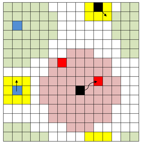
Figure 1. Sketch of the model. Currently quiescent (active) citizens are represented by blue (red) cells, LEOs are represented by black cells. Yellow cells show Moore neighborhood for an agent. During a move, an agent picks a random cell in his/her neighborhood and if the selected cell is unoccupied, he/she moves there, otherwise the agent stays put. Pink cells show a vision of radius 4 for the LEO (black cell). The LEO arrests the nearest active citizen in its field of vision. Green cells show vision of radius 4 for the citizen (blue cell). The citizens calculate their state depending on conditions on the lattice within their field of vision. - 3.2
- The agent-based model described in (Epstein 2002) was used as a starting point in developing the model described below. Each citizen is assigned the hardship H drawn from the uniform distribution U(0,1). The hardship is heterogeneous across citizens, but constant for any one citizen. The perceived legitimacy L of the law enforcement authority is equal across citizens and can be between 0 and 1. The hardship and the legitimacy are used to define citizen’s grievance E = H(1-L). The citizen's grievance decreases with the increase of the legitimacy. If legitimacy is high, then even big hardship does not produce grievance. If hardship is high, then low legitimacy can produce high grievance.
- 3.3
- Some citizens are more willing to pursue criminal activity than others, encoded by the risk aversion K. Each individual’s risk aversion is drawn from U(0,1) and is constant for each citizen. The citizen’s vision v is a circle of radius v that comprises lattice positions that the citizen is able to inspect. It is equal across citizens. The citizen’s perceived net risk N is defined as follows: N = KP, where P is a function of the ratio of LEOs to active citizens in the citizen's vision.
- 3.4
- In contrast to (Epstein
2002; Epstein 2006),
in our model the net perceived risk of a citizen does not increase
monotonically with the local ratio of LEOs to active citizens. In one of the
two functional forms we use, perceived risk is zero up to a threshold value,
after which it increases monotonically (see Fig. 2), thus giving
sigmoidal shape. The sigmoidal functional form encodes a level of irrational
behavior by citizens, where the perceived risk of being incarcerated is
diminished by the proportion of others locally observed to be in the same
situation. Law enforcement operates through the rule that a LEO agent arrests
the nearest active citizen, randomly choosing among citizens if there are two
or more that are equally close by. This rule leads to dynamics in which local
crime hotspots attract police action, thus reflecting modern problem-oriented
policing law enforcement strategies (Braga
2008). For comparison, in Fig. 2 we show a
monotonically increasing curve, representing “rational” behavior.
This type of functional form does not lead to good fit with data. The linear dependence of the citizen's
perceived risk on the the LEOs-to-actives ratio also does not lead to good
comparison with data.

Figure 2. Citizen’s perceived risk functions depending on the ratio x of the number of LEOs to the number of active citizens in the citizen’s vision. The “rational” function corresponds to the case when citizen’s perceived risk increases monotonically with x. - 3.5
- The citizen’s perceived risk function P of type “step” is defined as:
while function P of “sigmoidal” type is defined as:
and function P of type “rational” is defined as:
and function P of type “linear” is defined as:
where A is the number of active citizens (including self) within citizen’s vision, C is the number of LEOs within citizen’s vision, constant k = 9.2104 is found from the condition that P (1/4) = 0.9, constant k ′ = 62.6716 is found from the condition that P(1/4) = 0.5. Value 0.9 for the perceived risk is considered to be a plausible estimate for the situation. The citizen’s perceived risk function P of type step (red curve in Fig. 2) is chosen to be zero up to the value of 0.9 of the rational curve (black curve in Fig. 2) what gives us the point of LEOs-to-actives ratio equal to 1/4. The citizen’s perceived risk function P of sigmoidal type (blue curve in Fig. 2) is a smoothed version of the step function and is equal to 0.5 at the center, i.e. P (1/4) = 0.5.
- 3.6
- For a law-abiding citizen, if the difference E - N exceeds T, where T is some threshold, then the citizen becomes criminally active. For an active citizen, if the difference E - N exceeds T, then the citizen stays active. Otherwise, he/she becomes law-abiding. In summary, the citizen’s rule for being active or quiescent is the following: If E -N > T be active; otherwise, be quiescent. The LEO’s vision w is a circle of radius w that comprises lattice positions that the LEO is able to inspect. It is equal across LEOs. The LEO’s rule is the following: Inspect all sites within w and arrest the nearest active citizen. Jail terms for arrested actives are assigned randomly from U(0,Jmax), where Jmax is the maximum jail term. Citizens and LEOs move on the lattice by using the following movement rule: Pick a random neighboring location on the lattice (from Moore neighborhood), if that location is unoccupied - move there, if the location is occupied - stay put.
- 3.7
- A citizen’s state is a function of hardship and risk
aversion which differ for each individual citizen as well as the perceived
legitimacy of the authority (L), which is constant across all
citizens. Citizens become active or quiescent depending on their perceived
risk, which changes based on local conditions within the field of vision of a
citizen (Fig. 2). In
general, citizens are less likely to engage in violence as the local ratio
between number of LEOs and active citizens increases, due to the fear of being
identified and incarcerated. A threshold value T determines the
situation in which all citizens are inactive. In particular, in the case where
T > 1 - L, all citizens are always quiescent regardless of the
lattice situation; we call these citizens “never active” and denote
their fraction in the population as G. In the case where T <
-1, all citizens are “always active”, and we denote their
fraction in the population as R. When -1 < T < 0, G
= 0, all citizens are either “always active” or
“conditionally active” (active or quiescent depending on the
lattice situation). The case where 0 < T < 1 - L is the most
realistic in that all three types of citizen present in the population. In
practice, the threshold T and legitimacy L for the model run
can be found using statistical data on R and G in the
population:

(1) 
(2) - 3.8
- The procedure of a run is the following. A citizen or a LEO is selected at random. The probability of selecting a LEO is higher according to the number of moves a LEO can make per day. If the selected person is a non-jailed citizen, then he/she moves according to the movement rule; if the citizen is in jail, then the days at jail are calculated and if the number of days at jail is equal to the assigned jail term the released citizen is put on a random unoccupied site on the lattice. After that the state of the citizen is calculated depending on the current lattice situation. If the selected person is a LEO, then he/she inspects all sites within the vision, arrests the nearest active citizen (if any) and jumps to the location of the arrested by him citizen. The jailed citizens are placed outside the lattice. Then the LEO moves under the movement rule. The pseudocode for the simulation can be found in the Appendix. The model iterates this procedure until the simulation time is reached. Some simulations of the model can be seen at the web-site Model simulations.
Number of LEO's and Tipping Points as a Function of City Size
- 4.1
- In the following we compare the results of our model of crime and violence in cities with FBI data[1], [2]on violent crimes in 5,660 U.S. cities over the period of 2005–2009. For comparison with the statistical data we assume that one “citizen agent” in our model represents Ac = 9 real citizens. Our model is then used to understand the origin of violent crime in cities with different population sizes. Tipping points for communities of all sizes are observed in the model: reducing the number of LEOs below a critical level rapidly increases the incidence of criminal/violent activity. The results obtained using step and sigmoidal types of net perceived risk functions are very similar and demonstrate the robustness of the model. For both step and sigmoidal types the net perceived risk is zero for small ratios of LEOs to actives, while it's not zero for the “rational” and linear types. Dependences with zero risk for small LEO-to-actives ratios give similar results what proves the robustness of the model. As expected, when the number of LEOs in a city is increased, the number of active citizens decreases. In a surprising outcome of the modeling, we observe that for cities with larger population, the fraction of LEOs in a city has to be increased in order to keep the same level of activity of citizens.
- 4.2
- Figure 3 shows the dependence of the number of active citizens per day (in
percent) on the number of LEOs per 1,000 citizens for citizen’s perceived
risk functions of sigmoidal type (blue solid line), step type (red dashed line)
and linear type (green solid line). Six lattices sizes (100x100, 200x200,
300x300, 400x400, 500x500, 600x600) were considered with the corresponding real
population of 63,000; 252,000; 567,000; 1,008,000; 1,575,000; 2,268,000.
We consider that citizen density is 0.7*Ac; citizen vision is 14; LEO
vision is 14; LEO speed is 4 (i.e. LEOs move 4 times per day); maximum jail
term is 120 days; fraction of “always active” citizens R = 0.025; fraction of “never active”
citizens G = 0.5; fraction of
“conditionally active” citizens is 0.475. Threshold T and legitimacy L can be
calculated by using formulas (1) and (2), respectively, and are
as follows: T = 0.1, L = 0.8. The chosen parameters describe the typical city. All
“always active” citizens are initially in jail. 1,000 days on the
lattice were computed for each simulation. Each experiment was repeated at
least 80 times. The model was implemented in Visual Studio C++ with the GUI
graphical interface. The validation of the model will be presented later in the
paper. Parameter ranges for the number of LEOs per 1,000
citizens are chosen to encompass those observed in real-world setting[3]. The number of active
citizens is unconstrained, but always represents a small fraction of the total
population at any one time. For example, the City of Los Angeles is estimated
to have nearly 40,000 gang members and a total population of approximately 4
million, representing at most 1% of the population. Only a fraction of these
gang members are actively engaged in crime at any moment in time. It is easy to see that for the larger lattices (the
cities with larger population), the fraction of LEOs in a city has to be
increased in order to keep the same level of activity of citizens.
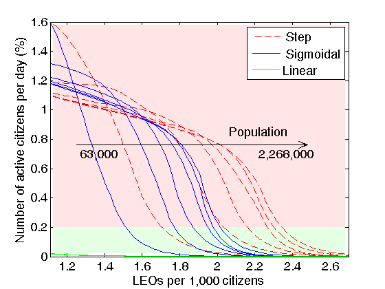
Figure 3. Dependence of the number of active citizens per day (in percent) on the number of LEOs per 1,000 citizens for population corresponding to lattices from 100x100 to 600x600 (real population sizes from 63,000 to 2,268,000) for citizen’s perceived risk functions of sigmoidal type (blue solid line), step type (red dashed line) and linear type (green solid line). Six lines of each type correspond to populations 63,000; 252,000; 567,000; 1,008,000; 1,575,000; 2,268,000, from left to right, respectively. The values of the number of active citizens per day (in percent) for the linear perceived risk function are decreasing from 0.0181% for 1.1 LEOs per 1,000 citizens to 0.001% for 2.7 LEOs per 1,000 citizens for the lattice size of 100x100 and from 0.0223% for 1.1 LEOs per 1,000 citizens to 0.0011% for 2.7 LEOs per 1,000 citizens for the lattice size of 600x600. Other model parameters are as follows: citizen density is 0.7*Ac; citizen vision is 14; LEO vision is 14; LEO speed is 4; maximum jail term is 120 days; fraction of “always active” citizens R = 0.025; fraction of “never active” citizens G = 0.5; fraction of “conditionally active” citizens is 0.475. The plot represents simulation results. - 4.3
- Figure 4
shows the dependence of the number of LEOs per 1,000
citizens on population needed to keep a below-threshold fixed level of
violent and/or criminal activity of citizens. 0.2% level
of active citizens per day is considered an acceptable level. All
parameter settings are the same as for Fig. 3. For both
step and sigmoidal net perceived risk functional dependencies, the ratio of
LEOs in the population increases logarithmically with the population size. The
same situation is observed in the real life what is suggested by the
International Association of Chiefs of Police[3].
It can be also seen that the number of LEOs per 1,000 citizens needed to
maintain a certain level of activity is a decelerating function of the
population size. This suggests that growth from small cities to medium cities
requires a much greater increase in the relative density of LEOs to citizens
compared with growth from medium to large cities.
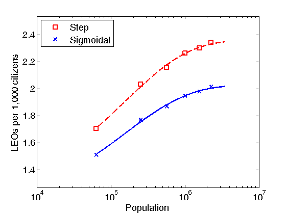
Figure 4. Dependence of the number of LEOs per 1,000 citizens on the population size needed to keep a 0.2% level of active citizens per day for citizen’s perceived risk functions of sigmoidal type (blue line) and step type (red line). All model parameters are the same as for Fig. 3. The plot represents simulation results. - 4.4
- To understand the robustness of the obtained results as well
as stochastic nature of the agent-based model we generate 10,000 samples in the
3-dimensional space of citizen density, number of LEOs per 1,000 citizens, and
population size. For each sample, the model is evaluated and then an analytical
model is learned based on all samples (support vector regression is used for
learning). Citizen density was drawn from the uniform distribution on
Ac*[0.2;0.8], number of LEOs per 1,000 citizens was
drawn from the uniform distribution on [0.55;3.89], population size was drawn
from the uniform distribution on [9000; 900000]. The other parameters are as
following: LEO speed is 5, maximum jail term is 175 days, “always
actives” fraction is 0.025, “never actives” fraction is 0.45,
“conditionally active” fraction is
0.525. The number of the nearest neighbors Nc for each citizen is fixed
and is equal to 2124 citizens (236 agents). The citizen vision is calculated as
follows:
 . LEO
vision is equal to citizen vision. The lattice size is calculated as follows:
. LEO
vision is equal to citizen vision. The lattice size is calculated as follows:
 . All
“always active” citizens are initially in jail. The sigmoidal type
of the risk perception function was used. 2,000 days on the lattice were
computed for each simulation. In the case of the fixed population and the fixed
number of the nearest neighbors for each citizen, the parameter defining
citizen density can be considered the agent daily relative diffusivity. The
small diffusivity corresponds to small diffusion of LEOs per day, the big
diffusivity corresponds to large diffusion of LEOs per day. The agent daily
relative diffusivity is inversely proportional to the lattice area.
. All
“always active” citizens are initially in jail. The sigmoidal type
of the risk perception function was used. 2,000 days on the lattice were
computed for each simulation. In the case of the fixed population and the fixed
number of the nearest neighbors for each citizen, the parameter defining
citizen density can be considered the agent daily relative diffusivity. The
small diffusivity corresponds to small diffusion of LEOs per day, the big
diffusivity corresponds to large diffusion of LEOs per day. The agent daily
relative diffusivity is inversely proportional to the lattice area.
- 4.5
- In the following we define the rate of
violence as the average number of citizens active at the end of the day or
jailed during the day per 1,000 citizens. The difference between the rate of
violence and the number of active citizens per day (in
percent) is that the number of citizens jailed during the day is also included
in the rate of violence. In Fig. 5 the
dependence of the rate of violence on the number of LEOs
per 1,000 citizens is presented. It can be seen not only that the effect
of the number of LEOs per 1,000 citizens on the
rate of violence is non-linear, within a population of fixed size and fixed
citizen density, but also that a higher number of LEOs
per 1,000 citizens is needed for larger populations to maintain the same
rate of violence. The 2.3 LEOs per 1,000 citizens
is the tipping point for this set of parameters. When the number of LEOs per
1,000 citizens is bigger than 2.3, the rate of
violence is very small, citizens stay quiescent because of the high probability
to be arrested. For the number of LEOs per 1,000
citizens less than 2.3 and bigger than 1.9, there is a sharp increase in
the rate of violence, which slows down for the number of LEOs per 1,000 citizens from 1.4 to 1.9. For the number of LEOs
per 1,000 citizens from 1.4 to 1.9 the activity
somewhat stabilizes because a lot of population is in the jail. For the number
of LEOs per 1,000 citizens less than 1.4 the jail
can no longer contain all actives and the rate of violence starts to
increase.
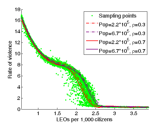
Figure 5. Dependence of the rate of violence on the number of LEOs per 1,000 citizens. Green points represent 10,000 sampling points. Fitting lines are shown for population of 2.2 * 105 and 6.7 * 105 citizens and citizen density of 0.3*Ac and 0.7*Ac. Model parameters are as follows: citizen density was drawn from the uniform distribution on Ac*[0.2;0.8], number of LEOs per 1,000 citizens was drawn from the uniform distribution on [0.55;3.89], population size was drawn from the uniform distribution on [9000; 900000], LEO speed is 5, maximum jail term is 175 days, “always actives” fraction is 0.025, “never actives” fraction is 0.45, “conditionally active” fraction is 0.525. The number of the nearest neighbors Nc for each citizen is fixed and is equal to 2124 citizens. The citizen vision is calculated as follows: . LEO vision is equal to citizen
vision. The plot represents simulation results. - 4.6
- Figure 6
conveys a similar situation. Shown is the dependence of the number of LEOs per
1,000 citizens on population size and on rate of violence. In this case number of LEOs per 1,000 citizens was drawn from the uniform
distribution on [1.67;2.78], population size was drawn from the uniform
distribution on [9000; 3600000]. All other parameters are the same as
for Fig. 5. The black dashed line represents a rate of
violence equal to 2. To keep the same rate of violence for different population
sizes, the number of LEOs per 1,000 citizens has
to increase super-linearly with the increase in population.
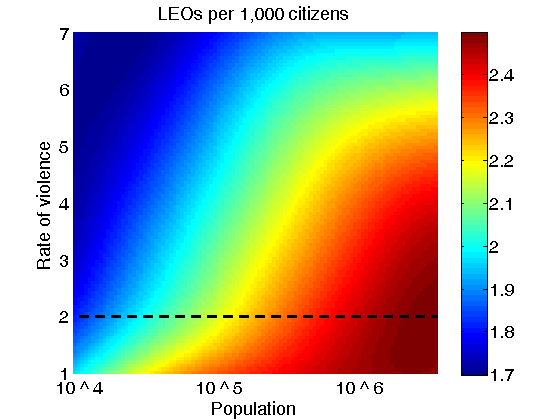
Figure 6. Dependence of the number of LEOs per 1,000 citizens on the population size and the rate of violence. The number of LEOs per 1,000 citizens was drawn from the uniform distribution on [1.67;2.78], population size was drawn from the uniform distribution on [9000; 3600000]. All other parameters are the same as for Fig. 5. The plot represents simulation results. - 4.7
- Figure 7
shows a smooth fit of FBI data on the number of LEOs per 1,000 citizens as a
function of violent crime rate and population size. White
dots represent 5,660 U.S. cities. The color bar to the right indicates
the number of LEOs per 1,000 citizens that corresponds to the color band where
the specific white dot is plotted. The number of LEOs per 1,000 citizens for
experimental data is not displayed here because of the data being noisy. Only
the value of the smooth fit is displayed. As our model predicts, the fraction
of LEOs in the U.S. cities increases with population. Having established this
fact, we assume in the following that the number of LEOs in cities is chosen to
keep the same low level of violent activity of citizens. This means that we
will use the number of LEOs per 1,000 citizens
from Fig. 4 when varying the
size of the lattice. The assumption that the number of
LEOs per 1,000 citizens is chosen in such a way to keep below 0.2% level
of violent activity makes our model consistent with the FBI data and makes our
model very robust with respect to all model parameters.
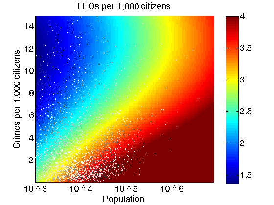
Figure 7. The number of LEOs per 1,000 citizens as a function of the number of violent crimes per 1,000 citizens and the population size. The plot is a smooth fit of FBI data. White dots represent 5,660 U.S. cities. The color bar to the right indicates the number of LEOs per 1,000 citizens that corresponds to the color band where the specific white dot is plotted.
Spatial-Temporal Structure of Large-Scale Outbursts
- 5.1
- To understand how violent outbursts might emerge in cities
with different population sizes, we compare the temporal and spatial
distribution of violent/criminal activity in simulations on small and large
lattices. Such spatio-temporal properties have recently attracted quite a bit
of attention in crime research (Ratcliffe 2004). As seen in Fig. 8A, violent outbursts happen
more frequently in the large city, but the fraction of the population
participating in the outburst is significantly smaller. Figures 8B and 8C show three snapshots
(before, during, and after the peak of activity) for the lattices representing
small and large cities, respectively. The entire population capable of going
active (blue points), does so (red points) during a violent outburst in a small
city (Fig. 8B). The
picture is completely different for a large city (Fig. 8C). Here only a fraction of
the population goes active during the peak of the spatio-temporal crime
hotspot. When the outburst is suppressed by LEOs on a large lattice, a large
fraction of the population is not even aware that an outburst took place.
Growth of crime/violence hotspots is caused by inhomogeneity in the spatial
distribution of citizens and LEOs. In particular, it can be seen in Figures 8B and 8C that LEOs (black points)
chase criminals and form dense clusters in the process of suppressing a
hotspot. The resulting inhomogeneity in the LEO distribution creates areas with
almost no LEOs, which locally reduces citizens' net perceived risk and drives
new violent outbursts (see Fig. 2). Not every outburst
generated in this way is large-scale, however. In the following we introduce a
threshold (e.g. 5% of population) and call an outburst large-scale if it
exceeds the threshold. Note that no such outbursts are observed when the
perceived risk depends monotonically on local ratio of LEOs to active citizens;
the “rational” dependence shown in Fig. 2. Thus, the
spatio-temporal hotspots are, in the model, partially due to
“irrationality” in citizen behavior: starting from a threshold
value of the number of their neighbors that are active, citizens do not care if
they get arrested. The police force reacts to a local outburst, but that makes
the situation worse, since it depletes policing levels nearby and thus triggers
growth in the spatio-temporal hotspot. In a larger city, at constant population
density, the fact LEOs end up chasing crime hotspots, leaving some areas
under-policed, necessitates an increased LEO/citizen ratio to maintain a
constant low crime rate.
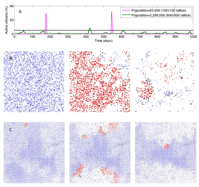
Figure 8. A) The number of active citizens (in percent) as a function of time for 100x100 and 600x600 lattices. Horizontal dashed line shows 5% threshold for large-scale outbursts. The sigmoidal type of the citizen’s perceived risk function is used. Model parameters are as follows: citizen density is 0.7*Ac; citizen vision is 14; LEO vision is 14; LEO speed is 4; maximum jail term is 120 days; fraction of “always active” citizens R = 0.025; fraction of “never active” citizens G = 0.5; fraction of “conditionally active” citizens is 0.475. Number of LEOs per 1,000 citizens for each case is taken from Fig. 4 and is equal to 1.51 and 2.02 for lattices of size 100x100 and 600x600, respectively. B) The lattice situation at day 540 (left pane), at day 545 (middle pane) and at day 550 (right pane) for the lattice of size 100x100. Red points represent active citizens; blue points represent quiescent citizens who can become active; black points represent LEOs, empty cells represent non-occupied places and “never active” citizens. C) The lattice situation at day 893 (left pane), at day 905 (middle pane) and at day 917 (right pane) for the lattice of size 600x600. The plot represents simulation results.
Crime Trends and Violence in Cities
- 6.1
- Figure 9 shows a smooth fit of FBI
data on a yearly number of violent crimes per 1,000 citizens in the U.S. cities
for period 2005–2009 as a function of the population size. Murder and non-negligent manslaughter, forcible rape, robbery, and
aggravated assault are considered a violent crime. Blue dots represent 5,660 U.S. cities. As seen from
Fig. 9 the number of
violent crimes per 1,000 citizens increases with population and then starts to
stabilize. In the following we show that this is because of strong dependence
of the number of violent outbursts on the number of LEOs
per 1,000 citizens in cities with large population. Number of crimes per 1,000 citizens is
proportional to population size to the power of 0.1678, which can be calculated
as the slope of the green line in the small plot in log scale in Fig. 9.
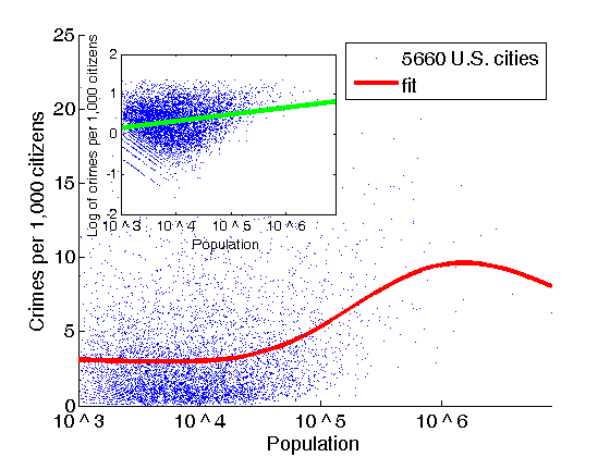
Figure 9. The number of crimes per 1,000 citizens as a function of the population size. The plot is a smooth fit of FBI data. Blue dots represent 5,660 U.S. cities. - 6.2
- To provide an explanation for the peculiar dependence on
cities’ population, we will look at the population dependence of the
number of violent outbursts in our model. We define the number of violent
outbursts per year to be inversely proportional to the waiting time between two
large-scale outbursts. Figure 10 shows an
analytical fit for the number of violent outbursts per year. Parameters of the
model are the same as those for Fig. 6. With the smart selection of
the number of LEOs per 1,000
citizens (white dotted curve) the situation is stable even in very large
cities. When the average number of
LEOs per 1,000 citizens is used (black dashed line) the situation can
become unstable for very large cities what is observed in the real data.
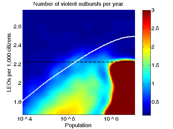
Figure 10. Dependence of the number of violent outbursts per year on the population and the number of LEOs per 1,000 citizens. All model parameters are the same as for Fig. 6. The plot represents simulation results. - 6.3
- We see from Fig. 11 that for the fixed number of
LEOs per 1,000 citizens the rate of violence increases significantly with
population. With the smart selection of the number of
LEOs per 1,000 citizens the rate of violence is, indeed, the highest for
intermediate lattice sizes. This phenomenon does not depend on the perceived
net risk function (Fig. 2), as long as it is
sigmoidal.
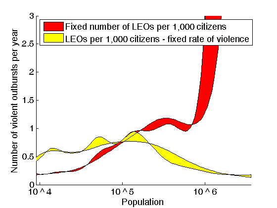
Figure 11. Number of violent outbursts per year in dependence on the population size. Band shows variation in outburst threshold from 4% to 5%. All model parameters are the same as for Fig. 6. The plot represents simulation results. - 6.4
- Why are the mid-sized cities more prone to violence? In
Fig. 8 we saw that the
outbursts of activity become more frequent, but more localized as the size of
the lattice increases. At the same time, the peak number of active citizens
decreases with the lattice size (Fig. 12). Since the police
force is instructed to keep the overall frequency of violent events below a
threshold the number of violent outbursts starts to decrease with lattice size
for large lattices.
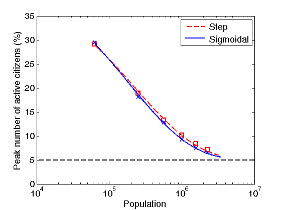
Figure 12. Dependence of the number of active citizens (in percent) at the peak of the violent outburst on the population. All model parameters are the same as for Fig. 3. The plot represents simulation results. - 6.5
- In our model, a citizen's vision reflects both the level of
information he/she possesses as well as population density. The level of
information is linked to the average number of neighbors for each citizen. The
number of neighbors can be calculated by using the following formula:
 . If citizens have the same level
of information for different population densities, then the citizen vision is
inversely proportional to the square root of population density. Fig. 13 shows the
dependence of the rate of violence on the citizen vision (LEO vision is fixed).
The rate of violence is lowest when citizen vision is slightly less than
LEO’s vision. When citizen vision becomes very small or when it is
approximately equal to LEO’s vision, the rate of violence rapidly
increases. The increase in violence with small vision can be called as an
"ignorance of risk" effect, while the increase in violence when citizen vision
is greater than LEO vision can be called as a "bravado" effect. In view of
this, the rate of violent crimes could be reduced in cities with small
population density by increasing the awareness of LEO presence while in cities
with large population density, information level of LEOs has to be increased
appropriately, so that they can anticipate and respond to the next violent
outburst will occur.
. If citizens have the same level
of information for different population densities, then the citizen vision is
inversely proportional to the square root of population density. Fig. 13 shows the
dependence of the rate of violence on the citizen vision (LEO vision is fixed).
The rate of violence is lowest when citizen vision is slightly less than
LEO’s vision. When citizen vision becomes very small or when it is
approximately equal to LEO’s vision, the rate of violence rapidly
increases. The increase in violence with small vision can be called as an
"ignorance of risk" effect, while the increase in violence when citizen vision
is greater than LEO vision can be called as a "bravado" effect. In view of
this, the rate of violent crimes could be reduced in cities with small
population density by increasing the awareness of LEO presence while in cities
with large population density, information level of LEOs has to be increased
appropriately, so that they can anticipate and respond to the next violent
outburst will occur.
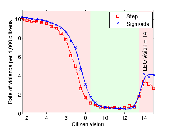
Figure 13. The rate of violence per 1,000 citizens as a function of the citizen vision for population of 567,000. The dependence on citizen vision is very similar for all population sizes. Model parameters are as follows: citizen density is 0.7*Ac; LEO speed is 4; maximum jail term is 120 days; fraction of “always active” citizens is 0.025; fraction of “never active” citizens is 0.5; fraction of “conditionally active” citizens is 0.475. Number of LEOs per 1,000 citizens is taken from Fig. 4 for lattice size of 300x300 and is equal to 1.87. The plot represents simulation results.
Conclusions
- 7.1
- In this paper we have used dynamically evolving agent-based modeling to study dependence of the frequency of violence and criminal activity on population size. We have presented FBI data on violent crime in 5,660 U.S. cities over the period 2005–2009. We compare these data to the outputs of our model, finding good agreement. The obtained results indicate that observed large-scale trends, such as an increased proportion of police to population in large cities can be attributed to partially irrational behavior of citizens in hotspot areas, which fuels further growth of spatio-temporal patterns of crime. In addition, the model indicates that for all sizes of communities studied here, there are tipping points: LEO to citizen ratios below which violent and criminal activity rapidly increases. We clarify that the primary mechanism responsible for increasing proportion to police relative to population is not the irrational behavior of citizens, but rather the fact that police cannot simultaneously suppress eruptions of violence in multiple places, even though they are cognizant of multiple conflagrations. Police face an opportunity in larger systems where they have to choose which battles to fight. It is encouraging that simple models of the sort described here can help explain puzzling trends in data, and we hope that much more sophisticated agent-based models that include geography, transportation and social capital could be devised to give an even higher level of predictability. A next step in our research would be to examine the general predictions of the model at a finer spatio-temporal scale. Does the model provide a good description of police resource allocation problems in a single, diverse city like Los Angeles, Chicago or New York?
Appendix: Model Simulation Pseudo Code
-
place agents on the lattice

set up characteristics for all citizens

place “always active” citizens in the jail

for each time step
{
	for each agent (note that a LEO can move several times per day and is accessed several times)
	{
		an agent (citizen or LEO) is selected

		if the agent is a citizen
		{
			if the citizen is not in the jail
			{
				the citizen moves
			}
			else
			{
				the remained jail term is calculated and if the jail term is over the citizen
				is released and put on a random unoccupied site on the lattice
			}

			the state of the non-jailed citizen is calculated
		}

		if the agent is a LEO
		{
			the LEO arrests a nearest active citizen (if any) within the vision
			and jumps to the location of the arrested by him citizen

			the LEO moves
		}
	}

	the number of active and jailed citizens is calculated
}
Acknowledgements
- This work was partially supported by AFOSR Grant FA9550-08-1-0217. We are grateful to the editor and anonymous referees for their helpful comments and suggestions.
Notes
-
1 FULL-TIME LAW ENFORCEMENT EMPLOYEES BY STATE
BY CITY Federal Bureau of Investigation (www.fbi.gov/ucr/05cius/data/table_78.html,
www.fbi.gov/ucr/cius2006/data/table_78.html,
www.fbi.gov/ucr/cius2007/data/table_78.html,
www.fbi.gov/ucr/cius2008/data/table_78.html)
2 OFFENSES KNOWN TO LAW ENFORCEMENT BY STATE BY CITY Federal Bureau of Investigation (www.fbi.gov/ucr/05cius/data/table_08.html, www.fbi.gov/ucr/cius2006/data/table_08.html, www.fbi.gov/ucr/cius2007/data/table_08.html, www.fbi.gov/ucr/cius2008/data/table_08.html)
3 POLICE OFFICER TO POPULATION RATIOS, The International Association of Chiefs of Police, 2007 (http://www.theiacp.org/PublicationsGuides/ContentbyTopic/tabid/216/Default.aspx?id=1051&v=1)
References
-
AGNEW R (1992) Foundation for a general strain theory of crime and delinquency. Criminology 30(1). pp. 47–88. [doi:10.1111/j.1745-9125.1992.tb01093.x]
AGNEW R (2001) Building on the foundation of general strain theory: Specifying the types of strain most likely to lead to crime and delinquency. Journal of Research in Crime and Delinquency 38(4). p. 319. [doi:10.1177/0022427801038004001]
BETTENCOURT L M A, Lobo J, Strumsky D, West G B (2010) Urban Scaling and Its Deviations: Revealing the Structure of Wealth, Innovation and Crime across Cities. PLoS ONE 5(11): e13541. [doi:10.1371/journal.pone.0013541]
BINGENHEIMER J B, Brennan R T, Earls F J (2005) Firearm violence exposure and serious violent behaviour. Science 308. pp. 1323–1326. [doi:10.1126/science.1110096]
BLOCK R, GALARY A, BRICE D (2007) The Journey to Crime: Victims and Offenders Converge in Violent Index Offences in Chicago. Security Journal 20, pp. 123–137. [doi:10.1057/palgrave.sj.8350030]
BOSSE T, Gerritsen C (2010) Social Simulation and Analysis of the Dynamics of Criminal Hot Spots. Journal of Artificial Societies and Social Simulation 13 (2) 5 https://www.jasss.org/13/2/5.html
BRAGA A A (2008) Problem-oriented policing and crime prevention. Criminal Justice Press.
CLARKE R (1995) Situational Crime Prevention. In Building a Safer Society: Strategic Approaches to Crime Prevention, edited by M. Tonry and D. Farrington. Chicago: University of Chicago Press. [doi:10.1086/449230]
COHEN L. E., Felson M. (1979) Social-Change And Crime Rate Trends - Routine Activity Approach. American Sociological Review 44, pp. 588–608. [doi:10.2307/2094589]
ECK J E, Chainey S, Cameron J G, Leitner M, Wilson R E (2005) Mapping Crime: Understanding Hot Spots. National Institute of Justice Special Report (www.ncjrs.gov/pdffiles1/nij/209393.pdf).
EPSTEIN J M (2002) Modeling civil violence; an agent-based computational approach. Proc. Natl. Acad. Sci. USA 99. pp. 7243–7250. [doi:10.1073/pnas.092080199]
EPSTEIN J M (2006) Generative Social Science: Studies in Agent-Based Computational Modeling. Princeton University Press, Princeton, NJ.
FELSON M, Clarke R V (1998) Opportunity Makes the Thief: Practical Theory for Crime Prevention. Home Office Policing and Reducing Crime Unit, London.
GALULA D (1964) Counterinsurgency Warfare: Theory and Practice. Praeger Security International. Westport, CT.
GOTTFREDSON M R, Hirschi T (1990) A General Theory of Crime. Stanford: Stanford University Press.
GROFF E (2007) Simulation for Theory Testing and Experimentation: An Example Using Routine Activity Theory and Street Robbery. Journal of Quantitative Criminology 23. pp. 75–103. [doi:10.1007/s10940-006-9021-z]
JACOBS B A, Wright R (2006) Street justice: Retaliation in the criminal underworld. Cambridge University Press.
KILCULLEN D (2009) The Accidental Guerrilla: Fighting Small Wars in the Midst of a Big One. Oxford University Press. Oxford.
LIM M, Metzler R, Bar-Yam Y (2007) Global pattern formation and ethnic/cultural violence. Science 317. pp. 1540–1544. [doi:10.1126/science.1142734]
LIU L, Eck J (2008) Artificial crime analysis systems: using computer simulations and geographic information systems. Information Science Reference. [doi:10.4018/978-1-59904-591-7]
MAKOWSKY M (2006) An Agent-Based Model of Mortality Shocks, Intergenerational Effects, and Urban Crime. Journal of Artificial Societies and Social Simulation 9(2) 7 https://www.jasss.org/9/2/7.html
MALLESON N, Brantingham P (2009) Prototype burglary simulations for crime reduction and forecasting. Crime patterns and analysis 2(1). pp. 47–66
MURPHY K, Hinds L, Fleming J (2008) Encouraging public cooperation and support for police. Policing and Society 18(2). pp. 136–155. [doi:10.1080/10439460802008660]
PRATT T C, Cullen F T (2000) The Empirical Status of Gottfredson and Hirschi's General Theory of Crime: A Meta-analysis. Criminology 38. pp. 931–964. [doi:10.1111/j.1745-9125.2000.tb00911.x]
RATCLIFFE J (2004) The Hotspot Matrix: A framework for the spatio-temporal targeting of crime reduction. Police Practice and Research 5. pp. 5–23. [doi:10.1080/1561426042000191305]
RATCLIFFE J (2008) Intelligence-Led Policing. Willan, Portland.
RAUHUT H, Junker M (2009) Punishment Deters Crime Because Humans Are Bounded in Their Strategic Decision-Making. Journal of Artificial Societies and Social Simulation 12 (3) 1 https://www.jasss.org/12/3/1.html
RENGERT G F, Piquero A R, Jones P R (1999) Distance decay reexamined. Criminology 37. pp. 427–445. [doi:10.1111/j.1745-9125.1999.tb00492.x]
ROSSMO D K (2000) Geographic Profiling. CRC Press, Boca Raton.
SAMPSON R J, Raudenbush S W, Earls F (1997) Neighbourhoods and violent crime: a multilevel study of collective efficacy. Science 277. pp. 918–924. [doi:10.1126/science.277.5328.918]
SHORT M B, D’OrsognA M R, Pasour V B, Tita G E, Brantingham P J, Bertozzi A L, Chayes L B (2008) A statistical model of criminal behaviour. Mathematical Models and Methods in Applied Sciences 18. pp. 1249–1267. [doi:10.1142/S0218202508003029]
TITA G, Griffiths E (2005) Traveling to Violence: The Case for a Mobility-Based Spatial Typology of Homicide. Journal of Research in Crime and Delinquency 42(3). pp. 275–308. [doi:10.1177/0022427804270051]
TITA G, Ridgeway G (2007) The Impact of Gang Formation on Local Patterns of Crime. Journal of Research in Crime and Delinquency 44. pp. 208–237. [doi:10.1177/0022427806298356]
WILSON M, Daly M (1985) Competitiveness, risk taking, and violence: The young male syndrome. Etiology and Sociobiology 6. pp. 59–73. [doi:10.1016/0162-3095(85)90041-X]