
 Abstract
- This paper documents our efforts (and troubles) in replicating Epstein's (1998) demographic prisoner's dilemma model. Confronted with a number of ambiguous descriptions of model features we introduce a method for systematically generating a large number of model replications and testing for their equivalence to the original model. While, qualitatively speaking, a number of our replicated models resemble the results of the original model reasonably well, statistical testing reveals that in quantitative terms our endeavor was only partially successful. This fact hints towards some unstated assumptions regarding the original model. Finally we conduct a number of statistical tests with respect to the influence of certain design choices like the method of updating, the timing of events and the randomization of the activation order. The results of these tests highlight the importance of an explicit documentation of design choices and especially of the timing of events. A central lesson learned from this exercise is that the power of statistical replication analysis is to a large degree determined by the available data.
- Keywords:
- Agent-Based Model, Verification, Comparative Computational Methodology, Prisoners Dilemma, Replication, Demographic Prisoners Dilemma
Introduction
- 1.1
- Although agent-based models are clearly on the rise as a modeling tool, the replication (and therefore verification) of such models has long been regarded "as an activity for students learning about social simulation, rather than something for innovative professors to trouble themselves with" (Rouchier et al. 2008). As Edmonds and Hales (2003) trenchantly remarked "an unreplicated simulation is an untrustworthy simulation" which of course is not a statement of the bad intentions of modelers but simply documents the vast possibilities for errors and artefacts that might have been introduced in the process of creating the model in the first place (Galan et al. 2009), errors and artefacts the model creators themselves are not aware of. Therefore neglecting the importance of replications is a rather unsatisfactory state of affairs.
- 1.2
- Fortunately, replication, along with other techniques used for model-to-model analysis, is gaining currency, not at least due to the impact of dedicated workshops trying to advance this set of methods (Hales et al. 2003; Rouchier et al. 2008). Accompanied by such initiatives there has also been a marked rise in the number of publications dealing with replication. What most of them have in common is that, beside the main goal of verifying the model-to-be-replicated, a number of valuable insights on the method of ABM have been gained.
- 1.3
- Edmonds and Hales (2003), for instance, derived from their experiences with replication the need for a norm concerning the publication of simulation results, i.e. a sufficiently detailed description of the original model in order for others to be replicable. Furthermore they illustrated the potential gains of re-implementing a model in two different simulation frameworks. Edmonds and Hales (2005) show how replication can help clarify the scope of existing models' results, i.e. demonstrating that some results thought to be generally true are only valid for special cases, or on the contrary, that some results hold true beyond the scope investigated by the original author. Bigbee et al. (2007) utilize a replication attempt to test the capabilities of a simulation framework with the aim of possibly further improving the framework.
- 1.4
- Galan and Izquierdo (2005) illustrated the benefit of complementing simulations with analytical work, a thread later picked up by Izquierdo et al. (2009) who demonstrate the former insight impressively by extensive use of Markov Chain analysis. The efforts of Rouchier (2003) show that even in the case of close communication with the original model author, the results of the original model may not be replicable, which points out the difficulties of communicating a conceptual model. At times, differences between the original model and the replicated one can only be resolved after extensive scrutiny of the original model's source code (Will and Hegselmann 2008; Will 2009).
- 1.5
- The present article is related to the above mentioned replication efforts but tries to advance the use of statistical testing for the evaluation of replication success. Thus, it is closely related to and tries to extend insights from Edmonds and Hales (2003) as well as Wilensky and Rand (2007). Facing several ambiguous descriptions of model features the goal of our work was to devise a systematic method for generating a great number of model replications and then selecting those model variants whose results couldn't be distinguished from the original model (in a statistical sense). As a case study we tried to replicate Epstein's Demographic Prisoner's Dilemma (Epstein 1998). The following report shows that we succeeded only partially in replicating this model. Nevertheless, our efforts are instructive for a number of reasons, laid out in later sections.
- 1.6
- In the next section, Epstein's Demographic Prisoner's Dilemma (DPD henceforth) is presented. Section 3 documents the details of our replication attempt, while Section 4 elaborates on some intricacies with respect to statistical testing, especially in relation to the amount of available data. In Section 5 we present our results before we finally discuss the implications of our results in the closing section.
 Original Model
- 2.1
- The remarks in this section are based entirely on Epstein's (1998) conceptual model description. The DPD is played on a 30×30 matrix with wrapped-around borders, which topographically corresponds to a torus. Initially 100 agents are placed on random locations of the torus. Each of these agents is born with an initial endowment of resources and a fixed strategy: either Cooperate (C) or Defect (D). This strategy is randomly assigned during initialization with equal probabilities. Each turn every agent is allowed to move randomly to an unoccupied site within its Von Neumann neighborhood. If all neighboring sites are occupied, no movement takes place.
- 2.2
- If, after the movement, there happen to be other agents in the Von Neumann neighborhood, the currently active agent plays one game of prisoner's dilemma against each of them. As usual the payoff for both participants is R (reward) for mutual cooperation and P (punishment) for mutual defection. If one agent cooperates while the other defects, the defector receives T (temptation) and the cooperator gets S (sucker's payoff). The payoffs follow T > R > 0 > P > S and R > (T+S)/2, the default values being R = 5, T = 6, S = -6, P = -5.
- 2.3
- Payoffs accumulate and since some payoffs of the game form are negative, the total amount of an agent's resources may turn negative. In this case, the agent dies instantly and is removed from the game. If, however, an agent's resources exceed a given threshold, this agent may give birth to a new agent in its Von Neumann neighborhood which is born in a random vacant neighboring site of the agent. The newborn agent inherits its parent's strategy and is endowed with the aforementioned amount of initial resources. Should all sites within the neighborhood be occupied, giving birth is not possible. After an agent has completed all these steps, it is the next agent's turn, and so forth, until all agents have been active. All agents having been activated once corresponds to one time period.
- 2.4
- This schedule resembles what is called asynchronous updating. Instead of assuming some kind of external timer, which synchronizes the individual actions, an agent takes all actions as soon as it's its turn. The choice of updating schedule has been shown to be of the utmost importance by Huberman and Glance (1993). In their own words "if a computer simulation is to mimic a real world system with no global clock, it should contain procedures that ensure that the updating of the interacting entities is continuous and asynchronous. This entails choosing an interval of time small enough so that "at each step at most one individual entitity is chosen at random to interact with its neighbors. During this update, the state of the rest of the system is held constant. This procedure is then repeated throughout the array for one player at a time, in contrast to a synchronous simulation in which all the entities are updated at once" (emphasis added). To avoid artifacts the order of activation is shuffled at the end of each period.
- 2.5
- Given these basic assumptions Epstein investigates the behavior of the model for five different settings. For Setting 1 he assumes no maximum age so that agents may die only from the consequences of playing the prisoner's dilemma. This first setting already proves his basic point that "cooperation can emerge and flourish in a population of tagless agents playing zero-memory fixed strategies of cooperate or defect in this demographic setting" (emphasis in the original paper). After only a few periods a stable pattern emerges and cooperators dominate the landscape counting nearly 90 percent (800 out of 900 agents at the maximum on a 30x30 torus), while the defectors fill up the rest of the space.
- 2.6
- In Setting 2 a maximum age is introduced so that agents may die of age as well. The maximum lifetime is set to 100 periods. This change leads to slight oscillations in the time series of numbers of cooperators and defectors but the mean values are not much affected.
- 2.7
- Settings 3 and 4 change the payoff for mutual cooperation. In Setting 3, R is decreased from 5 to 2. The effect of this change is an accentuation of the oscillatory dynamics. Furthermore, defectors fare comparatively better (on average counting about 200 agents) and cooperators do worse, ranging from 250 to 450 agents. Setting 4 decreases R further down to 1 which pronounces the oscillatory dynamics even more, resembling predator-prey-cycles between the defectors and the cooperators. Because of these extreme oscillations Setting 4 leads to a number of different outcomes depending on the random seed. In some runs, cooperators dominate the scene while in others they die out (soon followed by the defectors who then have no prey).
- 2.8
- Finally, in Setting 5 Epstein introduces mutation while setting R to its original value of 5 to investigate the stability of the emergence of cooperation. Until now offspring inherited the fixed strategy from its parent. Mutation is defined "as the probability that an agent will have a strategy different from its parent's." The mutation rate is set to 50 percent. Still, although inheritance surely bears no effects at such a high level of mutation, cooperation persists despite pronounced oscillatory dynamics.
Replication
- 3.1
- Following Wilensky and Rand (2007) the original model and the replicated model may differ along many dimensions which complicates the process of replication. In order to document such differences, they have suggested a list of items to be included in replication publications. We follow their suggestions and list our details in Table 1. In the case of multiple-choice issues we highlighted our choice with bold typeset.
Table 1: Details of replication Standard Numerical identity
Distributional equivalence
Relational alignmentFocal measures Number of cooperators, number of defectors Level of communication None
Brief email contact
Rich discussion and personal meetingsFamiliarity with language/toolkit of original model (C++) None
Surface understanding
Have built other models in this language/toolkitExamination of source code None
Referred to for particular questions
Studied in-depthExposure to original implemented model None
Run[1]
Re-ran original experiments
Ran experiments other than the original onesExploration of parameter space Only examined results from original paper
Examined other areas of the parameter space - 3.2
- The original model was written in C++ (a reimplementation for Ascape is available in Epstein (2007) - cf. footnote 1). Our replication was realized with the Repast 3.1 framework for Java (North, Collier and Vos 2006).
- 3.3
- At the time of writing, we were unable to make contact with the author of the original model and thus had no exposure to the original source code[2]. So we had to base our replication efforts solely on the published description of the conceptual model given in Epstein (1998).
- 3.4
- As stated in Table 1, we aimed for distributional equivalence which Axtell et al. (1996) defined as two models producing distributions of results that cannot be distinguished statistically. We compared the results of both models with respect to the numbers of cooperators and defectors for Settings 1 and 2 by using Welch's t-tests for the equality of means of two samples with (possibly) different variances - an approach similar, for instance, to Wilensky and Rand (2007).
- 3.5
- The first version of our reimplementation matched the reported results reasonably well with respect to the qualitative behavior of the original model for all five settings given in the original paper, although our model showed much more pronounced oscillatory dynamics. Statistical testing revealed that our results didn't reproduce the ones of the original model. So we went back to the published description and looked for clues where we could have gone wrong or possibly misinterpreted Epstein's assumptions. We identified a number of issues that we were not able to draw clear conclusions from. Additionally we wanted to test for a number of assumptions which we a priori assumed to be inconsequential (either because it has been stated so explicitly in the original article or because in fact they shouldn't matter anyway), but regarded as interesting tests nevertheless. We arrived at seven assumptions we wanted to test in a systematical way:
- Timing of the removal of dead agents: In our initial implementation of the DPD we implicitly assumed that dead agents are removed from the torus at the end of each period. This contradicts the assumption of asynchronous updating and may have considerable influence on the results, since the dead agents may fill up the space where other agents tried to give birth to offspring. So we introduced the option to remove a dead agent exactly at the moment of its death.
- Timing of the death of agents: Also connected with the issue of the death of agents was the question whether an agent may die although it is not its turn. This may happen if the active agent plays a game of prisoner's dilemma against the agent in question and as a result of this game the latter agent's accumulated payoff drops below zero. Although our first implementation already considered this "passive death" we allowed for an option that an agent doesn't die until it is activated next time.
- Origin of initial endowment: When an agent's accumulated payoff exceeds a certain threshold, it may give birth to an offspring. The newborn agent starts with an initial endowment of six resources. We asked whether this initial endowment is inherited directly from the parent (i.e. subtracted from its accumulated payoff) or if the new agent receives this amount of resources without being taken from its parent.
- Birth age: Here, the original article was a little bit ambiguous stating that "[a]n agent's initial age is a random integer between one and the maximum age." We were not quite sure if this concerned only the initial population of 100 agents or if offspring born during the simulation started with a random birth age as well. So, though it seems counter-intuitive, we included an option for random birth age as well.
- Updating mechanism:Although the article explicitly emphasizes the use of asynchronous updating, we thought it to be an instructive lesson to investigate the extent of differences in the results when alternatively allowing for synchronous updating. The inclusion of this option was additionally motivated by the fact that the Ascape-reimplementation of this model provided by Epstein (2007), allowed for "execution by agent" as well as "execution by rule", which seem to be labels for synchronous and asynchronous updating, respectively.
- Random number generator: When coding in Repast for Java you have the choice between two random number generators, Repasts CERN Random Library and Java's own random library. We were quite curious if the choice of the random number generator might have an effect on the results and therefore we included an option to choose one of these two libraries.
- Randomization of the order of activation: Epstein explicitly describes his method of shuffling the activation order of agents: "Agent objects are held in a doubly linked list and are processed serially. If there are N agents, a pair of agents is selected at random and the agents swap positions in the list. This random swapping is done N/2 times after each cycle." Our first implementation disregarded this explicit description and for matters of convenience made use of Repast's own method for shuffling lists which, according to the Repast documentation, shuffles a list "… by iterating backwards through the list and swapping the current item with a randomly chosen item. This randomly chosen item will occur before the current item in the list." We thought that this might as well have been a reason for the divergence in results and included an option to switch between Repast's shuffling method and the one described by Epstein.
- 3.6
- We formulated each of these assumptions as a binary parameter for our model being either true or false. The exact meaning of each value of the parameters is given in Table 2. Testing for all possible combinations of these seven binary options leads to 27 = 128 different candidate models to be investigated for both Settings 1 and 2.
Table 2: Description of the binary parameters No. Name in the model TRUE FALSE 1 Remove dead agents immediately An agent is removed at the moment it dies either of age or as a result of playing the prisoner's dilemma. Dead agents are removed at the end of each period after all agents have been active. 2 Die immediately An agent dies immediately when its accumulated resources drop below zero. This can also happen when it's not the agent's turn as a result of another active agent playing the prisoner's dilemma with the former. An agent can only die while being active. In consequence, if its resources drop below zero when it's not its turn, it dies not immediately but only the next time after taking its turn. 3 Initial endowment inherited The initial endowment of a new offspring is subtracted from its parent. The initial endowment of a new offspring is independent from its parent's and not subtracted from the latter's. 4 Random birth age A new born agent's initial age is a random integer between one and the maximum age. A new born agent's initial age is set to one. 5 Asynchronous updating If an agent is active it performs all possible steps before it's the next agent's turn. In each period, first all agents move, then all agents play against all of their neighbors. Afterwards all agents give birth to offspring if possible. 6 CERN Random Repast's own random library is used. Java's own random library is used. 7 Repast List-Shuffle Repast's own method for shuffling lists is used for shuffling the activation order of agents at the end of each period. The activation order of agents is shuffled according to Epstein's algorithm. - 3.7
- The pseudo code of our replication is given in Table 3 and Table 4 for asynchronous and synchronous updating, respectively. The presented cases assume option "Remove dead agents immediately" to be false. For the case of this option being true, the removal of agents occurs as soon as an agent dies, whether of age or from the result of playing the prisoner's dilemma. The source code of our model is available for download in the supporting materials.
Table 3: Pseudo code in the case of asynchronous updating Initialize model DO t times FOR EACH agent DO Move Play against all Von Neumann-neighbors in random order IF resources < 0 THEN Die END IF FOR EACH neighbor of agent DO IF resources < 0 THEN Die END IF END FOR EACH Give birth to offspring if possible IF age ≥ maximum age THEN Die END IF END FOR EACH Remove dead agents from the space FOR EACH agent DO Age increases by 1 END FOR EACH Shuffle activation order of agents END DO
Table 4: Pseudo code in the case of synchronous updating Initialize model DO t times FOR EACH agent DO Move END FOR EACH FOR EACH agent DO Play against all Von Neumann neighbors in random order IF resources < 0 THEN Die END IF FOR EACH neighbor of agent DO IF resources < 0 THEN Die END IF END FOR EACH END FOR EACH FOR EACH agent DO give birth to offspring if possible END FOR EACH FOR EACH agent DO IF age ≥ maximum age THEN Die END IF END FOR EACH Remove dead agents from the space FOR EACH agent DO Age increases by 1 END FOR EACH Shuffle activation order of agents END DO
Sample Size and the Choice of Statistical Tests
- 4.1
- The choice of the appropriate statistical test for the problem at hand is not always at the free discretion of the replicator. Rather, the amount (and quality) of the data provided with the original model determines to a large extent which test can be employed. In the ideal case, the replicator has access to all samples generated for the original report and can make recourse to robust non-parametric tests like the Mann-Whitney test or the Kolmogorov-Smirnov two-sample test. These tests pose no requirements on the distribution of the samples to be compared. If the replicator, however, doesn't have access to the complete samples, but only to aggregate measures of these samples (typically mean and standard deviation), the usual choice is the two-sample t-test. This test, however, requires normally distributed samples which might not always be the case. More importantly, aside from aggregate measures, there are usually no additional indicators provided on the distribution of samples. While we can test our own samples for normality (e.g. with a Shapiro-Wilk test), there is no way to do the same for Epstein's samples given that only aggregate data is provided.
- 4.2
- Instead of conducting no tests at all, we chose to take the normal distribution of Epstein's results for granted[3], an assumption which - as will be seen - is backed at least to some extent by our replication efforts. The lack of information about the distributional fit, however, weakens the insights gained from this replication to some degree. We, therefore, propose that modelers should not only include some focal measures of their work but at least also some information on the distribution of these measures. Ideally, full samples should be made available for download in order for the model to be replicable not only qualitatively, but also quantitatively.
- 4.3
- Because we knew beforehand that we will not only compare plausible replications against the original model but also model variants which are definitely different from the original model (e.g. with respect to the updating mechanism) we didn't employ a two-sample t-test which would assume equal variances. We instead chose to use Welch's t-test which allows for unequal variances. By process of elimination of those cases where the equality of means-hypothesis can be rejected, we arrive at those solutions which approximate the original model reasonably well.
- 4.4
- Epstein conducted 30 runs for each Setting to level out the influence of the random element. Without spending any further thought we originally also ran each Setting 30 times, but as one anonymous referee correctly remarks, the t-test allows for different samples sizes, so why should we constrain the study of our own results with small sample sizes. The determination of the "correct" sample size, however, revealed another unexpected insight.[4]
- 4.5
- With the help of statistical packages like R you can calculate the required sample size for a t-test at a finger stroke (assuming identical sample sizes), given the significance level α, the power of the test 1-β, the standard deviation, and the smallest difference δ between the two means to be detected. The minimum sample size n is then given by
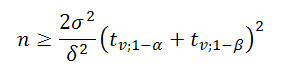
(1) - 4.6
- In our case, the smallest difference to be detected with a significance level of 5 per cent is simply given by the distance between the mean value and the boundary of the 95 per cent-confidence interval.
- 4.7
- Assuming just for the moment, that we would conduct t-tests with equal sample sizes, for the four measures to be tested (number of cooperators and defectors for Settings 1 and 2) it turned out that we would have needed not just 30 runs per Setting of the original model but instead at least 164 runs if we desire a power level of 0.9 (this number reduces to 123 if we are satisfied with a power of 0.8). Since we are not required to base our tests on samples of equal sizes, we are more interested in the required minimum sample size given that Epstein's samples are of size 30. To this end, all we have to do to achieve a rough approximation[5] is to equate the required sample size (in our case 164 runs) with the harmonic mean of Epstein's 30 runs and the number of runs (to be determined) of our replication (Sachs and Hedderich 2009, p. 446).
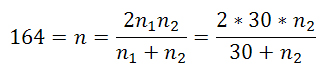
(2) - 4.8
- For the first sample size being 30, it turns out that it's not even possible to construct a test with a power of 80 to 90 per cent. For the second sample size going to infinity, the maximum power to be achieved is close to only 50 per cent, i.e. each time we can't reject a null-hypothesis, there's a 50 per cent-chance, that it is accepted although there is a statistically significant difference between the compared samples (additionally assuming that Epstein's data is indeed distributed normally!). So, while rejected hypotheses still generate significant insights, we have to be very cautious with hypotheses which couldn't be rejected.
- 4.9
- We finally settled with a sample size of 200 runs per combination of true/false-values for the binary parameters, each time using different random seeds for the random number generator for each model corresponding to the parameter settings of Settings 1 and 2. This setup allows for tests with a power of 0.44, so we always have to keep in mind that there's a 56 per cent-chance that a candidate model is not rejected although it produces statistically significantly different data than the original model! Of course, a further increase of the sample size raises statistical power, but the latter is subject to diminishing returns (For a sample size of 1000, the power rises to only 0.48).
- 4.10
- As in the original model we sampled the numbers of cooperators and defectors at t=500 and calculated the mean and the standard deviation which we then tested against the values of the original model by means of Welch's t-test.[6] The results of this endeavor are summarized in the following section.
Results
- 5.1
- Regarding Setting 1, 122 of the 128 candidate models passed the Shapiro-Wilk test for normality at α=0.05. More interestingly, though, in all 122 cases the null hypotheses of equality of means could be rejected for the number of cooperators or the number of defectors at α = 0.05.[7] This high ratio of normally distributed samples gives us at least some confidence, that Epstein's model may indeed have produced normally distributed samples as well. The remaining six cases producing non-normally distributed data can't be evaluated by means of a t-test, but from looking at the mean and standard deviation values we are quite confident nevertheless that none of these resembles the statistical signature of Epstein's model. Therefore, our goal of achieving distributional equivalence was not attained with respect to Setting 1. Please note that the weak power of our tests is not an issue here, because low power amounts to false negatives (type II errors). We, however, have found no negatives at all.
- 5.2
- For Setting 2, only 87 of the 128 candidate models passed the Shapiro-Wilk test at α=0.05. Losing 41 of 128 test cases sounds dramatic, but in fact out of these 41 cases 34 use synchronous updating and are, therefore, ruled out as valid candidates by Epstein's conceptual model. So the actual "loss" in test cases is 7 out of 64 cases using asynchronous updating.[8]
- 5.3
- We were able to reject the null hypothesis of equality of means in 81 of 87 cases, leaving six cases where the results are statistically indistinguishable from the original model. The details of these cases are presented in Table 5. We additionally included another case (in brackets and italic typeset) which seems very close to the values of the original model but didn't pass the test for normality. The table reports the averaged values over 200 runs and additionally the respective standard deviations in parentheses. Furthermore, the results of the t-tests on the equality of means are reported. The asterisk denotes data sets, whose distributions are significantly different from the normal distribution at α=0.05.[9]
Table 5: Details of statistical testing for Setting 2 Parameter No. 1 2 3 4 5 6 7 Original Model (Setting 2) No. Coop. No. Def. 784 (29) 99 (25) Replicated Model (Setting 2) Model No. No. Coop. t-Value No. Def. t-Value (2 T T T T T T F *793,14 (24,83) -1,64 *102,02 (24,43) -0,62) 4 T T T T T F F 793,47 (24,84) -1,70 102,07 (24,35) -0,63 17 T T F T T T T 788,51 (23,70) -0,81 106,92 (23,21) -1,63 66 F T T T T T F 784,83 (28,70) -0,15 91,88 (25,98) 1,45 67 F T T T T F F 787,63 (23,37) -0,65 89,29 (21,24) 2,02 84 F T F T T F F 774,68 (27,38) 1,65 101,68 (23,84) -0,55 99 F T T T T F T 773,54 (23,82) 1,88 102,88 (21,67) -0,81 - 5.4
- Interestingly, the six (plus one) candidate models share a number of features making it even more probable that the respective parameters resemble the choices undertaken in the original model. In Table 5, we have highlighted the corresponding columns of the identified parameters as well as the rows of those models which employ all of these common features. As expected, all cases resembling the results of the original model employ asynchronous updating.
- 5.5
- A little bit more surprising (at least to us) is the result that in all seven candidate solutions agents are born with a random birth age, thereby confirming the description in Epstein's conceptual model which we originally doubted. Assuming random birth age for the agents not only during initialization but throughout the whole simulation run seems counter-intuitive to us, especially if the propagation process is to resemble giving birth[10]. One possible explanation for this assumption is that Epstein, in fact, wanted the individual maximum age of agents to be distributed uniformly between 1 and the maximum age-parameter.[11],[12] We were not able, however, to derive this intention from the description of the conceptual model.
- 5.6
- Another feature employed by all candidate models is that agents die immediately, even if it's not their turn. For the origin of the initial endowment and the shuffling algorithm employed the picture is not quite as clear-cut, but nevertheless a strong majority of the candidate models uses Epstein's shuffling algorithm (as expected) and lets the agents inherit the initial endowment of resources to their offspring.
- 5.7
- Still a little bit more blurry are the results with respect to the first binary parameter remove dead agents immediately. Nevertheless, in the majority of candidate models - four out of six (or four out of seven if we include the candidate model with non-normally distributed data), dead agents are not removed immediately at the time of death but are only removed collectively at the end of each period. This result would be problematic insofar as it contradicts the approach of asynchronous updating to some degree. However, it seems to be too close a call to make a final judgment on the true value of this parameter, especially given the weak power of our hypothesis tests.
- 5.8
- There are exactly three models which share all of the five features identified as probably the ones used by the original model and which differ only by the choice of random number generator and the timing of removal of dead agents. The results of the corresponding statistical tests are highlighted in bold typeset in Table 5. It should be mentioned again that due to the low power of our tests there's a 56 per cent-chance for each of the six (plus one) models that it hasn't been rejected although it should have been. The probability that all six candidate models are false negatives at the same time, however, is rather negligible (about 3 per cent).
- 5.9
- Unfortunately, as a logical consequence of having found not even one plausible parameter combination for Setting 1, we were not able to find a single parameter combination which is capable of reproducing the results of Settings 1 and 2 of the original model at once. We can't rule out the possibility that this is due to an implementation or interpretation error of our own, although we are quite confident that our replication covers the details given in Epstein's conceptual model. An alternative explanation for our inability could be the existence of additional assumptions regarding particularly Setting 1 which were not stated clearly in Epstein (1998) or, to put it differently, that the results of Setting 1 were achieved by a slightly different model than those of Setting 2. Whatever the reason for this finding, in the end we have to admit that our replication was unsuccessful with respect to achieving distributional equivalence.
- 5.10
- The large quantity of data produced in the course of replicating the model led us to the idea to conduct further series of tests regarding the influence of each binary parameter ceteris paribus on the outcomes. Holding six of the seven parameters constant, we compared the two models with the seventh parameter being true and false, this time, however, not with the t-test introduced above. We instead employed the Mann-Whitney test which not only compares the mean values but makes use of the complete samples. The Mann-Whitney test also has the additional advantage that it's a non-parametric statistical test which doesn't require normally distributed samples. Thus, we can evaluate all of the generated samples. The null-hypothesis that both samples are drawn from the same distribution is rejected for p-values below the chosen level of α (again in our case being 0.05).
- 5.11
- This procedure was repeated for all seven parameters and all combinations of the six remaining parameters amounting to 64 tests per Setting and parameter. To illustrate this more vividly, let's consider one specific test on the importance of parameter No. 1, remove dead immediately. Adopting the order of parameters employed in the tables above we have to test 26=64 different combinations of binary parameters having remove dead immediately = true against their counterparts having remove dead immediately = false. Table 6 illustrates this example.
Table 6: An example for a ceteris paribus-analysis of the parameter remove dead immediately Test # Models to compare (Setting 2) p-Value Coop p-Value Def 1-01 #001: TTTTTTT vs. #065: FTTTTTT 0,11 0,00 1-02 #002: TTTTTTF vs. #066: FTTTTTF 0,00 0,00 1-03 #003: TTTTTFT vs. #067: FTTTTFT 0,87 0,00 ... ... ... ... 1-64 #064: TFFFFFF vs. #128: FFFFFFF 0,00 0,00 - 5.12
- All tests are based on the comparison of samples of size 200 generated in the course of conducting the equivalence tests described above. As this short example illustrates, all the candidate models shown differ significantly (p-Values smaller than 0.05) with respect to at least one focal measure, i.e. the compared models produce statistically significantly different outputs. Table 7 summarizes the results of this exercise for all parameters and both Settings.
Table 7: Summary of statistical tests on the influence of parameters Parameter Times H0 is rejected Setting 1 Setting 2 Remove dead agents immediately 64 (100.00%) 64 (100.00%) Die immediately 55 (85.94%) 60 (93.75%) Initial endowment inherited 64 (100.00%) 52 (81.25%) Random birth age 1 (1.56%) 64 (100.00%) Asynchronous updating 64 (100.00%) 64 (100.00%) CERN random 5 (7.81%) 2 (3.13%) Repast list-shuffle 40 (62.50%) 47 (73.44%) - 5.13
- The parameter random birth age confirms what could have been expected a priori. It has no influence at all on the outcomes of Setting 1 (rejecting only 1 of 64 tests) since this Setting assumes no maximum age and therefore the birth age doesn't matter at all. For Setting 2, however, the results vary significantly and produce different outcomes for all 64 cases. This serves as an interesting example of model verification by means of statistical testing.
- 5.14
- A similarly clear picture emerges from the tests on the influence of the updating mechanism. In this instance, the equality of means-null hypothesis is rejected in all cases of Setting 1 and Setting 2, giving additional weight to the importance of choosing the right updating mechanism for the modeling problem at hand. The case is similar with respect to the parameter remove dead immediately. For all possible parameter combinations the samples show a significant difference. The effect is a little bit less pronounced in the case of the parameter die immediately. Still, 55 of 64 parameter combinations show a significant difference for Setting 1 and even 60 of 64 parameter combinations do so for Setting 2. What these three parameters have in common is that they all deal with the timing of events within the model. All these three assumptions concern only the exact point of time during the same global time step when a given procedure should be executed and yet the results vary dramatically. This points out the high importance of explicitly stating the course of events in an agent-based model - for instance by means of a detailed pseudo code[13], flow charts or in the best case a commonly agreed protocol (e.g.Grimm et al. 2006) - in order to be replicable.
- 5.15
- For the assumption about the origin of an offspring's initial endowment the picture is similarly clear as in the above cases. For Setting 2, 52 out of 64 cases show significant differences in the results, depending on the origin of the initial endowment. For Setting 1 the numbers increase to 64 out of 64 cases where the null hypothesis of the samples being drawn from the same distribution has to be rejected.
- 5.16
- As might have been expected, the choice of random library bears no influence on the results.[14] While this might seem common sense, it is nevertheless reassuring that extensive statistical testing confirms this assumption. The case is a little bit different with the choice of a shuffling-algorithm. For both Settings 1 and 2 this choice has a significant influence on the results in the majority of cases (40 of 64 and 47 of 64 cases, respectively), showing that the choice of the shuffling algorithm may be consequential to the outcomes of the model and should therefore be well documented, or probably better, that there should be a common agreement on standard algorithms chosen for such tasks.
Conclusion
- 6.1
- With the benefit of hindsight, the choice of the DPD as a case study probably wasn't a particular wise one given the weaknesses of our statistical tests. Nevertheless, we have learnt a lot from this replication exercise in particular and the systematic method we employed in general.
- 6.2
- With respect to this particular replication exercise, we have to admit that we haven't achieved our goal of distributional equivalence for Settings 1 and 2 at once. However, we were able to replicate the DPD reasonably well regarding Setting 2. This outcome could hint to unstated assumptions regarding the description of the original setting of Setting 1, without which it is not possible to realize a successful replication of the original model. The alternative, of course, is that we have messed up something with regard to Setting 1. But extended and repeated bug tracking raises our confidence that we have implemented Epstein's conceptual model faithfully. Nevertheless, at least on a qualitative level, the replication can be deemed a success with respect to both Settings, for our replication is able to reproduce the basic behaviors identified in the original model, e.g. that cooperation prevails under a wide variety of circumstances.
- 6.3
- By systematic testing of various parameter settings we confirmed that the original model employs asynchronous updating. On the other hand it turned out that it is highly probable, that in the original implementation not only the initial 100 agents start with a random age between one and the given maximum age but also new born agents are initialized with a random age. To us this assumption is rather counter-intuitive for the metaphor of giving birth. We furthermore showed that setting the birth age to one for all new agents, born during a simulation run, produces significantly different results for Setting 2.
- 6.4
- Further analysis of our results revealed the importance of the timing of events in an agent-based model, highlighting the usefulness of explicitly stating the course of events, for instance by means of pseudo code or, better, a commonly agreed protocol like ODD documenting all critical aspects of the model. The use of ontologies (c.f.Polhill and Gotts 2009) also looks promising to alleviate potential problems in communicating model structure. Furthermore, we confirmed the assumption that the choice of random library has no influences on the average results of our replication. The choice of shuffling algorithm, however, does have significant influence in the majority of cases.
- 6.5
- On a more general level, the most important lesson drawn from this exercise is simply that it takes two to tango. This is not a particularly new insight with respect to replication, since many replication efforts only proved successful after the replicators have had extensive communication with the original model authors to clarify ambiguous issues. What is new, however, is that in order to replicate a model quantitatively, the original authors need to not only provide a detailed description of their model, but they also ought to provide enough data to make such a replication effort possible in the first place. Ideally, the full samples should be made available for possible replication attempts.[15] A second-best solution is to provide at least information on the distributional characteristics of the generated data. Obviously, this second solution only makes sense if the model indeed generates normally distributed data. Furthermore, it is already in the modeler's hand to determine the accuracy of future replication attempts by choosing an appropriate sample size.
- 6.6
- We think that our approach of modeling ambiguous assumptions as binary parameters and systematically testing them is a valuable method for the replication of agent-based models which makes extensive use of the verbal description of the model to be replicated as well as the available data. In combination with statistical testing this procedure allows for some kind of reverse engineering when detailed information on the original model is not readily available.
- 6.7
- Nevertheless, we are aware that this method is not free of shortcomings. First, turning ambiguous features into a binary parameter may not always be possible[16]. Second, and even more important, the number of cases to be tested increases exponentially with the binary parameters and therefore our method can only be applied with respect to a selected number of model features, before the evaluation of the generated data turns into an arduous task. Objections might also be raised against our reliance on t-tests but this choice is a concession to the data provided in the original work. In the presence of full samples, more robust tests like the Mann-Whitney test are definitely the first choice, especially when the normal distribution of results can't be guaranteed. For the goal at hand and the process of elimination of candidate solutions, a test on the equality of means is by all means adequate. In our special case study, however, a drop of bitterness remains since we not only had to take distributional assumptions of Epstein's results for granted (which might or might not be the case) but also we had to deal with a comparably low testing power. Despite these considerable objections in the context of this particular model replication, we believe this approach to be a helpful guide in the course of future replication efforts.
Appendix 1: Some Details on Statistical Testing
- A.1
- In this section, we present some additional details on the tests we conducted. Especially, we document the corresponding R-routines in order to make our endeavor more transparent. We provide the raw data sets which we generated in the course of replication for download in the supporting materials.
Sample Size Determination
- A.2
- In order to determine the sample size needed, we made use of existing R-routines. Particularly, with the command
power.t.test
it is possible to arrive at the minimum number needed for conducting two-sample t-tests in the case of equal sample sizes. Given that we conducted two-sided t-tests at a significance level of α=0.05 and we intended to achieve a power of 0.9, all we additionally need to know is the standard deviation of the focal measure and the minimum difference from the mean to be detected at the given significance level. Both measures can be extracted from Epstein (1998) and are summarized for all four focal measures in Table A-1.Table A-1: Detailed values for the standard deviation and delta and minimum sample sizes Focal measure Mean Standard
Deviation95% CI
for the MeanRange of the
Confidence Intervaldelta
(= range/2)Minimum
sample sizeNo. Coop Setting 1 779 15 (773, 784) 11 5.5 158 No. Def Setting 1 121 15 (115, 126) 11 5.5 158 No. Coop Setting 2 784 29 (773, 794) 21 10.5 162 No. Def Setting 2 99 25 (90, 108) 18 9 164 - A.3
- The corresponding R-directive to arrive at the required sample size for the first focal measure is then given by
power.t.test(delta=5.5, sd=15, sig.level=0.05, power=0.9, n=NULL, type="two.sample", alternative="one.sided")
Inserting the delta- and standard deviation-values for the other measures yields the remaining minimum sample sizes. - A.4
- For the further determination of the required minimum sample size for our replication given that Epstein's samples were of size 30, we used the maximum of the minimum sample sizes, i.e. 164. As mentioned in the article, for a rough approximation we can simply equate this minimum sample size with the harmonic mean between Epstein's sample size and our sample size to be determined. For one sample size being 30, however, the harmonic mean converges to 60 in the limit, thereby showing that a test with a power of 0.9 is simply not feasible. For our sample size going to infinity, the test would have yielded a power of about 0.5. This can easily be calculated by inserting the harmonic mean into the
power.t.test
routine leaving the power-parameter undetermined.power.t.test(delta=9, sd=25, sig.level=0.05, power=NULL, n=60, type="two.sample", alternative="one.sided")
This time we have used as parameters the values of the run requiring the largest minimum sample size. - A.5
- So, we had to accept a lower power and settled for a sample size of 200, which is large enough to surely level out influences of the random seeds of the particular runs. Increasing the sample size even further brings disproportionally few additional benefits in terms of power. The harmonic mean between the two sample sizes (30 and 200, respectively) is approximately 52. Again with the help of
power.t.test
we can calculate the power of the resulting test.power.t.test(delta=9, sd=25, sig.level=0.05, power=NULL, n=52, type="two.sample", alternative="one.sided")
The power of this test is then 0.44.Testing for Normality
- A.6
- Testing for normality is a straight forward exercise in R. We chose to use the Shapiro-Wilk test (we additionally tested our samples with the Anderson-Darling test but the results were to a large degree similar). The corresponding routine in R is
shapiro.test(samplename)
The null-hypothesis that the sample is indeed distributed normally is rejected for p-values below the chosen significance level (in our case 0.05).Welch's t-Test
- A.7
- In the case of the Welch test we passed on using R and instead simply calculated the test statistics using spreadsheets. The formula for this test is given by
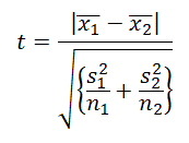
(A.1) where the numerator represents the difference between the samples' means and s2 and n are the sample variance and sample size, respectively. The degrees of freedom are given by v = n2 - 1 for n2 < n1 or, more accurately, with the help of the Welch-Satterthwaite equation:
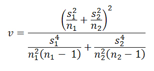
(A.2) The null-hypothesis of equality of means is rejected if the test statistic exceeds the respective critical value of the Student-distribution.
Mann-Whitney Test
- A.8
- The Mann-Whitney test can be considered as an analogue to the t-test in the case that the samples are not necessarily distributed normally and is often used for similar purposes. The null-hypothesis states that the two samples to be compared are drawn from the same distribution. This hypothesis is rejected for p-values below the desired significance level (in our case again being 0.05). The corresponding R command is given by
wilcox.test
which calculates an approximate test statistic. For an exact calculation we referred to a modification of this procedure available through the package exactRankTests.wilcox.exact(samplename1, samplename2, alternative="two.sided")
- A.9
- In the supporting materials we also make available for download our datasets which can be further analyzed with statistical software packages.
Appendix 2: Results
-
Table A-2: Results of the replication of Run 1 Parameter No. 1 2 3 4 5 6 7 Original Model (Run 1) No. Coop. No. Def. 779 (15) 121 (15) Replicated Model (Run 1) Setting No. No. Coop. t-Value No. Def. t-Value 1 T T T T T T T 753,12 (16,99) 8,66 146,83 (17,00) -8,63 2 T T T T T T F 749,02 (16,26) 10,09 150,85 (16,24) -10,05 3 T T T T T F T 755,49 (16,91) 7,87 144,46 (16,90) -7,85 4 T T T T T F F 746,44 (17,77) 10,81 153,46 (17,75) -10,78 5 T T T T F T T 718,59 (26,28) 18,25 181,24 (26,22) -18,22 6 T T T T F T F 711,78 (26,78) 20,19 188,08 (26,77) -20,15 7 T T T T F F T 720,58 (27,22) 17,45 179,31 (27,18) -17,43 8 T T T T F F F 713,08 (26,43) 19,88 186,79 (26,36) -19,86 9 T T T F T T T 752,73 (15,62) 8,90 147,23 (15,60) -8,88 10 T T T F T T F 747,28 (16,08) 10,70 152,63 (16,07) -10,67 11 T T T F T F T 756,34 (15,81) 7,66 143,59 (15,79) -7,64 12 T T T F T F F 747,17 (15,89) 10,75 152,72 (15,88) -10,72 13 T T T F F T T 715,40 (26,23) 19,23 184,46 (26,22) -19,19 14 T T T F F T F 710,99 (28,13) 20,09 188,89 (28,09) -20,07 15 T T T F F F T 717,63 (26,12) 18,58 182,26 (26,09) -18,55 16 T T T F F F F 714,39 (26,21) 19,54 185,47 (26,16) -19,51 17 T T F T T T T 731,77 (18,07) 15,63 168,15 (18,07) -15,60 18 T T F T T T F 724,83 (16,45) 18,21 175,06 (16,39) -18,18 19 T T F T T F T 727,48 (17,52) 17,14 172,42 (17,49) -17,11 20 T T F T T F F 722,23 (19,14) 18,58 177,59 (19,11) -18,53 21 T T F T F T T 680,02 (30,46) 28,41 219,72 (30,36) -28,37 22 T T F T F T F *670,56 (57,83) 22,03 *224,75 (36,22) -27,67 23 T T F T F F T 679,95 (31,25) 28,15 219,79 (31,13) -28,12 24 T T F T F F F 671,41 (30,99) 30,67 228,32 (30,81) -30,67 25 T T F F T T T 729,11 (16,19) 16,81 170,81 (16,21) -16,78 26 T T F F T T F 723,81 (16,77) 18,49 176,06 (16,72) -18,46 27 T T F F T F T 732,96 (19,28) 15,05 166,96 (19,26) -15,03 28 T T F F T F F 724,07 (19,04) 17,93 175,61 (19,00) -17,90 29 T T F F F T T 680,97 (31,28) 27,85 218,79 (31,17) -27,81 30 T T F F F T F 669,20 (32,44) 30,74 230,49 (32,32) -30,69 31 T T F F F F T 678,21 (29,15) 29,40 221,58 (29,07) -29,37 32 T T F F F F F 671,82 (34,20) 29,34 227,89 (34,05) -29,31 33 T F T T T T T 748,03 (14,51) 10,59 151,85 (14,44) -10,56 34 T F T T T T F 741,65 (15,36) 12,68 158,16 (15,37) -12,61 35 T F T T T F T 748,15 (15,80) 10,43 151,73 (15,75) -10,39 36 T F T T T F F 743,00 (16,42) 12,10 156,67 (16,32) -12,00 37 T F T T F T T 690,15 (25,82) 27,00 209,68 (25,75) -26,96 38 T F T T F T F 687,14 (24,25) 28,43 212,61 (24,20) -28,37 39 T F T T F F T 689,17 (25,98) 27,24 210,59 (25,93) -27,18 40 T F T T F F F 683,91 (25,26) 29,08 215,87 (25,10) -29,07 41 T F T F T T T 747,93 (14,33) 10,64 151,93 (14,34) -10,59 42 T F T F T T F 740,43 (15,89) 13,03 159,32 (15,82) -12,95 43 T F T F T F T 747,72 (14,46) 10,70 152,15 (14,44) -10,66 44 T F T F T F F 741,54 (14,95) 12,76 158,19 (14,95) -12,67 45 T F T F F T T 690,72 (23,62) 27,52 209,06 (23,58) -27,46 46 T F T F F T F 683,53 (26,59) 28,74 216,27 (26,52) -28,70 47 T F T F F F T 688,12 (28,75) 26,64 211,72 (28,72) -26,61 48 T F T F F F F 683,80 (26,88) 28,56 216,01 (26,86) -28,51 49 T F F T T T T 731,71 (15,84) 15,98 168,08 (15,84) -15,91 50 T F F T T T F 727,20 (16,05) 17,47 172,45 (15,97) -17,37 51 T F F T T F T 731,03 (15,44) 16,27 168,84 (15,45) -16,22 52 T F F T T F F 722,66 (16,25) 18,97 176,93 (16,17) -18,84 53 T F F T F T T 656,04 (30,58) 35,24 243,68 (30,53) -35,18 54 T F F T F T F 649,69 (31,18) 36,78 249,89 (30,96) -36,76 55 T F F T F F T 654,70 (31,21) 35,34 244,94 (31,15) -35,27 56 T F F T F F F 653,87 (29,69) 36,26 245,77 (29,58) -36,20 57 T F F F T T T 728,75 (14,32) 17,21 171,06 (14,32) -17,15 58 T F F F T T F 727,04 (16,72) 17,42 172,63 (16,65) -17,32 59 T F F F T F T 730,23 (16,03) 16,46 169,61 (16,01) -16,40 60 T F F F T F F 724,31 (15,63) 18,52 175,40 (15,61) -18,42 61 T F F F F T T 659,57 (31,91) 33,66 240,09 (31,68) -33,66 62 T F F F F T F 649,58 (30,75) 37,01 250,11 (30,56) -37,01 63 T F F F F F T 654,64 (29,46) 36,14 244,98 (29,30) -36,10 64 T F F F F F F 653,94 (29,83) 36,18 245,77 (29,70) -36,15 65 F T T T T T T 744,63 (18,51) 11,32 154,38 (18,27) -11,02 66 F T T T T T F 734,52 (19,26) 14,54 163,93 (18,87) -14,09 67 F T T T T F T 745,31 (18,24) 11,13 153,62 (18,04) -10,80 68 F T T T T F F 737,63 (19,65) 13,47 160,80 (19,31) -13,01 69 F T T T F T T 810,66 (12,44) -11,01 89,28 (12,39) 11,03 70 F T T T F T F 811,11 (12,49) -11,16 88,86 (12,47) 11,17 71 F T T T F F T 811,82 (12,24) -11,43 88,13 (12,26) 11,44 72 F T T T F F F 809,10 (12,20) -10,48 90,85 (12,21) 10,50 73 F T T F T T T 743,83 (16,60) 11,81 155,17 (16,39) -11,49 74 F T T F T T F 735,78 (17,89) 14,33 162,56 (17,58) -13,82 75 F T T F T F T 747,63 (16,82) 10,51 151,41 (16,65) -10,20 76 F T T F T F F 735,90 (18,91) 14,14 162,55 (18,71) -13,66 77 F T T F F T T 810,17 (12,67) -10,82 89,77 (12,64) 10,84 78 F T T F F T F 809,43 (12,20) -10,60 90,47 (12,21) 10,63 79 F T T F F F T 812,14 (13,02) -11,47 87,80 (13,01) 11,49 80 F T T F F F F 809,85 (13,10) -10,67 90,04 (13,05) 10,71 81 F T F T T T T 722,62 (17,82) 18,70 176,05 (17,55) -18,31 82 F T F T T T F 713,66 (20,82) 21,01 184,26 (20,28) -20,46 83 F T F T T F T *722,71 (17,75) 18,68 *175,81 (17,48) -18,24 84 F T F T T F F 711,71 (18,11) 22,26 186,08 (17,48) -21,66 85 F T F T F T T 799,76 (14,25) -7,11 100,16 (14,22) 7,14 86 F T F T F T F 802,08 (14,58) -7,89 97,84 (14,56) 7,92 87 F T F T F F T 800,56 (13,07) -7,46 99,28 (13,06) 7,51 88 F T F T F F F 798,63 (13,23) -6,78 101,26 (13,17) 6,83 89 F T F F T T T 723,60 (18,08) 18,33 174,83 (17,69) -17,88 90 F T F F T T F 714,31 (19,02) 21,20 183,65 (18,63) -20,61 91 F T F F T F T 724,00 (17,00) 18,39 174,82 (16,82) -18,03 92 F T F F T F F 712,00 (20,02) 21,73 185,91 (19,63) -21,14 93 F T F F F T T 801,08 (14,70) -7,54 98,85 (14,67) 7,56 94 F T F F F T F 801,65 (13,30) -7,82 98,29 (13,29) 7,85 95 F T F F F F T 802,11 (14,15) -7,96 97,72 (14,11) 7,99 96 F T F F F F F 800,63 (14,62) -7,39 99,27 (14,59) 7,43 97 F F T T T T T 724,82 (16,96) 18,12 173,86 (16,83) -17,70 98 F F T T T T F 711,63 (18,91) 22,11 186,08 (18,49) -21,44 99 F F T T T F T 724,46 (16,16) 18,38 174,02 (15,78) -17,93 100 F F T T T F F 714,74 (19,03) 21,06 183,16 (18,49) -20,48 101 F F T T F T T *799,16 (12,68) -7,00 *100,78 (12,63) 7,02 102 F F T T F T F 797,50 (12,44) -6,43 102,42 (12,45) 6,46 103 F F T T F F T 797,58 (13,35) -6,41 102,36 (13,32) 6,44 104 F F T T F F F 797,35 (12,98) -6,35 102,60 (12,97) 6,37 105 F F T F T T T 724,44 (17,51) 18,15 174,02 (17,15) -17,70 106 F F T F T T F 713,82 (20,45) 21,05 183,96 (19,95) -20,44 107 F F T F T F T 721,99 (17,84) 18,91 176,40 (17,73) -18,39 108 F F T F T F F 712,73 (18,93) 21,74 184,98 (18,28) -21,13 109 F F T F F T T 795,79 (11,99) -5,86 104,13 (11,97) 5,89 110 F F T F F T F *797,76 (13,14) -6,49 *102,14 (13,11) 6,52 111 F F T F F F T 795,60 (11,89) -5,79 104,26 (11,86) 5,85 112 F F T F F F F 797,47 (12,50) -6,42 102,43 (12,44) 6,46 113 F F F T T T T 704,75 (19,41) 24,24 193,25 (19,04) -23,67 114 F F F T T T F 692,90 (19,68) 28,03 203,98 (19,13) -27,17 115 F F F T T F T 703,41 (17,06) 25,26 194,41 (16,70) -24,61 116 F F F T T F F 692,13 (19,83) 28,23 204,95 (19,27) -27,45 117 F F F T F T T 786,50 (13,48) -2,58 113,39 (13,46) 2,62 118 F F F T F T F 786,13 (12,65) -2,47 113,78 (12,62) 2,51 119 F F F T F F T 786,75 (13,63) -2,67 113,17 (13,61) 2,70 120 F F F T F F F 788,28 (13,63) -3,19 111,67 (13,59) 3,21 121 F F F F T T T 703,77 (18,76) 24,72 194,47 (18,45) -24,22 122 F F F F T T F *690,83 (19,12) 28,87 206,18 (18,69) -28,01 123 F F F F T F T 704,28 (17,00) 24,98 193,92 (16,70) -24,45 124 F F F F T F F 694,01 (19,83) 27,63 202,95 (19,22) -26,80 125 F F F F F T T 788,02 (14,18) -3,09 111,85 (14,15) 3,14 126 F F F F F T F *787,95 (12,96) -3,10 *111,90 (12,95) 3,15 127 F F F F F F T 787,09 (12,52) -2,81 112,78 (12,52) 2,86 128 F F F F F F F 787,98 (12,23) -3,13 111,91 (12,21) 3,17 Table A-3: Results of the replication of Run 2 Parameter No. 1 2 3 4 5 6 7 Original Model (Run 2) No. Coop. No. Def. 784 (29) 99 (25) Replicated Model (Run 2) Setting No. No. Coop. t-Value No. Def. t-Value 1 T T T T T T T 802,86 (25,69) -3,37 93,08 (25,18) -1,21 2 T T T T T T F *793,14 (24,83) -1,64 *102,02 (24,43) -0,62 3 T T T T T F T 803,77 (26,10) -3,52 91,99 (25,80) 1,43 4 T T T T T F F 793,47 (24,84) -1,70 102,07 (24,35) -0,63 5 T T T T F T T 455,71 (21,46) 59,60 412,03 (18,39) -65,96 6 T T T T F T F *446,99 (38,92) 56,48 *414,85 (34,87) -60,88 7 T T T T F F T 457,36 (22,70) 59,04 411,05 (18,79) -65,64 8 T T T T F F F 449,90 (20,40) 60,80 415,94 (17,22) -67,09 9 T T T F T T T *733,43 (23,21) 9,12 *165,32 (22,81) -13,70 10 T T T F T T F 721,27 (25,49) 11,22 176,74 (25,13) -15,87 11 T T T F T F T 733,94 (24,22) 8,46 161,69 (24,01) -12,87 12 T T T F T F F 724,61 (24,42) 10,67 173,17 (23,73) -15,25 13 T T T F F T T 471,14 (24,16) 56,24 413,70 (21,40) -65,44 14 T T T F F T F 456,98 (21,99) 59,26 425,63 (18,83) -68,70 15 T T T F F F T 471,27 (20,96) 56,88 414,06 (18,85) -66,26 16 T T T F F F F 457,94 (22,10) 59,06 424,92 (18,96) -68,51 17 T T F T T T T 788,51 (23,70) -0,81 106,92 (23,21) -1,63 18 T T F T T T F 774,02 (25,95) -1,78 121,03 (25,41) -4,49 19 T T F T T F T 785,55 (24,39) -0,28 *110,29 (24,00) -2,32 20 T T F T T F F 772,03 (25,39) 2,14 123,13 (24,95) -4,93 21 T T F T F T T 417,89 (24,69) 65,67 444,42 (20,49) -72,13 22 T T F T F T F 408,23 (22,86) 67,88 451,52 (17,58) -74,52 23 T T F T F F T 417,25 (24,74) 65,77 446,73 (20,56) -72,59 24 T T F T F F F 410,48 (24,10) 67,16 450,12 (18,93) -73,82 25 T T F F T T T 708,54 (23,24) 13,61 189,88 (22,94) -18,76 26 T T F F T T F 694,39 (25,79) 16,00 202,99 (25,32) -21,21 27 T T F F T F T 708,99 (25,69) 13,40 189,20 (25,35) -18,39 28 T T F F T F F 692,88 (23,27) 16,43 204,45 (22,62) -21,80 29 T T F F F T T 426,67 (24,16) 64,23 454,19 (21,08) -73,97 30 T T F F F T F 415,87 (22,34) 66,63 462,37 (19,56) -76,19 31 T T F F F F T 427,25 (23,56) 64,27 453,64 (20,14) -74,14 32 T T F F F F F 413,96 (23,12) 66,78 463,51 (19,60) -76,41 33 T F T T T T T *846,14 (17,27) -11,44 *49,81 (16,91) 10,43 34 T F T T T T F 826,82 (22,89) -7,73 *68,63 (22,02) 6,30 35 T F T T T F T 845,87 (15,98) -11,43 49,89 (15,54) 10,46 36 T F T T T F F 828,48 (20,23) -8,11 66,91 (19,47) 6,73 37 T F T T F T T 457,76 (20,73) 59,38 410,05 (17,18) -65,86 38 T F T T F T F 458,53 (21,87) 59,01 408,17 (17,46) -65,39 39 T F T T F F T 461,38 (21,98) 58,47 407,29 (18,62) -64,90 40 T F T T F F F 458,81 (22,75) 58,77 407,57 (19,00) -64,85 41 T F T F T T T 779,19 (21,14) 0,87 119,32 (20,75) -4,24 42 T F T F T T F 754,17 (21,20) 5,42 143,40 (20,55) -9,27 43 T F T F T F T 780,65 (20,96) 0,61 117,97 (20,49) -3,96 44 T F T F T F F 750,51 (23,44) 6,04 146,81 (22,73) -9,88 45 T F T F F T T 468,62 (20,81) 57,39 415,78 (17,78) -66,91 46 T F T F F T F 464,32 (22,64) 57,79 *418,33 (19,83) -66,88 47 T F T F F F T 468,06 (21,98) 57,26 415,90 (19,54) -66,45 48 T F T F F F F 461,63 (23,43) 58,11 420,33 (20,09) -67,22 49 T F F T T T T 837,81 (20,14) -9,81 58,06 (19,70) 8,58 50 T F F T T T F *817,86 (22,37) -6,13 *77,02 (21,24) 4,57 51 T F F T T F T 840,17 (18,04) -10,31 55,60 (17,71) 9,17 52 T F F T T F F 816,81 (23,61) -5,91 77,76 (22,81) 4,39 53 T F F T F T T 423,02 (22,26) 65,35 440,32 (18,00) -72,03 54 T F F T F T F 420,37 (23,60) 65,50 440,34 (18,88) -71,78 55 T F F T F F T 426,83 (20,21) 65,13 437,92 (16,94) -71,82 56 T F F T F F F 419,77 (22,61) 65,86 440,82 (18,45) -72,00 57 T F F F T T T 767,49 (21,18) 3,00 130,99 (20,82) -6,67 58 T F F F T T F 735,33 (22,44) 8,81 161,23 (21,65) -12,93 59 T F F F T F T 768,79 (23,79) 2,74 129,60 (23,45) -6,30 60 T F F F T F F 737,65 (22,96) 8,37 159,29 (22,11) -12,50 61 T F F F F T T 429,29 (22,56) 64,15 451,18 (19,43) -73,89 62 T F F F F T F 426,07 (21,41) 65,00 453,31 (17,28) -74,99 63 T F F F F F T 432,13 (21,19) 63,95 447,98 (17,36) -73,83 64 T F F F F F F 426,63 (23,18) 64,48 452,29 (19,21) -74,18 65 F T T T T T T *806,32 (23,07) -4,03 *72,64 (21,27) 5,49 66 F T T T T T F 784,83 (28,70) -0,15 91,88 (25,98) 1,45 67 F T T T T F T 803,97 (21,45) -3,63 74,85 (20,14) 5,05 68 F T T T T F F 787,63 (23,37) -0,65 89,29 (21,24) 2,02 69 F T T T F T T *866,07 (11,91) -15,31 *15,67 (10,38) 18,03 70 F T T T F T F *867,87 (12,04) -15,64 *14,22 (11,05) 18,31 71 F T T T F F T *866,95 (11,88) -15,47 *15,29 (10,79) 18,09 72 F T T T F F F *868,54 (10,91) -15,80 *13,53 (9,87) 18,51 73 F T T F T T T 728,38 (26,43) 9,91 160,70 (24,21) -12,66 74 F T T F T T F 696,63 (27,11) 15,52 188,34 (24,50) -18,30 75 F T T F T F T 726,84 (25,46) 10,22 162,02 (23,27) -12,99 76 F T T F T F F 696,78 (27,82) 15,42 187,91 (24,87) -18,18 77 F T T F F T T *871,17 (13,20) -16,21 *27,79 (12,97) 15,30 78 F T T F F T F *871,06 (12,94) -16,20 *27,81 (12,70) 15,30 79 F T T F F F T *871,90 (12,57) -16,37 *27,08 (12,41) 15,47 80 F T T F F F F *871,50 (12,74) -16,29 *27,49 (12,60) 15,38 81 F T F T T T T 792,92 (23,70) -1,61 84,80 (21,41) 2,95 82 F T F T T T F 772,13 (25,96) 2,12 103,68 (23,67) -0,96 83 F T F T T F T 793,79 (26,33) -1,74 84,16 (23,61) 3,05 84 F T F T T F F 774,68 (27,38) 1,65 101,68 (23,84) -0,55 85 F T F T F T T *865,59 (12,49) -15,20 *16,87 (11,41) 17,72 86 F T F T F T F *868,72 (10,89) -15,83 *13,97 (9,70) 18,42 87 F T F T F F T *866,72 (12,54) -15,41 *15,53 (11,23) 18,02 88 F T F T F F F *867,66 (11,17) -15,63 *14,54 (9,87) 18,29 89 F T F F T T T 705,73 (26,39) 13,94 181,52 (24,04) -16,94 90 F T F F T T F 672,58 (26,66) 19,83 209,50 (23,53) -22,75 91 F T F F T F T 706,15 (25,17) 13,94 181,02 (22,88) -16,94 92 F T F F T F F 676,53 (27,89) 19,02 206,28 (25,52) -21,86 93 F T F F F T T *867,41 (14,18) -15,48 *31,34 (13,87) 14,49 94 F T F F F T F *869,43 (13,48) -15,88 *29,49 (13,31) 14,92 95 F T F F F F T 867,98 (13,39) -15,61 30,67 (13,20) 14,67 96 F T F F F F F *869,27 (12,22) -15,89 *29,40 (12,08) 14,99 97 F F T T T T T 770,01 (26,63) 2,49 105,84 (24,52) -1,40 98 F F T T T T F 749,25 (30,01) 6,09 124,66 (26,89) -5,19 99 F F T T T F T 773,54 (23,82) 1,88 102,88 (21,67) -0,81 100 F F T T T F F 751,79 (26,48) 5,74 122,29 (23,24) -4,80 101 F F T T F T T *862,75 (12,54) -14,67 *19,54 (11,67) 17,13 102 F F T T F T F *862,43 (13,78) -14,57 *19,60 (12,47) 17,08 103 F F T T F F T *863,02 (13,87) -14,67 *19,53 (12,84) 17,08 104 F F T T F F F *862,77 (13,11) -14,65 *19,98 (12,01) 17,02 105 F F T F T T T 685,52 (29,06) 17,34 199,52 (25,91) -20,44 106 F F T F T T F 652,66 (26,45) 23,39 226,65 (22,78) -26,37 107 F F T F T F T 689,32 (27,00) 16,82 195,33 (24,33) -19,75 108 F F T F T F F 647,72 (28,49) 24,06 231,04 (24,96) -26,98 109 F F T F F T T *864,77 (14,52) -14,98 *33,84 (14,13) 13,95 110 F F T F F T F *866,90 (14,84) -15,36 *31,83 (14,51) 14,36 111 F F T F F F T *864,13 (15,20) -14,83 *34,45 (14,87) 13,78 112 F F T F F F F *865,74 (13,81) -15,18 *32,82 (13,53) 14,19 113 F F F T T T T 768,77 (30,51) 2,66 107,57 (26,65) -1,74 114 F F F T T T F 737,75 (31,89) 8,04 135,12 (28,38) -7,24 115 F F F T T F T 762,63 (28,29) 3,78 112,84 (25,26) -2,82 116 F F F T T F F 734,33 (29,68) 8,72 138,50 (26,39) -8,01 117 F F F T F T T *860,60 (13,34) -14,24 *21,85 (12,44) 16,60 118 F F F T F T F *863,25 (14,85) -14,68 *18,86 (13,69) 17,18 119 F F F T F F T *863,81 (12,49) -14,87 *18,40 (12,12) 17,36 120 F F F T F F F *860,76 (13,28) -14,27 *20,82 (12,49) 16,82 121 F F F F T T T 666,29 (26,82) 20,93 216,72 (24,50) -24,11 122 F F F F T T F *627,59 (52,04) 24,26 *244,73 (29,19) -29,09 123 F F F F T F T 668,10 (28,18) 20,49 214,67 (25,16) -23,61 124 F F F F T F F 630,12 (27,90) 27,23 246,74 (24,21) -30,31 125 F F F F F T T *862,35 (14,82) -14,52 *36,20 (14,46) 13,43 126 F F F F F T F *860,50 (15,27) -14,16 *37,95 (15,07) 13,02 127 F F F F F F T 863,41 (14,11) -14,74 35,10 (13,72) 13,69 128 F F F F F F F *861,78 (13,22) -14,47 *36,64 (13,00) 13,39
Acknowledgements
- Wolfgang Radax's contribution to this paper is funded by research grant #P19973 of the Austrian Science Fund FWF. An earlier version of this paper was presented at the ESSA 2009 conference. We would like to thank the participants for many insightful comments. We give special thanks to ESSA and Volterra Consulting for calling into existence the Volterra Replication Prize. This occasion was the original motivation for the present article. Bernhard Böhm and Klaus Prettner provided valuable advice on statistical testing. We are also indebted to two anonymous referees whose penetrating comments and suggestions helped us tremendously in shaping our argument. Furthermore, we explicitly express our gratitude to Professor Epstein for providing his source code.
Notes
-
1 We ran a reimplementation of the model provided with the accompanying CD-ROM of Epstein (2007) a few times. The CD-ROM only contained an executable version of the model, source code was not provided.
2 Professor Epstein did not receive two e-mails sent by us in February and March, 2009, respectively. Thanks to the editor's intervention he eventually sent us his original source code, written in C++, on March 18th, 2010. The provided code is the one that was used for his 1998 article. We wish to express gratitude for sharing his research code with us.
3 The original model describes a per-se deterministic process, which of course leads to the same result when simulated using the same parameters and the same random seed. If we believe, that the simulated process is precise, then the overall effect of varying the random element should be considerably smaller than the effect of varying simulation parameters. A precise process should lead to similar results when only the random element is varied, so the results of different runs should cluster around an average value (i.e. ideally they should be normally distributed). For the concept of precision in model building see North and Macal (2007), p. 18.
4 Details about the determination of sample size and the statistical tests used throughout the paper can be found in the Appendix.
5 This approximation is rather rough because we hold the t-values constant, although the degrees of freedoms would have to be determined endogenously. But since the t-values are rather close to 2 in any case, the resulting imprecision can be neglected for achieving a first approximation.
6 Using two t-tests for the numbers of cooperators and defectors, respectively, implicitly implies statistical independence between these two measures. Indeed, this assumption is not unusual in statistical testing of replications (see, for instance,Wilensky and Rand 2007). For the more plausible (and probably methodologically sounder) assumption of statistical dependence between the numbers of cooperators and defectors, multivariate two-sample tests like Hotelling's T2 would be in order. Since we only have mean values and variances, but not the full samples of the original model at our disposal, such tests can't be applied for the problem at hand. Using univariate tests instead introduces bias into our testing procedure. Exact statements about the size and direction of such a bias, however, can't be made without recourse to mathematical statistics.
7 Detailed results of all 128 candidate models for Setting 1 are provided in the appendix (Table A-2).
8 A related interesting issue worth pursuing in the future is whether this correlation between synchronous updating and non-normally distributed data is only an artifact of this particular model or an indication for a more general finding.
9 Again, detailed results of all 128 candidate models for Setting 2 provided in the appendix (Table A-3).
10 In his Ascape reimplementation, Epstein (2007) no longer calls the propagation process, giving birth, but calls it fissioning instead (Model Settings Screen, Rules Section).
11 We would like to thank Ken Kahn for this suggestion.
12 In an e-mail received in March 2010, Professor Epstein explained the rationale of him using random birth age for his agents stating that "This was obviously a coding convenience adopted to ensure a uniform age distribution bounded above by Max_Age."
13 While writing this paper we realized that pseudo code is as prone to ambiguities as plain verbal description, if it is not used with great care for details. However, pseudo code forces the modeler to state the order of events in a strictly sequential way. We received suggestions that plain verbal description of the model can do the trick as well if it is complete, but contrary to the other methods proposed it does not force you to be as explicit, thereby usually not arriving at the same level of clarity.
145 out of 64 cases, however, is still a very high number of rejections for Setting 1 given that there should be absolutely no difference on average. This is surely an issue to be further investigated.
15 In the best case, the original model author provides access to the source code. The replicator can then generate her own samples for analysis.
16 As one referee has pointed out correctly, this method is not restricted to binary options. Any parameter having a discrete number of possible values can be included. The number of tests to be conducted rises correspondingly.
References
-
AXTELL, R, Axelrod, R, Epstein, J M and Cohen, M D (1996) Aligning Simulation Models: A Case Study and Results. Computational and Mathematical Organization Theory 1: 123-141. [doi:10.1007/BF01299065]
BIGBEE, T, Cioffi-Revilla, C and Luke, S (2007) Replication of Sugarscape using MASON. In Terano, T, Kita, H, Deguchi,H and Kijima, K (eds.) Agent-Based Approaches in Economic and Social Complex Systems IV: 183-190. Japan: Springer. [doi:10.1007/978-4-431-71307-4_20]
EDMONDS, B and Hales, D (2003) Replication, Replication and Replication: Some Hard Lessons from Model Alignment. Journal of Artificial Societies and Social Simulation 6(4)11 < https://www.jasss.org/6/4/11.html >.
EDMONDS, B and Hales, D (2005) Computational Simulation as Theoretical Experiment. Journal of Mathematical Sociology 29: 1-24. [doi:10.1080/00222500590921283]
EPSTEIN, J M (1998) Zones of Cooperation in Demographic Prisoner's Dilemma. Complexity 4(2): 36-48. [doi:10.1002/(SICI)1099-0526(199811/12)4:2<36::AID-CPLX9>3.0.CO;2-Z]
EPSTEIN, J M (2007) Generative Social Science: Studies in Agent-Based Computational Modeling (Princeton Studies of Complexity). Princeton, NJ: Princeton University Press.
GALAN, J M and Izquierdo, L R (2005) Appearances Can Be Deceiving: Lessons Learned Re-Implementing Axelrod's 'Evolutionary Approach to Norms'. Journal of Artificial Societies and Social Simulation 8(3)2 < https://www.jasss.org/8/3/2.html >.
GALAN J M, Izquierdo L R, Izquierdo S S, Santos J I, del Olmo, R, Lopez-Paredes, A and Edmonds B (2009) Errors and Artefacts in Agent-Based Modelling. Journal of Artificial Societies and Social Simulation 12(1)1 < https://www.jasss.org/12/1/1.html >.
GRIMM, V, Berger, U, Bastiansen, F, Eliassen, S, Ginot, V, Giske, J, Goss-Custard, J, Grand, T, Heinz, S K, Huse, G, Huth, A, Jepsen, J U, Jorgensen, C, Mooij, W M, Müller, B, Pe'er, G, Piou, C, Railsback, S F, Robbins, A M, Robbins, M M, Rossmanith, E, Rüger, N, Strand, E, Souissi, S, Stillman, R A, Vabo, R, Visser, U and DeAngelis, D L (2006) A standard protocol for describing individual-based and agent-based models. Ecological Modelling 198: 115-126. [doi:10.1016/j.ecolmodel.2006.04.023]
HALES, D, Rouchier, J and Edmonds, B (2003) Model-to-Model Analysis. Journal of Artificial Societies and Social Simulation 6(4)5 < https://www.jasss.org/6/4/5.html >.
HUBERMAN, B A and Glance, N S (1993) Evolutionary games and computer simulations. Proceedings of the National Academy of Sciences USA 90: 7716-7718. [doi:10.1073/pnas.90.16.7716]
IZQUIERDO, L R, Izquierdo, S S, Galan, J M and Santos, J I (2009) Techniques to Understand Computer Simulations: Markov Chain Analysis. Journal of Artificial Societies and Social Simulation 12(1)6 < https://www.jasss.org/12/1/6.html >.
NORTH, M J and Macal, C M (2007) Managing business complexity: discovering strategic solutions with agent-based modeling and simulation. New York: Oxford University Press. [doi:10.1093/acprof:oso/9780195172119.001.0001]
NORTH, M J, Collier, N T and Vos J R (2006) Experiences Creating Three Implementations of the Repast Agent Modeling Toolkit. ACM Transactions on Modeling and Computer Simulation, Vol. 16(1): 1-25. [doi:10.1145/1122012.1122013]
Nowak, M A and May, R M (1992) Evolutionary games and spatial chaos. Nature 359: 826-829. [doi:10.1038/359826a0]
POLHILL, J G and Gotts, N M (2009) Ontologies for transparent integrated human-natural system modeling. Landscape Ecology 24: 1255-67. [doi:10.1007/s10980-009-9381-5]
ROUCHIER, J (2003) Re-implementation of a multi-agent model aimed at sustaining experimental economic research: The case of simulations with emerging speculation. Journal of Artificial Societies and Social Simulation 6(4)7 < https://www.jasss.org/6/4/7.html >.
ROUCHIER, J, Cioffi-Revilla, C, Polhill J G and Takadama K (2008) Progress in Model-To-Model Analysis. Journal of Artificial Societies and Social Simulation 11(2)8 < https://www.jasss.org/11/2/8.html >.
SACHS, L and Hedderich, J (2009) Angewandte Statistik: Methodensammlung mit R, 13th revised and extended Edition. Berlin: Springer.
WILENSKY, U and Rand, W (2007) Making Models Match: Replicating an Agent-Based Model. Journal of Artificial Societies and Social Simulation 10(4)2 < https://www.jasss.org/10/4/2.html >.
WILL, O (2009) Resolving a Replication That Failed: News on the Macy & Sato Model. Journal of Artificial Societies and Social Simulation 12(4)11 < https://www.jasss.org/12/4/11.html >.
WILL, O and Hegselmann, R (2008) A Replication That Failed - on the Computational Model in 'Michael W. Macy and Yoshimichi Sato: Trust, Cooperation and Market Formation in the U.S. and Japan. Proceedings of the National Academy of Sciences, May 2002'. Journal of Artificial Societies and Social Simulation 11(3)3 < https://www.jasss.org/11/3/3.html >.