
 Abstract
- We have studied how leaders emerge in a group as a consequence of interactions among its members. We propose that leaders can emerge as a consequence of a self-organized process based on local rules of dyadic interactions among individuals. Flocks are an example of self-organized behaviour in a group and properties similar to those observed in flocks might also explain some of the dynamics and organization of human groups. We developed an agent-based model that generated flocks in a virtual world and implemented it in a multi-agent simulation computer program that computed indices at each time step of the simulation to quantify the degree to which a group moved in a coordinated way (index of flocking behaviour) and the degree to which specific individuals led the group (index of hierarchical leadership). We ran several series of simulations in order to test our model and determine how these indices behaved under specific agent and world conditions. We identified the agent, world property, and model parameters that made stable, compact flocks emerge, and explored possible environmental properties that predicted the probability of becoming a leader.
- Keywords:
- Flocking Behaviour; Hierarchical Leadership; Agent-Based Simulation; Social Dynamics
Introduction
- 1.1
- Although leaders and leadership are classical and recurrent topics that have inspired philosophers and writers for centuries, it was only in the last century that they began to be studied in a more systematic manner and became a main topic in several disciplines such as sociology, political science, business management and social psychology. Research in these fields has produced a wide variety of empirical data and models, usually grounded on diverse methodological and theoretical approaches (see, for example, Bass 1990).
- 1.2
- In this paper, we focus on the emergence of leaders as a consequence of the interactions among the members of a group. A specific member is considered a leader on the basis of attributes and perceptions made by group members. Specifically, we show that a leader can emerge from a self-organized process based on local rules of dyadic interactions among the individuals, even though the rules that govern such relationships do not explicitly indicate that a leader may arise. Contrary to the proposals of several authors (e.g. House 1977; Kirkpatrick & Locke 1991), we suggest that an emergent leader does not necessarily possess particular capacities that are different from those of the other members of the group; instead, he/she is perceived as a leader by those members as a consequence of the dynamics of their social interactions. According to Couzin, Krause, Franks & Levin (2005), for animals that forage or travel in groups, "no inherent differences between individuals (such as dominance due to larger body size) need to be invoked to explain leadership" (p. 515). We therefore propose that in certain group dynamics, crucial changes in group structure, such as the emergence of a leader, do not necessarily depend on external factors, but can be explained simply as the consequence of a self-organized process resulting from simple, local rules that govern the dynamics of the relationships between individuals. According to the notion of "explanation by mechanism" (Hedström 2005; Hedström & Swedberg 1998), those local rules are the mechanisms that bring flocks and leadership into existence, and explain them.
- 1.3
- Flocking behaviour, i.e. moving in a coordinated way, is widespread in nature. Birds, fish and crowds of people coordinate their movements to achieve coherent displacement, but this complex, high-level behaviour is a result of the action of sets of simple low-level rules that guide organisms' reaction to changes in their relationships with their neighbouring organisms. Reynolds (1987) proposed a set of simple rules which, when applied to each individual, help explain flocking behaviour in birds: (1) each bird attempts to avoid colliding with its neighbours, (2) each bird attempts to stay close to its neighbours, and (3) each bird attempts to match the velocity of its neighbours. Those rules, implemented in a multi-agent computer program, produce behaviour that emulates the flocking behaviour of real birds. Similar rules have been used to simulate the evolution of collective motion towards a target in robots (e.g., Baldassarre, Nolfi & Parisi 2002). Analogously to the Turing test (Turing 1950), a first step to validate those computer simulations should require that simulated flocks be indistinguishable from real flocks, as perceived by an external observer; that is the case of Reynolds' model. Detailed studies involving computerized tracking of individuals in real flocks (e.g., STARFLAG project; Cavagna, Giardina, Orlandi, Parisi, Procaccini, Viale, & Zdravkovic 2008) and comparison with simulated data will provide a systematic way of validation.
- 1.4
- Flocks are a clear example of self-organized behaviour in a group, because flocking behaviour is produced solely by the dynamics of the interactions among individuals without a central authority governing the group. Thus, the properties observed in flocks could also explain some of the dynamics and organization of human groups. For example, the rationale that guides the typical behaviour of "follow your neighbour" in flocks could likewise be applied to people making their own decisions based on the observation of their neighbours' decisions (Barnajee 1992), and to the case where the choices made by some individuals influence the beliefs of others, and consequently their actions, a social mechanism called rational-imitation (Hedström 1998). Recently, Rosen (2003) presented a theory of emergent self-organization in human interaction that focuses on the optimization of distances from other group members, maintaining leadership and matching the other individuals' movements, a theory inspired by Reynolds' rules. Although it cannot be assumed that the properties observed in flocks can explain all kinds of human group dynamics (particularly those in which individuals make decisions that are based on beliefs and anticipations, but not only on direct observation of their neighbours), they can adequately explain relevant social phenomena as those mentioned above.
- 1.5
- We developed an agent-based model to generate flocks, implemented it in a multi-agent simulation program and studied the emergence of leaders in these self-organized groups. However, whereas Reynolds' rules generate flocking behaviour by specifying the rules for inter-agent distances and for matching other agent movements, our model made global flocking emerge as a result of dyadic agent-to-agent adaptation. Unlike Reynolds' rules, which specify how agents should move in accordance with the nearest group, our model included dyadic interaction rules only. We also introduced two indices of global flocking behaviour and flock leadership. Finally, we ran a series of simulations in order to study how our model behaved. Specifically, we identified the particular properties of the agents and the environment, as well as the range of model parameters that favoured flock emergence. We described the emergence of flock leaders and tried to make connections between certain environmental properties and the leaders' main features, such as their initial spatial position in the group, i.e. either in the centre or on the edge, and the probability of becoming a stable leader as the simulation progressed.
 Modelling Flock Emergence
- 2.1
- We developed an agent-based model of the emergence of coordinated movement in a group and implemented it in the simulation program P-Flock 2.0, which was written in C and Delphi and run in Windows. Both the model and the computer program are continuations of previous work on the modelling and simulation of spatial behaviour in groups (Beltran, Salas & Quera 2006; Quera, Beltran, Solanas, Salafranca & Herrando 2000; Quera, Solanas, Salafranca, Beltran & Herrando 2000). In the current model, agents adapt their movements locally through repeated interactions as they encounter other agents; adaptation is accomplished by applying local rules to reward the agents' movements that fulfil their predictions, and to penalize those that do not. As a result, under certain conditions, these dyadic adaptations lead to the emergence of coordinated movement in the group, a global phenomenon that is not specified in the local rules. A snapshot of a simulation with the P-Flock 2.0 program is shown in Figure 1.
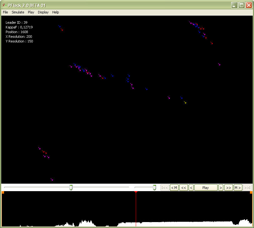
Figure 1. Snapshot of a P-Flock simulation with 50 agents, showing their positions and headings in a toroidal world. At time unit 1,600, a loose flock emerged; the program detected a possible leader (agent 39, shown in yellow). Agents with different perceptual features (see below) are displayed using different colours. A flocking index time series is displayed in the bottom section (see below). World and Agents
- 2.2
- The agents move in a two-dimensional, discrete world that is either toroidal or closed. The world is composed of cells or patches, and one cell can be occupied by only one agent at a time. Each agent i is identified by its coordinates (xi(t), yi(t)) and heading αi(t) at time t. The heading of an agent at time t is defined as the vector connecting its location at t-1 with its location at t, and is expressed as the anti-clockwise angle between that vector and the X axis, αi(t) = tan-1 [ (yi(t) - yi(t-1)) / (xi(t) - xi(t-1))].
- 2.3
- Agents have a perceptual field, which is defined as a circular sector whose centre is the agent's current location and which is bisected by its current heading vector; radius ri and angle θi of the circular sector are the depth and scope of agent i's perceptual field, respectively, and are the model parameters that can be modified (see Figure 2). Agent movement is restricted to its current local neighbourhood of cells; Moore or Von Neumann neighbourhoods can be defined with several possible diameters (see Figure 3).
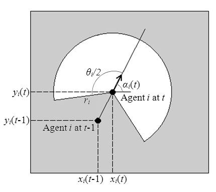
Figure 2. An agent's coordinates at times t-1 and t, its heading αi(t), and its perceptual field (in white), defined by radius ri and angle θi. 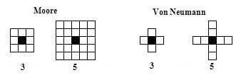
Figure 3. Moore and Von Neumann neighbourhoods and possible diameters. The agent's current position is indicated by a black square, and its current movement is limited by its neighbourhood. Ideal Distances and Dissatisfaction
- 2.4
- A matrix of ideal distances among the agents is also defined. The ideal distance from agent i to agent j at t, Dij(t), is the distance at which agent i wants to be from agent j at that time; ideal distances are not necessarily symmetrical. As agents encounter other agents, their ideal distances can change as a function of the outcome of their interaction. Agents' local goal is to minimize their dissatisfaction and to that end they can move within their current neighbourhood; an agent's dissatisfaction at time t, Ui(t), is defined as a composite function of the absolute differences between its ideal distance from every other agent that it currently perceives and the real distance from them:
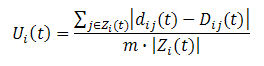
(1) where dij(t) is the Euclidean distance from agent i to agent j at t,
dij(t) = [(xi(t) - xj(t))2 + (yi(t) - yj(t))2]1/2 (2) and the sum is for all the agents currently perceived by agent i at t (subset Zi(t)). The sum is divided by the diameter of the world, or the maximum possible real distance (m), and by the cardinal number of Zi(t); dissatisfaction therefore has to be between 0 and 1 (for details, see Quera, Beltran, Solanas, Salafranca & Herrando 2000). The maximum possible real distance is a function of the size and shape of the world; for a rectangular world of size H × V, m = [H2 + V2]1/2 if it is non toroidal, and m = ([H2 + V2]1/2)/2 if it is toroidal.
- 2.5
- At time t, agent i estimates its ideal or possible future dissatisfaction for time t+1 for all candidate positions p within its current neighbourhood, by computing the distances from them to the current positions of the agents it is perceiving:
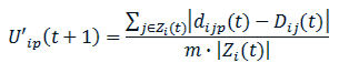
(3) where dijp(t) is the real distance from position p within agent i's neighbourhood to agent j's position at time t (see Figure 4). Agent i then decides to move to that position within its neighbourhood for which it estimated U'ip(t+1) to be the lowest value. If several positions share the minimum ideal dissatisfaction, the agent decides on the move that requires the least change to its current heading. At time t+1, the other agents could also have moved, and therefore the ideal dissatisfaction that agent i estimated for time t+1 might not necessarily have been attained. At each time unit the agents make the decision to move within their respective neighbourhoods simultaneously and independently. However, if two or more neighbourhoods overlap, then some of the cells in those neighbourhoods can be candidates for more than one agent if they happen to provide the minimum dissatisfaction for all of them. At each time unit, agents' priorities to move are sorted randomly. The agents with lower priorities will then only be able to move to those cells not chosen by agents with higher priorities that provide less than the minimum dissatisfaction.
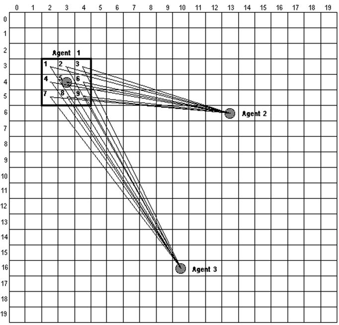
Figure 4. How an agent estimates its possible dissatisfaction at a given time. For every candidate position within its current neighbourhood (in this example, a Moore neighbourhood with a diameter of 3 and nine candidate positions), agent 1 computes the real distances from itself to the current positions of the other agents it perceives. These real distances are compared with the ideal distances as per the Equation 3 and a dissatisfaction is obtained for each candidate position. Flock Synthesis Rules
- 2.6
- In this model, ideal distances between agents vary as a consequence of the outcomes of their interactions, according to a set of reward rules, which we call Flock Synthesis Rules (FSRs) because a flock may emerge when they are applied locally, massively and repeatedly. Initially, agent i moves at random without considering any other agents; when it perceives agent j for the first time and their real distance apart is less than or equal to a critical value, PD, the FSRs for agent i are activated with regard to agent j, and the ideal distance from agent i to agent j is set so it is equal to a uniform random value between dij, their current real distance apart, and m, the maximum possible real distance. From that time on, ideal distance Dij undergoes two different kinds of change: smooth change and abrupt change.
- 2.7
- A smooth change is caused by agent i when it adapts to agent j's movements. As mentioned above, at each time step, agents i and j move to the positions in their respective current neighbourhoods that minimize their dissatisfaction. Before moving (time t-1), agent i predicted that its real distance from agent j at time t would be d'ij(t), assuming that agent j would not move. After moving, agent i evaluates the difference between its prediction, d'ij(t), and its previous real distance from agent j, dij(t-1):
cij(t) = d'ij(t) - dij(t-1) (4) - 2.8
- From the point of view of agent i, its movement was an "attempt to approach" agent j if cij(t) < 0, or an "attempt to move away" from agent j if cij(t) > 0. After moving, agent i also evaluates the discrepancies between the current real distance, dij(t), the predicted distance, d'ij(t), and the ideal distance it wanted to keep from agent j, Dij(t-1):
uij(t) = |dij(t) - Dij(t-1) | - | d'ij(t) - Dij(t-1) | (5) which is in fact the difference between the two partial dissatisfactions for agent i with respect to agent j: the actual one and the one it predicted it would have before moving. If uij(t) = 0, we can say that agent i has momentarily adapted to agent j, because the dissatisfaction it expected is fulfilled; if uij(t) < 0, agent i "overadapted" to agent j, because the dissatisfaction after moving is less than expected; and if uij(t) > 0, agent i "underadapted" to agent j, because the dissatisfaction after moving is greater than expected.
- 2.9
- The ideal distance from agent i to agent j is increased if agent i either attempted to approach and underadapted (cij(t) < 0 and uij(t) > 0) or attempted to move away and overadapted (cij(t) > 0 and uij(t) < 0); in the first case, increasing the ideal distance can be seen as a penalty, as the attempted approach was excessive, while in the second case, it can be seen as a reward, as the attempted move away was successful. On the other hand, the ideal distance is decreased if agent i either attempted to approach and overadapted (cij(t) < 0 and uij(t) < 0) or attempted to move away and underadapted (cij(t) > 0 and uij(t) > 0); in the first case, decreasing the ideal distance can be seen as a reward, as the attempted approach was successful, while in the second case, it can be seen as a penalty, as the attempted move away was excessive. Finally, the ideal distance either remains the same if agent i momentarily adapted (uij(t) = 0), or it is randomly increased or decreased if agent i overadapted or underadapted but attempted neither to approach or move away (cij(t) = 0 and uij(t) ≠ 0). Change in the ideal distance at time t is thus:
Dij(t) = (1 + kPC)Dij(t-1) (6) where PC is a parameter of the model that modulates the rate of change (0 < PC < 1), and k = +1, 0, or -1, for increase, no change and decrease, respectively (see Table 1 and Figure 5).
Table 1: Decision Table for the Flock Synthesis Rules Underadapted
uij(t) > 0Adapted
uij(t) = 0Overadapted
uij(t) < 0Attempt to approach
cij(t) < 0Increase (k = 1)
PenaltyNo change (k = 0) Decrease (k = -1)
RewardNo attempted move
cij(t) = 0Random
Increase or DecreaseNo change (k = 0) Random
Increase or DecreaseAttempt to move away
cij(t) > 0Decrease (k = -1)
PenaltyNo change (k = 0) Increase (k = 1)
Reward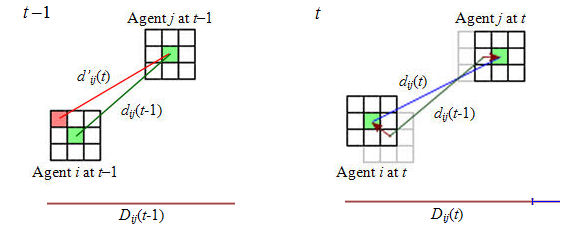
Figure 5. An example of agent i adapting to agent j and updating its ideal distance. The agents' positions are indicated by green cells at the centre of their current diameter-3 Moore neighbourhoods. At time t-1, agent i decided to move to the upper left cell in its neighbourhood because it happened to provide minimum dissatisfaction; agent i computed its real distance to agent j, dij(t-1) (shown in green), and the distance it predicted for time t, assuming that agent j would not move, d'ij(t) (shown in red). At time t, both agents moved (as indicated by the brown arrows, which are the agents' current headings) and the real distance between them is dij(t) (shown in blue). Agent i's ideal distance to agent j at t-1, Dij(t-1), is shown in brown. As cij(t) = d'ij(t) - dij(t-1) > 0, agent i attempted to move away from agent j. As |dij(t) - Dij(t-1)| < | d'ij(t) - Dij(t-1)|, uij(t) < 0, and agent i (slightly) overadapted to agent j when it moved. Consequently, agent i's movement with respect to agent j is rewarded and the ideal distance is increased by factor PC. - 2.10
- An abrupt change in the ideal distance from agent i to agent j occurs when that distance remains constant or changes cyclically in small amounts at consecutive time steps for a certain period of time Sij(T), T being the number of times the abrupt change occurred. This reflects agent i's tolerance towards being 'stagnated' with respect to agent j, i.e. remaining stable or relatively stable with respect to it. Initially, Sij(1) = PS, which is a parameter of the model. When the tolerance limit is reached, the ideal distance is increased abruptly by a factor equal to PC · Sij(T), i.e.
Dij(t) = Dij(t-1) + PCSij(T) (7) and it remains constant for the next Eij(T) time units, where Eij(T) is agent i's tolerance for being 'exiled' from agent j and T is the number of times the exile occurred. Initially, Eij(1) = PE, which is a parameter of the model. By increasing agent i's ideal distance from agent j abruptly when it stagnates, agent i is given an opportunity to adapt to new situations while it is exiled from agent j. When the exile time is over, the ideal distance is decreased abruptly by a factor equal to PC · Sij(T) + PD, i.e.
Dij(t) = Dij(t-1) - (PCSij(T) + PD) (8) and agent i resumes the smooth change phase with respect to agent j. Every time T that agent i is exiled with respect to agent j, its tolerance to stagnation is increased slightly by factor PC:
Sij(T) = (1 + PC)Sij(T - 1) (9) and every time it resumes the smooth change phase, its tolerance to exile is decreased slightly by that same factor:
Eij(T) = (1 - PC)Eij(T - 1) (10) - 2.11
- Thus, agent i progressively adapts to agent j by tolerating longer stagnation and shorter exile periods from it. The model parameters are listed in Table 2.
Table 2: Parameters of the Flock Synthesis Rules PD Critical real distance at which the FSRs are activated PC Change rate (0 < PC < 1) for increasing and decreasing ideal distances, and stagnation and exile tolerance times PS Initial value of the stagnation tolerance time PE Initial value of the exile tolerance time - 2.12
- It should be noted that the model does not require every agent to interact with every other agent. That is, whenever agent i perceives agent j, only the FSRs for i towards j are activated. Agent j may never have perceived i, or certain pairs of agents may never have perceived each other. Thus, repeated application of the dyadic FSRs make the group move in a coordinated way, even if some, or many, of the agents never interacted with each other. We must stress that, even if an agent perceives several agents simultaneously, the FSRs are applied in a dyadic and independent way. That is, if at time t agent i perceives agents j1, j2, and j3, the FSRs are independently applied three times, for agent i towards j1, j2, and j3, respectively; the decision for agent i towards j1 resulting from Table 1 has no effect on the decision for agent i towards j2, and so on.
- 2.13
- The pseudocode of the main functions of the P-Flock program is shown in the Appendix. The C code includes specific functions (not shown there) for computing Euclidean distances on a toroidal surface and agent dissatisfaction, and for checking which agents perceive other agents at every simulation step. The program reads a parameters file, performs the simulations, and saves the agents' coordinates, headings, ideal distances, and flocking and leadership indices (see below) to a text file. The simulation can then be played, paused, slowed down and played backwards (e.g. Figure 1). P-Flock 2.0 runs on Windows and can be downloaded from http://www.ub.edu/gcai/ (go to download in the main menu). A demo video can also be downloaded from that web site.
Quantifying Flocking
- 3.1
- When flocking behaviour is studied using agent-based simulation, flock detection is sometimes carried out merely by observing the changes in the agents' locations over time on the computer screen. Although some indicators are used to analyse flock behaviour (Kunz & Hemelrijk 2003; Parrish & Viscido 2005), there is no simple index that includes the different factors that indicate the degree of flocking behaviour as a whole and that is easily applicable to agent-based simulations (Zaera, Cliff & Bruten 1996).
- 3.2
- Therefore, in order to objectively describe flocking behaviour, we defined an index of the degree to which a set of agents actually formed a flock. A moving group as a whole was considered a flock when all the agents had similar headings and the distance between them was short enough (Quera, Herrando, Beltran, Salas & Miñano 2007). Given two agents, i and j, we defined their dyadic flocking index as the product of H, a function of the difference between the agents' headings, and Z, a function of their distance apart:
fij(t) = H(Δαij(t)) Z(dij(t)) (11) where Δαij(t) is the difference in radians between their headings,
Δαij(t) = min(|αi(t) - αj(t)|, 2π - |αi(t) - αj(t)|) (12) and dij(t) is the real distance between their locations at t. Functions H and Z are defined as:
H(Δαij(t)) = 1 - Δαij(t)/π (13) Z(dij(t)) = 1 - 1/[1 + exp(-g(dij(t) - rm)/m)] (14) Both functions can yield values between 0 and 1. Function H is equal to 1 when the agents' headings are identical, i.e. Δαij(t) = 0, and is equal to 0 when the two agents are facing opposite directions, i.e. Δαij(t) = π. Function Z is the inverse logistic function (with some parameters, g > 0, 0 < r < 1, m > 0); it tends towards 1 when the distance between the two agents is close to 0 (in which case the exponential function yields a high value), and it tends towards 0 when the distance is great (in which case the exponential function yields a value close to 0). Therefore, the more the agents face similar directions and the closer they are (i.e. when both H and Z approach 1), the greater their dyadic flocking index is; on the other hand, if the two agents have identical headings but are far away from each other, or if they are close to each other but their headings are opposite (i.e. either H or Z approach 0), their dyadic flocking index is low.
- 3.3
- A global flocking index for the N agents was defined as the arithmetic mean of the dyadic indices:
F(t) = [Σi<j fij(t)] / [N(N-1)/2] (15) Values of F(t) range from 0 to 1; when F(t) = 1, the group of agents move in a coordinated, compact fashion in the same direction, and when F(t) = 0, they are scattered and move in a disorderly fashion. Values of F(t) are a time series that indicates when the agents move as a flock and whether the flock is maintained over time. If the agents' behaviour is governed by some rules that make the flock emerge from initial disorderly movement, then an abrupt increase in F(t) indicates such a phase transition.
- 3.4
- Yet a group of agents moving randomly and not in a coordinated way can theoretically result in F(t) > 0. Therefore, in order to evaluate F(t) appropriately, we need to know the distribution function of the index for specific N, m, g, and r values in case the agents had random locations and headings. The distribution function can be estimated by assigning random coordinates and headings to the N agents repeatedly and independently many times (say, 10,000 times), and by calculating F for each one; by averaging the Fs, an estimate of their mathematical expectancy (E[F]) can be obtained. However, actual values of F(t) depend on the number of agents and the diameter of the world in which they move; therefore, in order to compare flocks with different group and world diameters, those indices must be converted into a common, or standardized, value. Cohen's (1960) kappa coefficient provides a way to compare an observed proportion of agreement with the proportion that is expected under the hypothesis of chance agreement, by calculating the ratio of the difference between observed and expected to the maximum possible difference. As F(t) and E[F] are observed and expected proportions, the same rationale as that used for calculating kappa can be applied in order to calculate the desired standardized index. Thus, the F(t) index can be converted into a kappa-like coefficient,
ΚF(t) = (F(t) - E[F])/(1 - E[F]). This index can be viewed as the degree to which agent interaction actually caused a flock to emerge: a flock exists when ΚF(t) > 0 (i.e. the agents' headings are similar and their distances apart are shorter than in the random case), and the closer ΚF(t) is to 1, the more defined the flock is (i.e. the more similar the agents' headings are and the shorter the distance between them). Figure 6 shows an example of series ΚF(t) for a simulation with 20 agents.
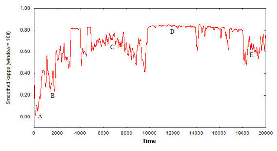
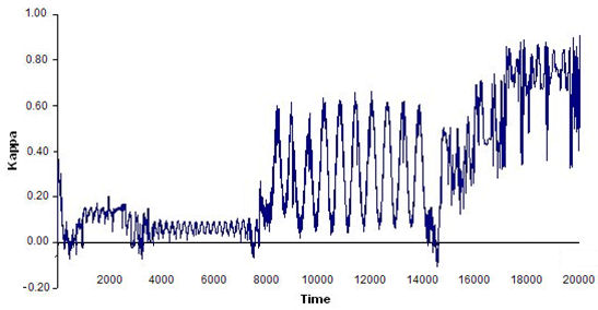
Figure 6a. Index ΚF(t) for a simulation with 20,000 time units and 20 agents for a specific combination of FSR parameters. 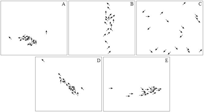
Figure 6b. Five snapshots are shown for specific moments of the simulation in Figure 6a: (A) movement is not coordinated, no flock exists; (B) a scattered flock begins to emerge from approximately time units 1,000 to 3,000, but is not maintained for long; (C) after two short periods of stable flocks before and after time unit 4,000, a period of instability follows; (D) after time unit 10,000, a compact, stable flock emerges and is maintained until time unit 18,000, with some oscillations mainly at time units 14,000 and 17,000, approximately; (E) a period of compact but unstable flocks follows, similar to period C. The index values have been smoothed out using a moving average window 100 time units wide.
An Index of Hierarchical Flock Leadership
- 4.1
- When a flock emerges (i.e. when ΚF(t) approaches 1), certain agents appear to lead the group. For an external observer, a leader agent is at one end with respect to the group and tends to face a direction opposite that of the group centroid, while the agents being led face the leader. By borrowing concepts and terminology from social network analysis (e.g. Faust & Waserman 1992; Waserman & Faust 1994), we defined a leadership index based on the amount of directed paths each agent received from the other agents. At time t, a sociomatrix M(t) = {mij(t)}, N × N, was defined as mij(t) = 1 if agent j was perceived by agent i, and j was not behind i; as mij(t) = 0 if agent j was not perceived by agent i, or j was behind i; or as mii(t) = 0. The sociomatrix can be represented by a directed graph or network in which each agent is a node, and an arrow connects i to j if mij(t) = 1. For agent j, its column and row sums of the sociomatrix at t (m+j(t) and mj+(t), respectively) are its nodal indegree and nodal outdegree. The former is agent j's degree prestige at t.
- 4.2
- However, it can be assumed that agents in a flock do not necessarily perceive all the other agents except for the immediate neighbours in front of them. When a leader agent exists, it may not necessarily be perceived and followed by the rest of agents, but only by a small fraction of them, which in turn are perceived and followed by other agents, and so on. Therefore, the leader agent does not necessarily have the highest nodal indegree (i.e. having a high degree prestige is not a necessary condition for being a leader). On the other hand, while the leader agent does not perceive any other agents in front of it and its nodal outdegree is consequently zero, non-leader agents may have nodal outdegrees equal to zero as well (i.e. having a null nodal outdegree is not enough to be a leader).
- 4.3
- An appropriate way of quantifying leadership is rank prestige: an agent's rank prestige is a function of the rank prestige values of the agents that target it, so that an agent targeted by many high-ranking agents has a higher prestige than one that is only targeted by low-ranking agents (Faust & Waserman 1992; Katz 1953; Seeley 1949). Therefore, an agent's leadership rank can be defined hierarchically as a function of the leadership ranks of the agents that perceive and follow it (a formal definition of hierarchical leadership is given by Shen 2007). Accordingly, agent j's rank Lj was defined as a linear combination of the ranks of those agents that perceive it:
Lj= m1jL1 + m2jL2 + ... + mNjLN= Σk=1..N mkjLk (16) In matrix notation, L = MTL, where L is the Nx1 vector of ranks, and MT is the transposed sociomatrix. The ranks are thus N unknowns in a linear system of N equations. Through diagonalization of MT, the elements of the eigenvector associated to its largest eigenvalue are the solution for that equation (Katz 1953).
- 4.4
- However, the ranks can also be obtained by means of this series (e.g. Foster, Muth, Potterat & Rothemberg 2001):
L = XU + X2U + X3U + X4U + ... (17) where X = aMT, U is an N × 1 vector of 1's, and a is an "attenuation factor" (0 < a < 1; Katz 1953) that ensures convergence of the series. That is, the transposed sociomatrix (multiplied by the attenuation factor) is raised to successive powers, and its rows are summed; finally, ranks are obtained by adding the row sums. As the powers increase, smaller values are obtained and the sum converges, provided that a < 1/maxi,j(mi+, m+j). Instead of raising the transposed sociomatrix to successive powers, Foster et al. propose estimating ranks by means of an iterative and computationally less complex procedure, which is appropriate for large N values.
- 4.5
- In fact, Equation 17 results from viewing ranks as the number of directed paths in the network from one agent to another and applying Markov chain theory (e.g. Manning, Raghavan & Schütze 2008, p. 425). While matrix M indicates the number of one-step paths from each agent to every other agent, cells in its squared matrix M2 contain the number of two-step paths from each agent to every other agent, irrespective of the intermediate one; in general, cells in matrix Mn contain the number of n-step paths connecting the agents, irrespective of the intermediate n-1 agents. By raising the sociomatrix to successive integer powers up to N, the total number of agents, and summing the columns of the resulting matrices (i.e. by applying Equation 17 up to the first N terms, and with X = MT), the total number of directed paths with one-, two-, …, and N-steps connecting any agent to each agent j are obtained.
- 4.6
- Still, sociomatrix M could contain loops or circular paths consisting of two or more steps; for example, agent i perceives agent j, which perceives agent k, which in turn perceives agent i. In that case, when M is raised to successive powers, column sums tend to increase exponentially. One solution is to substitute X = aMT, as mentioned. For the specific purpose of obtaining flock leadership indices, an alternative solution is to substitute X = (M ° F)T instead, where F = {fij(t)}, the symmetrical matrix of dyadic flocking indices, and ° stands for a Hadamard or entry-wise product; as M is binary and the dyadic flocking indices have to be between 0 and 1, this results in attenuation of loop effects and convergence of the series. We therefore proposed calculating leadership indices or ranks for a group of N agents as:
L = Σk=1 … N[(M ° F)T]kU (18) By using dyadic flocking indices as weights, the leadership indices reflect the degree of coordinated movement of the flock as well. When the flock is compact and all agent headings are very similar, many dyadic flocking indices are close to 1, and the resulting leadership indices are high (i.e. an agent leading a very compact and coordinated flock is a "strong" leader); on the other hand, when the flock is scattered or there is substantial variability of agent headings, few dyadic flocking indices are close to 1, and the resulting leadership indices are low (i.e. an agent leading a not-so-compact or coordinated flock is a "weak" leader).
- 4.7
- It should be noted that hierarchical leadership, as it is defined here, is different from effective leadership (Couzin, Krause, Franks & Levin 2005). Effective leadership is defined in terms of information transfer among individuals, and "can emerge as a function of information differences among members of a population" (p. 515). Therefore, while effective leadership explains group motion, hierarchical leadership is simply a description made by an external observer. Calling an agent a hierarchical leader is not an explanation of why a group moves coordinately as it does; instead, what explains coordinated motion is the mechanism governing the agents' interaction, that is, the FSRs.
An Example
- 4.8
- Figure 7 shows a snapshot of N = 8 agents as they move in two-dimensional space. Short blue arrows indicate their current headings. A network of red arrows connecting agents indicate which agents perceive other agents in front of them. In the upper left corner of the figure there is a schematic representation of the scope and depth of the agents' perception field; agents' coordinates and headings in radians are shown in Table 3.
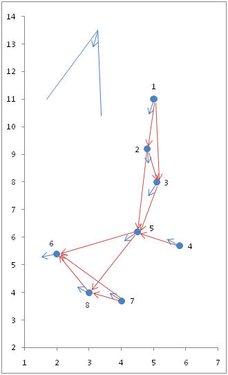
Figure 7. A snapshot of 8 agents as they move in two-dimensional space, indicating their headings and the perception network.
For this network, sociomatrix M and dyadic flocking indices F are shown in Tables 4a and 4b, respectively. Finally, Table 4c shows the results of [(M ° F)T]kU, for powers k = 1 to 8, plus the leadership indices. As visual inspection of Figure 7 suggests, agent 6 is the leader; accordingly, its leadership index is the highest. It should be noted that in this case agent 6 was the only agent with a null outdegree, and that agents 5 and 6 share the highest indegree.Table 3: Headings (in radians) and two-dimensional coordinates of a group of 8 agents Agent Heading X Y 1 4.54 5.0 11.0 2 4.75 4.8 9.2 3 4.01 5.1 8.0 4 2.79 5.8 5.7 5 3.49 4.5 6.2 6 3.32 2.0 5.4 7 2.97 4.0 3.7 8 2.97 3.0 4.0 Table 4a: Sociomatrix for the 8 agents shown in Figure 7 (matrix M) Agents 1 2 3 4 5 6 7 8 Out Agents 1 0 1 1 0 0 0 0 0 2 2 0 0 1 0 1 0 0 0 2 3 0 0 0 0 1 0 0 0 1 4 0 0 0 0 1 0 0 0 1 5 0 0 0 0 0 1 0 1 2 6 0 0 0 0 0 0 0 0 0 7 0 0 0 0 0 1 0 1 2 8 0 0 0 0 0 1 0 0 1 In 0 1 2 0 3 3 0 2 Table 4b: Dyadic flocking indices for the 8 agents shown in Figure 7 (matrix F) Agents 1 2 3 4 5 6 7 8 Agents 1 1.000 0.933 0.833 0.444 0.667 0.611 0.500 0.500 2 0.933 1.000 0.767 0.378 0.600 0.544 0.433 0.433 3 0.833 0.767 1.000 0.611 0.833 0.778 0.667 0.667 4 0.444 0.378 0.611 1.000 0.778 0.833 0.944 0.944 5 0.667 0.600 0.833 0.778 1.000 0.944 0.833 0.833 6 0.611 0.544 0.778 0.833 0.944 1.000 0.889 0.889 7 0.500 0.433 0.667 0.944 0.833 0.889 1.000 1.000 8 0.500 0.433 0.667 0.944 0.833 0.889 1.000 1.000 Table 4c: Results of applying Equation 18, for powers k = 1 to 8, and leadership indices for the agents Agents 1 2 3 4 5 6 7 8 Powers 1 0 0.933 1.600 0 2.211 2.722 0 1.833 2 0 0 0.716 0 1.893 3.718 0 1.843 3 0 0 0 0 0.596 3.426 0 1.578 4 0 0 0 0 0 1.966 0 0.497 5 0 0 0 0 0 0.442 0 0.833 6 0 0 0 0 0 0 0 0 7 0 0 0 0 0 0 0 0 8 0 0 0 0 0 0 0 0 Lj 0 0.933 2.316 0 4.701 12.273 0 5.751
Method
- 5.1
- We ran two series of simulations with P-Flock. With the first series we tried to identify the environmental conditions (size of the universe), agent features (perceptual depth and scope) and values for the FSR parameters that made compact flocks emerge, and analysed how the flocking indices behaved in the time steps prior to flock emergence. With the second series of simulations we detected the agents that had become flock leaders and tried to determine whether an agent's initial spatial position (central vs. peripheral) could be used to predict its chances of becoming a future leader.
Flock Emergence
- 5.2
- In the first simulation series, eight different toroidal world sizes were explored (600 × 450, 260 × 200, 230 × 180, 210 × 180, 200 × 150, 180 × 150, 150 × 120, and 120 × 90). Previous work had indicated that certain values of agent features and FSR parameters could favour flock emergence (Quera, Herrando, Beltran, Salas & Miñano 2007). The number of agents was therefore set at 20 and their perceptual scope and depth were set at 3π/2 and 60, respectively, for all simulations. A Moore agent neighbourhood with a diameter of 3 was used. The initial agent positions were assigned and equally spaced, like nodes on a grid, and the agent headings were set so they were identical and equal to π/4. The FSR parameters were PD = 60, PC = 0.01, and PS = PE = 6. For each simulation (with a specific world size), P-Flock was run for 20,000 time steps. For each world size, the simulation was replicated four times. At each time step t, the program calculated flocking index ΚF(t).
- 5.3
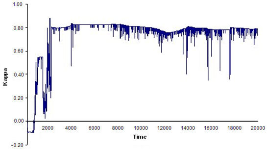
- The results showed that the bigger the world was, the more difficult it was for a flock to emerge, as agents that were more scattered tended to take longer to begin interacting with one another. Conversely, the smaller the world, the less stable the flocks were that emerged, as the amount of interaction among the agents increased and they were more likely to change continuously in a small world, which led to flocks that emerged and disbanded often. The optimal world size for flock emergence was found to be 150 × 120. Figure 8 shows four examples of time series of index ΚF(t) for various world sizes.
(a) 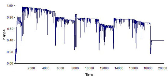
(b) 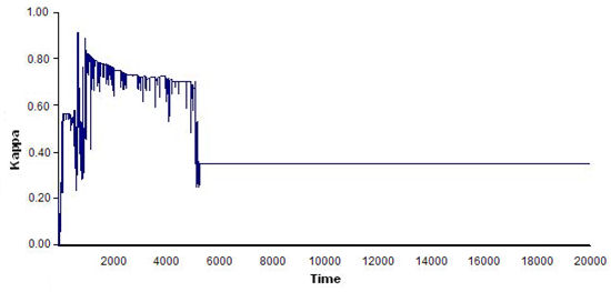
(c) 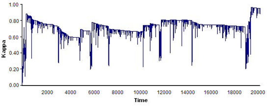
(d) Figure 8. Four examples of time series of index ΚF(t) for different world sizes: (a) 600 × 450, flocks were very unstable; (b) 230 × 180, flocks formed early but tended to disband in the long run; (c)120 × 90; flocks formed early but then disbanded; and (d) 150 × 120, flocks remained for a long period of time. See text for details on model parameters and agent features. - 5.4
- Previous work also revealed that the agents' perceptual depth and scope were critical to producing flock emergence (Quera, Herrando, Beltran, Salas & Miñano 2007). We therefore ran a new series of simulations to determine the combinations of perceptual depth and scope that were optimal for generating flocks. We kept the toroidal world size constant at 150 × 120 and the number of agents constant at 20. The FSR parameters were the same as in previous simulations. As we had done previously, the agents' initial positions were assigned and equally spaced. Their headings were set at π/4. The following combinations of the perceptual parameters were tried: (depth 40, scope 6π/4), (60, 6π/4), (80, 6π/4), (60, 5π/4), (80, 5π/4), and (60, 7π/4). For each combination, P-Flock was run for 20,000 time steps, and flocking indices were calculated at each t; each simulation was replicated four times. The results showed that the most compact, stable flocks were formed at (60, 6π/4) and (80, 5π/4). Two new simulations, with four replications each, were run by assigning initial positions and headings randomly and uniformly, and trying the combination of perceptual parameters again (60, 6π/4) and (80, 5π/4); the latter showing the most compact, stable flocks (i.e. high perceptual distance and low scope).
- 5.5
- A new series of simulations was run in order to identify the FSR parameters that favoured flock emergence and maintenance by keeping all the other parameters constant (toroidal world size 150 × 120; perceptual depth and scope 80 and 5π/4, respectively; 20 agents with random initial coordinates and headings), and exploring several combinations of parameters PD, PC, and PS (parameter PE was set equal to PS). First, the following combinations of values for the FSR parameters were tried: (PD = 6, PC = 0.01, PS = 6), (100, 0.01, 6), (6, 0.01, 100), (6, 100, 6), and (100, 0.01, 100). For each combination, P-Flock was run for 20,000 time units and replicated four times; compact, stable flocks were produced when PD > 6. Next, while keeping PD = 60 and PC = 0.01 constant, new simulations were run (20,000 time units each, four replications) by varying PS = 5, 12, 15, 20, 22, 25, 40; compact, stable flocks were found when 5 < PS < 25. Finally, while keeping PD = 60 constant, the following combinations were tried: (PC = 0.02, PS = 6), (0.03, 6), (0.05, 6), (5, 6), (0.03, 25), and (0.05, 25); compact, stable flocks were obtained when PC < 0.02.
- 5.6
- Finally, we ran 100 simulations (20,000 time units and four replications each) using the optimal world and parameter values obtained in previous simulations. We set the FSR parameters at PD = 60, PC = 0.01, and PS = PE = 6, and assigned uniform random initial agent coordinates and headings. At each time step of the simulation, the program calculated flocking and leadership (L) indices. The results showed that compact, stable flocks emerged and were maintained in 72% of the simulations (see Figure 9).
(a) 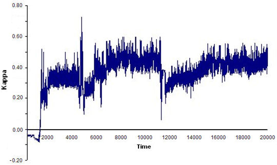
(b) Figure 9. Time series of index ΚF(t) for: (a) an example of a compact, stable flock, and (b) an example of a loose, unstable flock. Toroidal world size: 150 × 120; 20 agents; perceptual depth: 80; scope: 5π/4; and FSR parameters: PD = 60, PC = 0.01, PS = PE = 6. - 5.7
- For the simulations in which compact, stable flocks emerged, we searched for possible patterns in how the flocking index behaved during the time steps immediately prior to flock emergence. Figure 10 shows four examples with a zoom on the 100 time units prior to that point. No regular patterns were observed (i.e. no general growth model seemed reasonable), except for an abrupt increase in the flocking index (ranging between 0.3 and 0.5 in kappa units) approximately 20 time units prior to flock emergence.
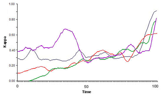
Figure 10. Four examples of the time series of index ΚF(t) in the 100 time units immediately prior to flock emergence. Note that there was a sharp increase in approximately the last 20 time units. Flock Leadership
- 5.8
- P-Flock computed a leadership index for each agent at each time unit. The agent with the highest leadership index Lj at time t could be considered the momentary leader. Leadership was dubious if ΚF(t) was low, say, less than 0.80; in that case, two or more groups of agents could have formed flocks independently, and thus the agent with the highest leadership index could not be viewed as the leader for the whole group. When leadership was not dubious, an agent with the highest Lj for a long period of time could be considered a stable leader. Stable leadership was mutually exclusive, i.e. there could only be one stable leader at a time. An example of stability of leadership is shown in Figure 11.
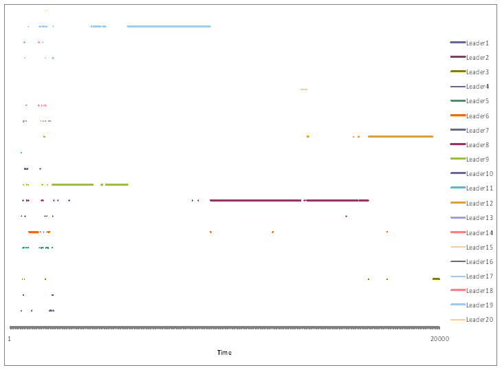
Figure 11. Time lines indicating leadership periods for a simulation with 20,000 time units. Each colour represents a different agent. Long segments indicate stable leaders. A succession of very short segments is shown at the beginning of the simulation representing an initial period when no stable flocks had formed yet. - 5.9
- The distribution of leadership time among the agents could indicate how stable or unstable the leaders were. A group with a single leader throughout the simulation would have had a totally skewed time distribution, with one agent monopolizing all the leadership time; conversely, a group whose agents took over as leaders successively and perhaps recurrently would have had a more uniform time distribution. We computed the distributions of leadership time for groups of 20 agents from the results of 100 simulations obtained previously (see section Flock Emergence). The simulations were divided into two sets: those that showed compact, stable flocks (72%) and those that showed unclear flocks (28%). For each simulation, the total leadership time of each agent was obtained and its unconditional probability was computed; the entropy of the time distribution was calculated using Shannon & Weaver's (1949) formula, H = - Σ pi log2(pi), where pi is agent i's unconditional probability of being a leader, and is estimated as the proportion of time the agent was the leader during the simulation. Entropy measures the degree of uncertainty (in bits). Thus, if an agent monopolized all the leadership time, H = 0 bits; conversely, if all the agents (N) in the group were leaders for exactly the same amount of time, entropy was the maximum, H = log2(N) bits. Average entropy for the first set of simulations (compact, stable flocks) was 2.835 bits (standard deviation 0.449 bits), and for the second set (loose, unstable flocks) was 3.224 bits (standard deviation 0.494 bits); maximum entropy was log2(20) = 4.322 bits. A two tailed t-test showed a significant difference between them (t = -3.62; p < 0.001; df = 46). Therefore, when flocks were compact and stable, their leaders tended to remain stable and monopolize the leadership time more than when flocks were loose and unstable, in which case leaders tended to change more often.
Centrality and Leadership
- 5.10
- Being in a centre position with respect to the other agents could have caused an agent to become a leader, as it could have been perceived as one by most other agents. In order to determine whether the emergence of a leader agent could be predicted from its initial location relative to the other agents, centrality at time 0 was computed for 298 agents that had shown stable leadership, i.e. whose leadership remained for long periods of time during the simulations.
- 5.11
- Agent centrality was calculated according to Mardia (1972): for each agent i, a unit vector towards every other agent j was computed at time 0, wij = (uij, vij), with coordinates uij = (xj - xi)/dij and vij = (yj - yi)/dij, where (xi, yi) and (xj, yj) are agent i's and j's coordinates at time 0, respectively, and dij is the distance between them. Agent i's centrality is thus the module of the sum of its unit vectors towards all the other agents, i.e. Gi =|Σi ≠ j wij|. The smaller the Gi, the more central agent i's location is in relation to the other agents. An example is shown in Figure 12 for a group of 8 agents. Unit vectors for two agents (green and yellow) and the sums of those vectors (in red) are displayed; because the green agent's location is more central than the yellow agent's, its unit vectors are more uniformly distributed, thus yielding a sum vector with a smaller module.
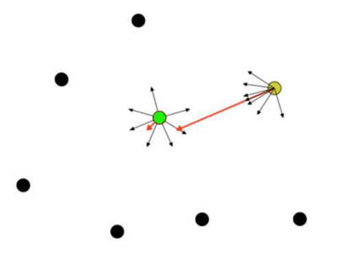
Figure 12. Centrality vectors (in red) for two agents in a group of eight - 5.12
- Figure 13 shows the number of stable leaders as a function of their initial centrality ranks, where rank 1 means maximum centrality, i.e. the smallest Gi; because the total number of agents was set at 20, agents with a centrality rank 20 were the most peripheral at the beginning of the simulations. For initial centrality to be a predictor of future leadership, the distribution of ranks had to be positively skewed, i.e. many stable leaders would have ranks of 1 or similar, and there would be progressively fewer stable leaders with ranks far above 1. However, as the figure indicates, initial centrality did not seem to be correlated with leadership. Agents that became stable leaders were located indistinctively in central and peripheral positions at the beginning of the simulations.
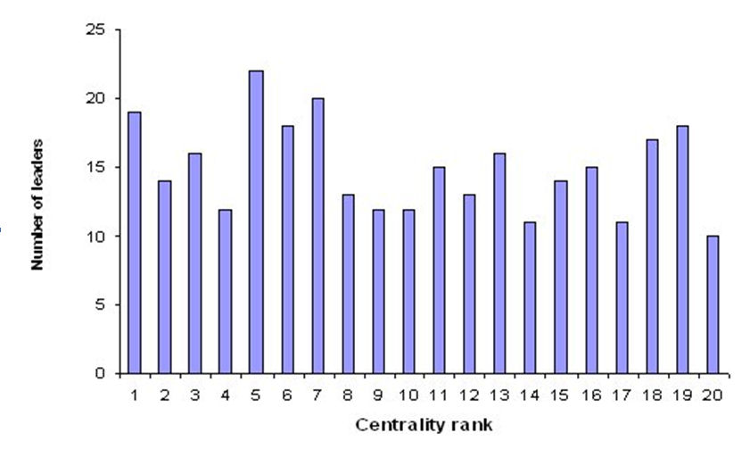
Figure 13. Number of stable leaders (N=298) as a function of their initial centrality ranks. Rank 1 means maximum centrality
Discussion and Conclusions
- 6.1
- Like a classic Reynolds model, our agent-based model made flocks emerge. Unlike it, our model did not assume that agents could perceive and evaluate distances and velocities for groups of neighbouring agents in order to match their movements. Instead, the Flocking Synthesis Rules only required each agent to adapt momentarily to the other agents it encountered, and adaptation was accomplished by rewarding and penalizing attempted approaches and movements away. Moreover, in our model agents tried to minimize their local dissatisfaction by moving to the positions in their local neighbourhood where they predicted that the differences between the real distances they kept from the currently perceived agents and the ideal distances they wanted to keep from them would be minimal. In turn, the ideal distances varied as a consequence of rewarding. Each agent tried to minimize its dissatisfaction independently, and therefore moving to a certain position where the minimum was predicted did not guarantee that it would be fulfilled, as neighbouring agents would have moved as well. Consequently, it was highly unlikely for all agents to reach an absolute minimum; that lack of equilibrium was what maintained the group in movement. Still, nothing in the FSRs indicated that the agents had to move in a coordinated fashion as a whole. Therefore, when, as a result of repeated dyadic interactions and applications of the FSRs, the group tended to move in the same direction in a compact way, we could say that a flock emerged from the local dyadic rules.
- 6.2
- The fact that, once a flock had emerged, certain agents tended to be at one end of the group for long periods of time and the rest of the agents seemed to "follow" them might prompt an external observer to label the former agents "leaders". Again, nothing in the FSRs specified that, depending on certain dyadic interactions, certain agents should become leaders, and therefore, leadership in our virtual flocks was also an emergent phenomenon.
- 6.3
- We developed a method for quantifying the degree to which a group of agents moved in a coordinated fashion (flocking index) and applied concepts from social networks in order to obtain the degree to which each individual agent was a leader. These indices were computed by our P-Flock program at each simulation step, thus providing time series that could be inspected to indicate when a flock emerged, whether it was maintained for short or long periods of time, and which agent had the highest leadership index and for how long. Leadership indices indicated where agents were located in the hierarchy of coordinated movement; the agent with the highest leadership index had all other agents behind it, while agents with lower indices had some subgroup of other agents behind them, and so on.
- 6.4
- Due to the great many possible agent, world and model parameter combinations, we could only explore some of them. Our aim was to determine which of them favoured flock emergence and then characterize stable agents. We first varied some world parameters and left agents' perceptual and model parameters constant; then, once an optimal world size was found, several combinations of perceptual parameters were explored, while keeping FSR parameters constant; finally, several combinations of FSR parameters were explored and the rest of parameters remained constant. Of course, this procedure did not guarantee that we would find the optimal combination for all parameters; a full factorial design including all of them, or a fractional factorial design including a subset of the more relevant parameters, would make that possible. Our results were therefore tentative and can be summarized as: (a) the bigger the world size, the more stable the flocks were once they emerged; (b) the most compact, stable flocks appeared when the agents' perceptual distance was large and their scope was small; (c) for the optimal combinations of parameters found, compact, stable flocks emerged and were maintained in 72% of the simulations.
- 6.5
- Finally, we explored how leaders behaved once stable flocks formed and found that: (a) when flocks were compact and stable, their leaders also tended to remain relatively stable and, although several agents could become absolute leaders one after another, they tended to monopolize the total leadership time more when flocks were compact and stable than when they were loose and unstable, in which case leaders tended to change more often; and (b) future leadership could not be predicted based on initial agent centrality, as agents in both central and peripheral positions at the beginning of the simulations eventually became stable leaders.
- 6.6
- Multi-agent simulation gives us a powerful tool to study the emergence of leaders in self-organized groups of individuals. Both the flock-inspired approach and multi-agent simulation provide a promising framework for future research on leaders and leadership. More simulation experiments with P-Flock are necessary to understand and characterize the emergence of stable leaders in flocks. Future developments will include a new version of the program for simulating flocks in three dimensional worlds and the validation of the model and the program by fitting it to empirical data from automatic tracking of individuals in fish schools, obtained in controlled laboratory experiments.
Acknowledgements
- This project was partially supported by grants from the Directorate General for Research of the Government of Catalonia (2005SGR-0098, 2009SGR-1492), from the Directorate General for Higher Education and Culture of the Spanish Government (SEJ2005-07310-C02-01/PSIC, PSI2009-09075) and from the European Union's ERDF program. The authors would like to thank Antoine Berlemont for his assistance running simulations and data analyses, Axel Guillaumet for developing the Windows viewer component for P-Flock 2.0, and two anonymous reviewers for their comments and suggestions on an earlier version of the manuscript.
Appendix
-
Pseudocode of the P-Flock program
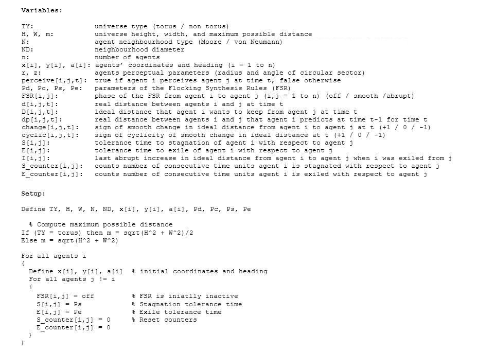
Figure A1. General variables and initial setup 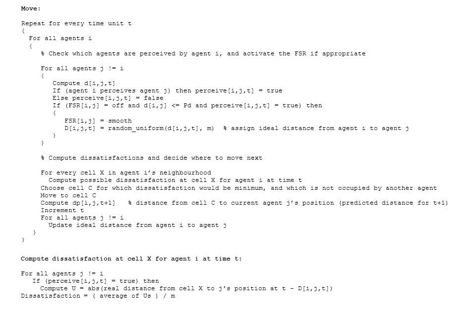
Figure A2. Agent movement and dissatisfaction 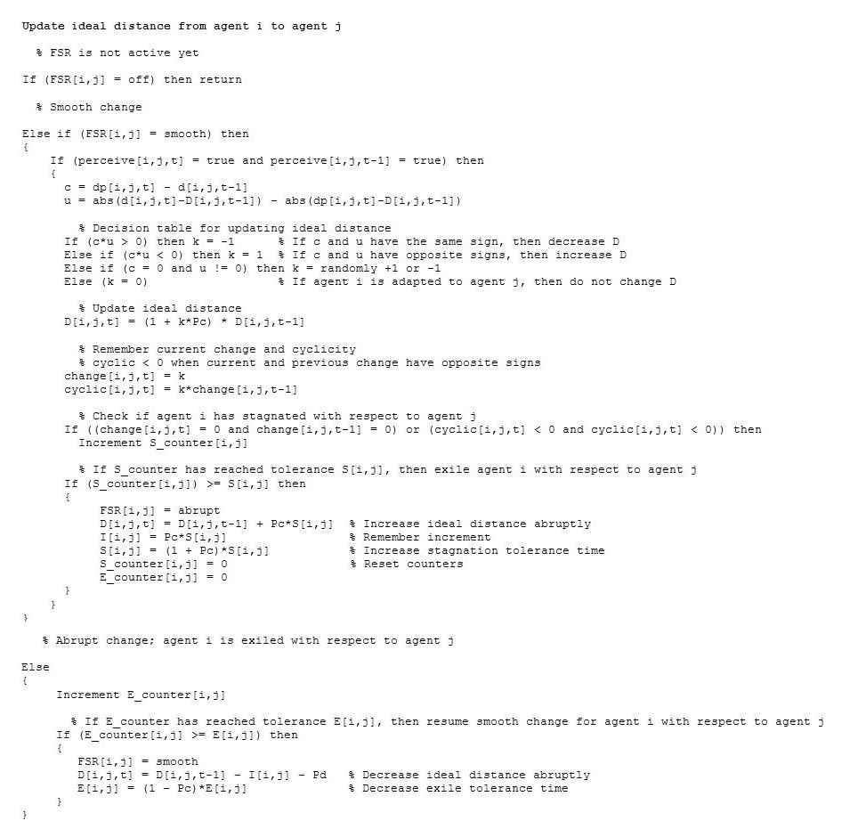
Figure A3. Updating of ideal distances according to the Flock Synthesis Rules
References
-
BALDASSARRE, G, Nolfi, S and Parisi, D (2002) Evolving mobile robots able to display collective behaviours. Artificial Life, 9, pp. 255-267. [doi:10.1162/106454603322392460]
BASS, B M (1990) Bass & Stodhill's Handbook of Leadership. New York: Free Press.
BARNAJEE, A B (1992) A simple model of herd behaviour. Quarterly Journal of Economics, 107 (3), pp. 797-17. [doi:10.2307/2118364]
BELTRAN, F S, Salas, L and Quera, V (2006) Spatial behavior in groups: An agent-based approach. Journal of Artificial Societies and Social Simulation, 9 (3) 5. https://www.jasss.org/9/3/5.html
CAVAGNA, A, Giardina, I, Orlandi, A, Parisi, G, Procaccini, A, Viale, M and Zdravkovic, V (2008) The STARFLAG handbook on collective animal behaviour: 1. Empirical methods. Animal Behaviour, 76, pp. 217-236. [doi:10.1016/j.anbehav.2008.02.002]
COHEN, J A (1960) A coefficient of agreement for nominal scales. Educational and Psychological Measurement, 20, pp. 37-46. [doi:10.1177/001316446002000104]
COUZIN, I D, Krause, J, Franks, N R and Levin, S A (2005) Effective leadership and decision-making in animal groups on the move. Nature, 433, pp. 513-516. [doi:10.1038/nature03236]
FAUST, K and Waserman, S (1992) Centrality and prestige: A review and synthesis. Journal of Quantitative Anthropology, 4, pp. 23-78.
FOSTER, K C, Muth, S Q, Potterat, J J and Rothenberg, R B (2001) A faster Katz status score algorithm. Computational & Mathematical Organization Theory, 7, pp. 275-285. [doi:10.1023/A:1013470632383]
HEDSTRÖM, P (1998) Rational imitation. In Hedström P and Swedberg R (Eds.) Social mechanisms:An analytical approach to social theory (pp. 306-327), Cambridge, UK: Cambridge University Press. [doi:10.1017/CBO9780511663901.012]
HEDSTRÖM, P (2005) Dissecting the social: On the principles of analytical sociology. Cambridge, UK: Cambridge University Press. [doi:10.1017/CBO9780511488801]
HEDSTRÖM, P and Swedberg, R (1998) Social mechanisms: An introductory essay. In Hedström P and Swedberg R (Eds.) Social mechanisms: An analytical approach to social theory (pp. 1-31), Cambridge, UK: Cambridge University Press. [doi:10.1017/CBO9780511663901.001]
HOUSE, R J (1977) A 1976 theory of charismatic leadership. In Hunt J G and Larson L L (Eds.) Leadership: The cutting edge (pp. 189-207), Carbondale, IL: Southern Illinois University Press.
KATZ, L (1953) A new status index derived from sociometric analysis. Psychometrika, 18, pp. 39-43. [doi:10.1007/BF02289026]
KIRKPATRICK, S A and Locke, E A (1991) Leaderships: Do traits matter? Academy of Management Executive, 5, pp. 48-60. [doi:10.5465/ame.1991.4274679]
KUNZ, H and Hemelrijk, C K (2003) Artificial fish schools: Collective effects of school size, body size and body form. Artificial Life, 9, pp. 237-253. [doi:10.1162/106454603322392451]
MANNING, C D, Raghavan, P and Schütze, H (2008) Introduction to information retrieval. New York: Cambridge University Press.
MARDIA, M K (1972) Statistics of directional data. London: Academic Press.
PARRISH, J K and Viscido, S V (2005) Traffic rules of fish schools: a review of agent-based approaches. In Hemelrijk C (Ed.) Self-organisation and evolution of social systems (pp. 50-80), Cambridge, UK: Cambridge University Press.
QUERA, V, Beltran, F S, Solanas, A, Salafranca, L and Herrando, S (2000) A dynamic model for inter-agent distances. In Meyer J-A, Berthoz, A, Floreano, D, Roitblat H L and Wilson S W (Eds.) From Animals to Animats 6 Proceedings Supplement (pp. 304-313), Honolulu, Hawaii: The International Society for Adaptive Behavior.
QUERA, V, Herrando, S, Beltran, F S, Salas, L and Miñano, M (2007) An index for quantifying flocking behavior. Perceptual and Motor Skills, 105, pp. 977-987. [doi:10.2466/pms.105.7.977-987]
QUERA, V, Solanas, A, Salafranca, Ll, Beltran, F S and Herrando, S (2000). P-SPACE: A program for simulating spatial behavior in small groups. Behavior Research Methods, Instruments and Computers, 31 (1), pp. 191-196. [doi:10.3758/BF03200801]
REYNOLDS, C W (1987) Flocks, herds and schools: A distributed behavioral model. Computer Graphics, 21 (4), pp. 25-34. [doi:10.1145/37402.37406]
ROSEN, D (2003) Flock theory: A new model of emergent self-organization in human interaction. Paper presented at the annual meeting of the International Communication Association, San Diego.
SEELEY, J R (1949) The net of reciprocal influence: A problem in treating sociometric data. Canadian Journal of Psychology, 3, pp. 234-240. [doi:10.1037/h0084096]
SHANNON, C Y and Weaver, W (1949) The mathematical theory of communication. Urbana, Ill.: The University of Illinois Press.
SHEN, J (2007) Cucker-Smale flocking under hierarchical leadership. SIAM Journal on Applied Mathematics, 68 (3), pp. 694-719. [doi:10.1137/060673254]
TURING, A (1950) Computing machinery and intelligence, Mind, 59 (236), pp. 433-460. [doi:10.1093/mind/LIX.236.433]
WASERMAN, S and Faust, K (1994) Social networks analysis. Methods and applications. Cambridge, UK: Cambridge University Press. [doi:10.1017/CBO9780511815478]
ZAERA, N, Cliff, C and Bruten, J (1996) (Not) evolving collective behaviours in synthetic fish. In Maes, P, Mataric, M J, Meyer, J-A, Pollack, A and Wilson, S W (Eds.) From animals to animats 4 (pp. 635-644), Cambridge, MA: MIT Press.