
 Abstract
- In this work simulation-based and analytical results on the emergence steady states in traffic-like interactions are presented and discussed. The objective of the paper is twofold: i) investigating the role of social conventions in coordination problem situations, and more specifically in congestion games; ii) comparing simulation-based and analytical results to figure out what these methodologies can tell us on the subject matter. Our main issue is that Agent-Based Modelling (ABM) and the Equation-Based Modelling (EBM) are not alternative, but in some circumstances complementary, and suggest some features distinguishing these two ways of modeling that go beyond the practical considerations provided by Parunak H.V.D., Robert Savit and Rick L. Riolo. Our model is based on the interaction of strategies of heterogeneous agents who have to cross a junction. In each junction there are only four inputs, each of which is passable only in the direction of the intersection and can be occupied only by an agent one at a time. The results generated by ABM simulations provide structured data for developing the analytical model through which generalizing the simulation results and make predictions. ABM simulations are artifacts that generate empirical data on the basis of the variables, properties, local rules and critical factors the modeler decides to implement into the model; in this way simulations allow generating controlled data, useful to test the theory and reduce the complexity, while EBM allows to close them, making thus possible to falsify them.
- Keywords:
- Agent-Based Modelling, Equation-Based Modelling, Congestion Game, Model of Social Phenomena
Introduction
- 1.1
- Ten years ago, during the first Multi-Agent Systems and Agent-Based Simulation Workshop (MABS '98), Parunak H.V.D., Robert Savit and Rick L. Riolo discussed the similarities and differences between the Agent-Based Modelling (ABM) and the Equation-Based Modelling (EBM), developing some criteria for selecting one or the other approach (Parunak et al. 1998). They claimed that despite sharing some common concerns, ABM and EBM differ in two ways: the fundamental relationships among the entities they model, and the level at which they operate. The authors observed that these two distinctions are tendencies, rather than hard and fast rules, and indicate that the two approaches can be usefully combined.
- 1.2
- During the last ten years, a lively debate on the subject matter has been developed (see Epstein 2007). An overall review is beyond the scope of this work. In this contribution, we will address a theoretical issue concerning the emergence of social conventions and we will explore how and to what extent an integrated approach of ABM and EBM methodologies can help us handle it. The aim of this work is to explore the emergence of steady states in congestion games (Rosenthal 1973; Milchtaich 1996; Chmura and Pitz 2007), and more specifically, to investigate the emergence of a precedence rule in traffic-like interactions (see also Sen and Airiau 2007).
- 1.3
- A congestion game is a game where each player's payoff is non-increasing over the number of other players choosing the same strategy. We use a Wikipedia example to show this concept:
for instance, a driver could take U.S. Route 101 or Interstate 280 from San Francisco to San Jose. While 101 is shorter, 280 is considered more scenic, so drivers might have different preferences between the two independent of the traffic flow. But each additional car on either route will slightly increase the drive time on that route, so additional traffic creates negative network externalities
- 1.4
- A celebrated congestion game is the Minority Game, where the only objective for all players is to be part of the smaller of two groups (Challet and Zhang1997, 1998; Chmura and Pitz 2006). A well-known example of the minority game is the El Farol Bar problem proposed by W. Brian Arthur (1994), in which a population of agents have to decide whether to go to the bar each week, using a predictor of the next attendance. All agents like to go to the bar unless it is too crowded (i.e. when more that 60% of the agents go). But since there is no single predictor that can work for everybody at the same time, there is no deductively rational solution. How can agents achieve this goal to go to the bar, avoiding crowd?
- 1.5
- It has been suggested that in coordination problem situations (like congestion games), a convention is a pareto-optimal rational choice (see Gilbert 1981; Lewis 1969; Sugden 2004; Young 1993), i.e. a choice in which any change to make any person better off is impossible without making someone else worse off, thereby in these kind of circumstances it should be the conventional solution to emerge.
- 1.6
- In this paper, we suggest a different solution to the subject matter, arguing that in specific coordination problem situations, more specifically in 4-strategy game structures, a conventional equilibrium is not granted to emerge. Thus, the objective of the paper is twofold: a) showing that in coordination problem situations, rational agents may also converge on non-conventional equilibriums; b) comparing and integrating simulation-based and analytical results in order to draw some conclusions about what these methodologies can tell us on the subject matter.
- 1.7
- The paper is divided into seven sections: sections 2 and 3 describe a general technique to write an analytic model for a population game (like a congestion game), i.e. the replicator-projector dynamic. In section 4 we describe our model and an algorithm to implement the replicator dynamic onto it. Our model is based on the interaction of strategies of heterogeneous agents who have to cross a junction trying to avoid collisions. In each junction there are only four inputs, each of which is passable only in the direction of the intersection and can be occupied only by an agent one at a time. The agents can perceive the presence of other agents only if they come from orthogonal directions. There are four types of agents, each characterized by a different strategy: two of these strategies consider binding on its decision the presence of other agents from a particular direction (e.g. by observing their right) to cross the junction. We call these strategies (and these agents) conditioned. In sections 5 and 6 we describe the results of simulation and analytic procedures. Finally, in section 7 we argument about the relationship between simulation and analytic results and we point out some possible outcomes.
 The replicator dynamics
- 2.1
- Congestion games involve large numbers of simple agents, each of them playing one out of a finite number of rules. In general, a congestion game deals with a society P of p different population of agents; nevertheless, our model will use only a single population (case p=1). We call these games population games. During the game, each agent chooses a strategy from the set S = {1,...,n}where n is the total number of strategies (behaviors). Now we will describe the replicator dynamics for population games.
- 2.2
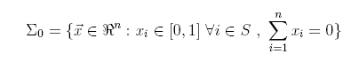
- Let Σ be the space containing all the vector of frequency distributions of the agents playing,
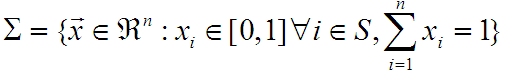
(1) for example we could have a population with two different strategies, n = 2; the strategy (behavior) 1 is to keep the right, the strategy 2 is to keep the left. x1 is the frequency of agents that are keeping the right, x2 is the frequency of agents keeping-the-left. Once we fix P and S, the sets of populations and strategies, we can identify a game with its own payoff function, P:Σ_Rn , i.e. a map assigning a vector of payoff to each frequency distribution, one for each strategy in each population. We define πi the payoff of the agents with strategy (behavior) i.
- 2.3
- We can compute such a payoff map in two different ways.
- (a) Coordination game. The payoff function is a constant matrix n by n containing the payoff results deriving from the interactions between two strategies: we call this kind of game RPSs Game (RPSs stands for Rock-Paper-Scissor, to celebrate the well known 3-strategies games where rock breaks scissor, scissor cuts paper and paper wraps up rock).
- (b) Congestion game. The payoff function is a function of both frequency distributions and some kind of combinatory among agents. In such a game the agents interact in a complex way (interactions with more than two agents are allowed). For instance, let us consider a collection of towns connected by a network of links (say, highways). Agents need to commute from a city to another, choosing a path. An agent's payoff from choosing a path is the negation of the delay on this path. The delay on a path is the sum of the delays on its links, and the delay on a link is a function of the number of agents using that link.
- 2.4
- A replicator dynamic in a population game is a process of change over time in the frequency distributions of strategies: strategies with higher payoffs reproduce faster (Cecconi et al 2007; Cecconi and Zappacosta 2008). In mathematical terms, the dynamic is a trajectory on the space of frequencies. We use two figures (figure 1 and figure 2) from Sandholm et al. (2008) to show that the replicator dynamic could be described in geometric terms, like a trajectory with some constraints. This point is the base of projector dynamic modeling.
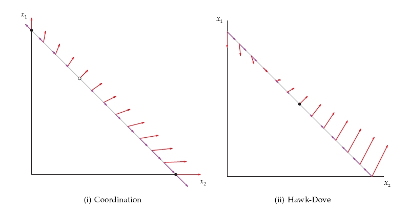
Figure 1. We show the dynamic of a population game. The red arrows indicate the direction that the frequencies of the strategies follow. The purple arrows indicate the projection of the red arrows onto a subspace of the strategies: in this case, the subspace is a line, corresponding to the points where the sum of frequencies is 1. The Hawk Dove Game is on the right. We show that in the Hawk Dove Game (but non in a simple Coordination Game) there is a stable point (The image comes courteously of Sandholm, Dokumaci & Lahkar, from SANDHOLM, W.H., Dokumaci, E., Lahkar, R. (2008) "The projection dynamic and the replicator dynamic", Games and Economic Behavior, 64-2:666-683). - 2.5
- We define π the average payoff for the whole population
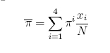
(2) - 2.6
- The replicator dynamic is
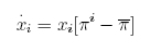
(3) i.e. under replicator dynamic, the frequency of a behavior increases when its payoffs exceed the average. For each time step t, the system of differential equations (3) defines a vector field (see figure 1). We call vector field a field that achieves the replicator dynamic F . We implement F by a global imitation algorithm. During the game, each agent tests whether another individual in the population has a greater payoff than its own. The main rule in this model is that an agent with a lower payoff imitates the behavior of another agent with a greater payoff. In our model, we don't have mutation in the imitation process. This theoretical framework directly derives from the formalization done by Ekman (2001).
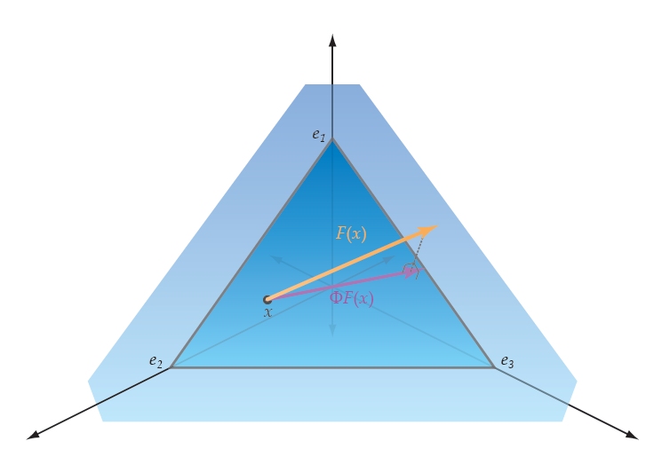
Figure 2. We show the projector dynamic of a population game with 3 strategies (The image comes courteously of Sandholm, Dokumaci & Lahkar, from SANDHOLM, W.H., Dokumaci, E., Lahkar, R. (2008) "The projection dynamic and the replicator dynamic", Games and Economic Behavior, 64-2:666-683).
The geometry of population games
-
Projector dynamic.
- 3.1
- The dynamic described by (3) is subject to a constraint since the number of agents remains constant, i.e. the sum of the xi must be 1. We could, thus, describe the dynamic of the game with a different approach, the so called Projector Dynamic (Sandholm et al. 2008). The key point of this approach is that the vector field F describing the population game is projected onto a new vector field
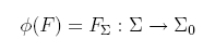
(4) where
(5) - 3.2
- Informally, we project the vector from F onto a line (if n =2), onto a bidimensional simplex (if n = 3, see figure 2) and so on. The projection of a vectorial field is a standard procedure. You can find an algorithm in Sandholm et al. (2008).
Projector dynamic with two strategies into RPSs game.
- 3.3
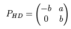
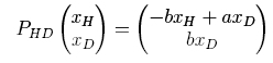
- We can explain the projector dynamic framework with two strategies using a 2-strategies RPSs game, the HawkDove game. In HawkDove game we fill the payoff matrix PHD (payoff matrix for a RPSs games) using the rules:
- when Hawk meets Dove Hawk win a;
- when Hawk meets Hawk both lose b with b < a;
- when Dove meet Dove both win b;
- when Dove meets Hawk, Dove gets 0.
(6) - 3.4
- If x is the vector of frequencies, we have
(7) hence from (7) we can compute the components of the projection of PHD for the HawkDove game
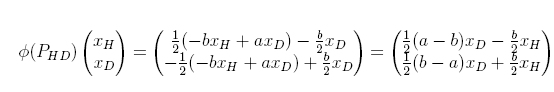
(8) The relation obtained for the projection let us state that the game has a stable stationary point (see figure 1, on the right)
Projector dynamic into congestion game.
- 3.5
- In the previous Subsection, we described the projector dynamic in RPSs Game, with constant 2-agents interactions payoff matrix. In our model (congestion game), we adapt the projector dynamic framework to compute a payoff matrix that starts from a payoff function with two parameters, i.e. the distribution of the strategies at time t and the combination of strategies at the same time.
- 3.6
- For example, we set a game where
- 2 hawks vis-à-vis 1 dove get a different payoff from the opposite situation (2 doves and 1 hawk)
- agents playing the same strategies interact (as in RPSs game Hawk-Hawk and Dove-Dove).
- 3.7
- We fill the payoff matrix PCG (payoff matrix for congestion game) using the following rules
- we fill the diagonal using the same strategy interactions, that is the interactions between the same strategies, for example Hawk-Hawk and Dove-Dove.
- we fill other cells using the different strategy interactions, that is the interaction between the corresponding strategy in a constant payoff matrix (in the simple case Hawk-Dove we consider the interaction between Hawk-Dove).
The model
-
The general framework: a junction
- 4.1
- Let P be a society consisting of a single population with N individuals. We consider a game where each individual follows one out of four behaviors, WatchRight, WatchLeft, Dove and Hawk. We denote the behavior with the index I. The frequency of individuals within the society with behavior i is xi.
- 4.2
- We define the behaviors and compute the payoffs because of the presence of 3 different algorithms: the conditioned, the compliant and the aggressive algorithm. The conditioned algorithm leads to WatchRight and WatchLeft behaviors. The compliant algorithm describes the Dove's behavior; the aggressive algorithm describes the Hawk's behavior. We use a discrete time model, following the scheduling in algorithm 1, where individuals are positioned randomly over a discrete bi-dimensional lattice L. We use a regular lattice, with C cell. We consider each cell of L a crossroad with four inputs (see figure 3).
- 4.3
- We describe the crossroads using counterclockwise direction and starting from West, if we are using a bird's-eye view. If we are using an individual view (i.e. the crossroad as it appears to the individual) we use the right, left and forward conventions (first we indicate what I find on my right, then on my left, finally in front of me). Hence, in Figure 3 (a) we show (1) an individual running East (with WatchLeft behavior); (2) the direction North-South is empty; (3) an individual with Hawk behavior is running to West; (4) an individual with Dove behavior is running to North. We call parallel the directions North-South and South-North, and the directions West-East and East-West. We define orthogonal the other combinations.
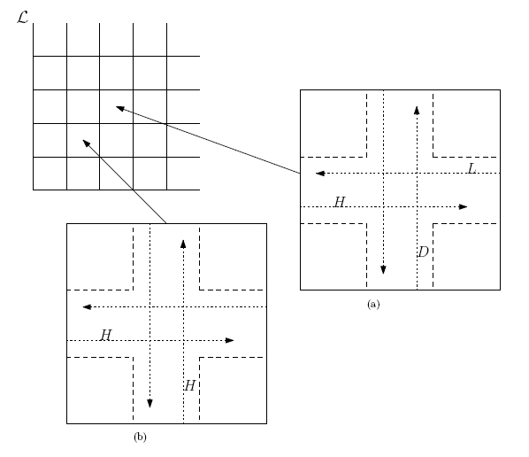
Figure 3. Two snapshots of L. In (a) we have 3 individuals, in (b) only 2; we put agents on the input of the junction, then they try to cross. There is no movement from a junction to another. - 4.4
- The model has some constraints:
- the individuals that are alone in a cell do not get payoff;
- a maximum of four individuals can occupy one single cell;
- only one individual per direction is admitted (it is not possible that, for example, two Hawks are running in the North-to-South direction);
- only orthogonal individuals (we mean individuals coming from orthogonal directions) matter.
Algorithm 1. The scheduling of simulation. We define as Crossroads the cells with more than 1 individual.
for t = 1 to T do
	for a = 1 to N do
		a := P
		to set a over L
	end for
	for c = 1 to Crossroads do
		Compute payoffs
	end for
for a = 1 to N do
		Imitation dynamic
	end for
end for
Algorithm 2. Conditioned. A is the individual. X indicates the direction to monitor. CRASH indicates that A goes into the crossroad at the same time of another orthogonal individual. STOP indicates that A does not go into crossroad. GOAHEAD indicates that the individual crosses the crossroad. H is a hawk individual. D is a Dove individual. C is a conditioned individual. We define not blocked C a conditioned individual with the free monitored direction.
If X is occupied then
	STOP
	else
		if there is (orthogonal H) or (orthogonal not blocked C) then
			CRASH
			else
				GOAHEAD
			end if
	end if
Algorithm 3. Aggressive.
if there is (orthogonal H) or (orthogonal not blocked C) then
	CRASH
	else
		GOAHEAD
	end if
Algorithm 4. Compliant.
if there is an orthogonal individual then
	STOP
	else
		GOAHEAD
	end if
Payoff computations
- 4.5
- To realize an analytic model for our congestion game, we write down an expression for πi, the payoff for i's strategy. More specifically, we have to write down a matrix PCG, 4 × 4. The elements of this matrix are functions of frequency of the strategies and the probability of the combinations of the strategies over the time. The computation of πi leads directly to fill the PCG matrix, using rules like in section 3.3, i.e. … we fill the diagonal using the same strategy interactions (for example WatchRight Vs WatchRight),… we fill the other cells using the different strategies' interactions (for example Hawk Vs Dove Vs WatchRight).
- 4.6
- We call the behaviors i, r =1, l =2, d =3, h = 4. The general rules are: if agent STOPS, the payoff is set to 0. If agents CRASH their payoffs are set to -1. If an agent GOESAHEAD, its payoff is 1.
- 4.7
- We let xi(t) denote the amount of individuals with behaviors i in period t. Clearly, we have x1 + x2 + x3 + x4 = N, where N is the total number of players. We also let C denote the total number of cells. We study the model with density C = N. The probability that one cell contains k individuals is
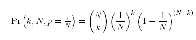
(9) - 4.8
- We call ak the number of cells with k individuals. We can compute the payoff for each behavior as the sum of the products between ak and the sum of the payoffs for each combination, with k fixed. For example for k = 2 we have 10 combinations, h = {rr, ll, dd, hh, rl, rd, rh, ld, lh, dh}. Only 8 combinations give some payoffs that are different from zero, rr, ll, dd, rd, rh, ld, lh, dh. hh does not give payoff, because we have parallel (=) hh with payoffs 2 and orthogonal (||) hh with payoffs -2. rl does not give payoff because for parallel combinations we obtain 2, and for the 2 orthogonal combinations (probabilities 1/2 and 1/2) we obtain 0 and -2.
- 4.9
- We call Khi the matrix of payoffs different from zero for behavior i and combination h. The probability of combination h with h1 + h2 + h3 + h4 = k conditioned to frequencies is a multinomial distribution
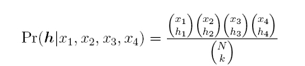
(10) - 4.10
- Finally, we can define the payoff for strategy i for strategy i
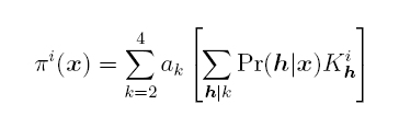
(11) 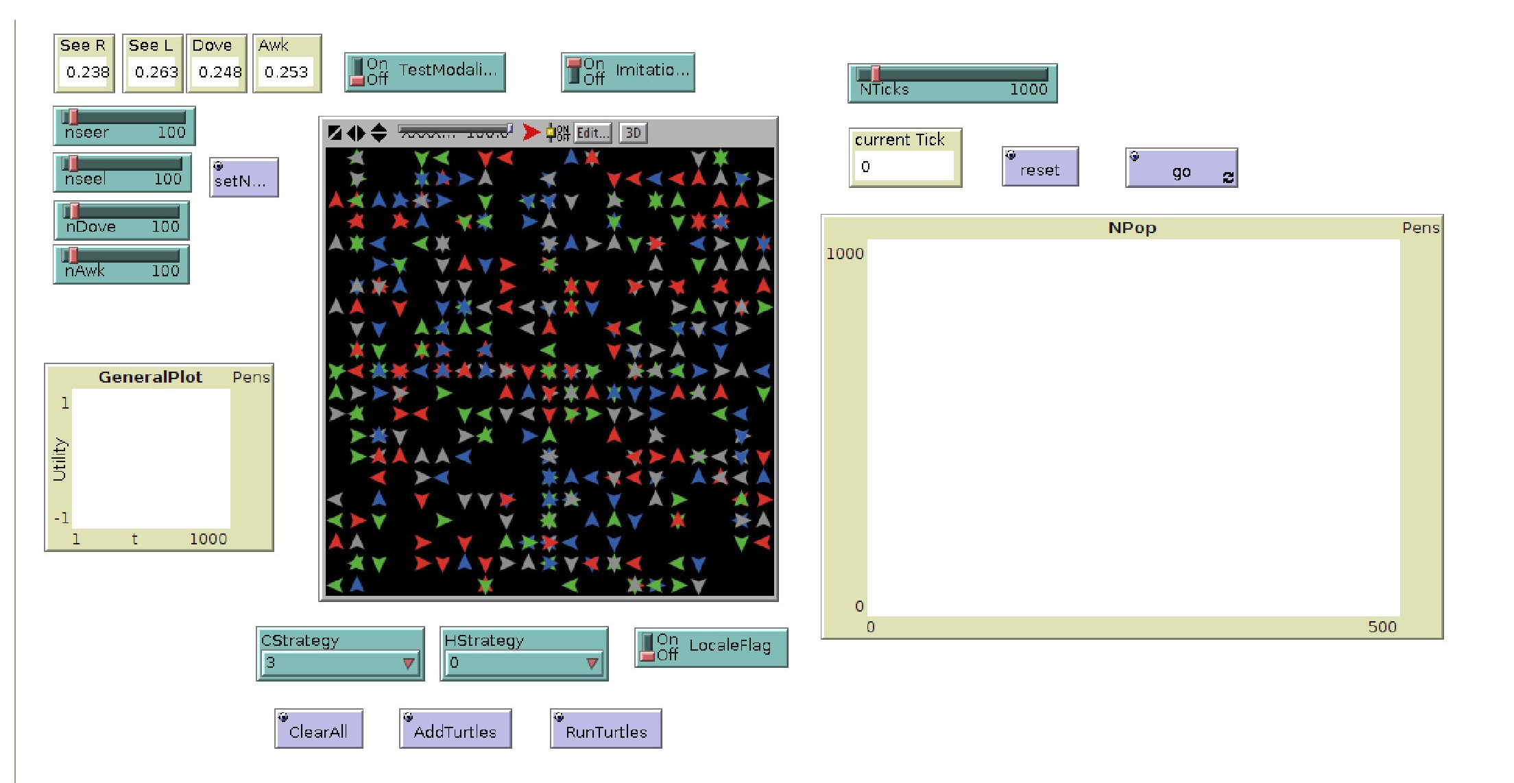
Figure 4. A snapshot of the simulator interface - 4.11
- Figure 4 is a snapshot of the simulator interface implemented in NetLogo.
In this interface each different strategy is represented by a different color:
- blue agents are right-watchers;
- gray agents are left-watchers;
- red agents are hawks;
- green agents are doves.
- 4.12
- Table 1 shows the parameters of the simulations.
Table 1: The set of parameters of simulations Parameter Value right-watchers from 50 to 200 left-watchers from 50 to 200 doves from 50 to 200 hawks from 50 to 200 # of Ticks 1000 Type of imitation global
Simulation results
- 5.1
- We run 256 simulations varying the size of each sub-population of agents between 50 and 200, thus the population's range varies from 200 to 800 agents. Each simulation includes 1000 ticks (see table 1 for the parameters). In figure 5, 6, and 7 we show some individual runs of the simulations.
- 5.2
- In accordance with the description above made of all of the possible steady states, we found the following results:
- one sub-population survives:
- Right-watchers: 3 times (1.18%);
- Left-watchers: 5 times (1.95%);
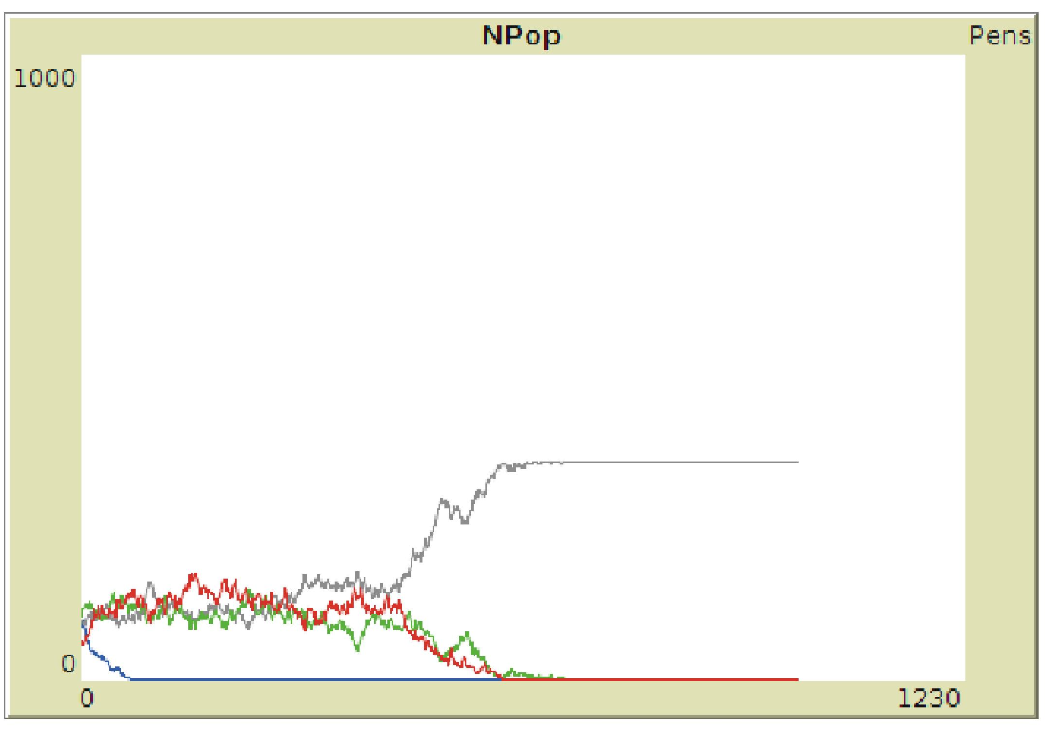
Figure 5. An individual run of the simulations. In this case, the simulation starts with 100 right-watchers, 100 left-watchers, 100 doves and 50 hawks and only left-watchers survive) - two sub-populations survive:
- hawks and doves: 48 times (18.75%);
- right-watchers and doves: 15 times (5.86%);
- left-watchers and doves: 19 times (7.42%);
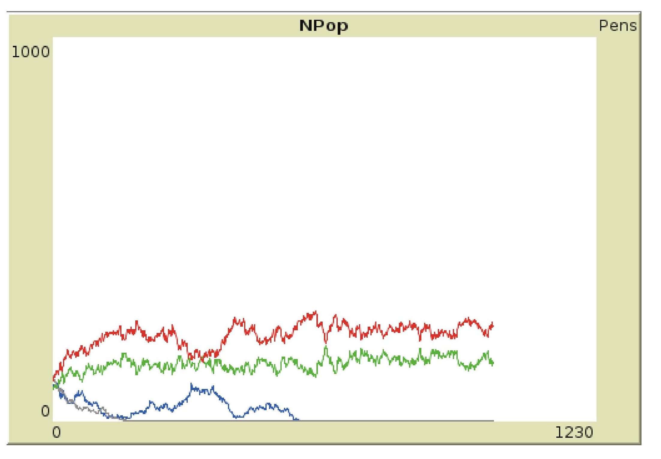
Figure 6. Another individual run. In this case, the simulation starts with 100 right-watchers, 100 left-watchers, 100 doves and 100 hawks and both doves and hawks survive) - three sub-populations survive:
- right-watchers and hawks and doves: 85 times (33.20%);
- left-watchers and hawks and doves: 81 times (31.64%);
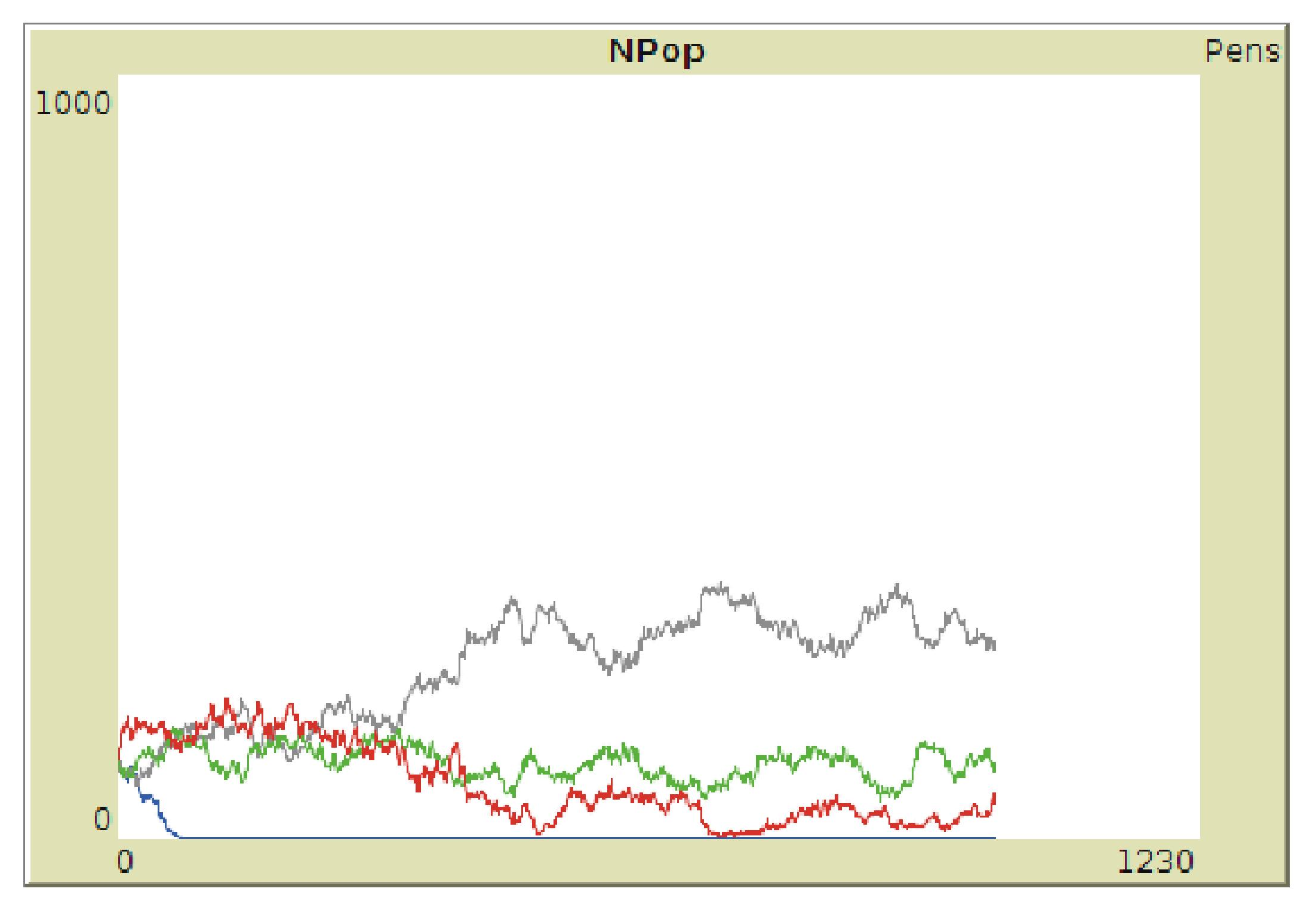
Figure 7. In this case, the simulation starts with 100 right-watchers, 100 left-watchers, 100 doves and 100 hawks and only right-watchers die
- one sub-population survives:
- 5.3
- Simulations may end up with multiple steady states (see figure 8; the tree shows the distribution of steady states. There are no outcomes that do not involve any sub-population : the number of agents remains constant):
- One sub-population survives: in this situation the sub-population can only be either right watching or left watching suggesting that, to put it in Lewis's terms, these are self-sufficient alternative solutions to problems of coordination. Being the two solutions equivalent, the choice between them is purely arbitrary. Thereby, once one solution has been selected, the other one cannot coexist.
- Two sub-populations survive. In this case,
- as it happens with the Evolutionarily stable strategy (ESS) (see Smith 1974; Gilbert 1981), if one sub-population is hawks, the other one will necessarily be doves; hawks do not survive with either right or left watching sub-populations;
- if, on the contrary, one of the sub-populations is doves, the other one may be any of the three remaining subpopulations, i.e. right watchers, left watchers or hawks.
- Indeed, unconditioned strategies are not symmetrical: the former can survive only by exploiting the most altruistic strategy.
- Three sub-populations survive by including either right watchers or left watchers sub-populations, but never both at once.
- Four sub-populations cannot survive (this is a consequence of the previous item).
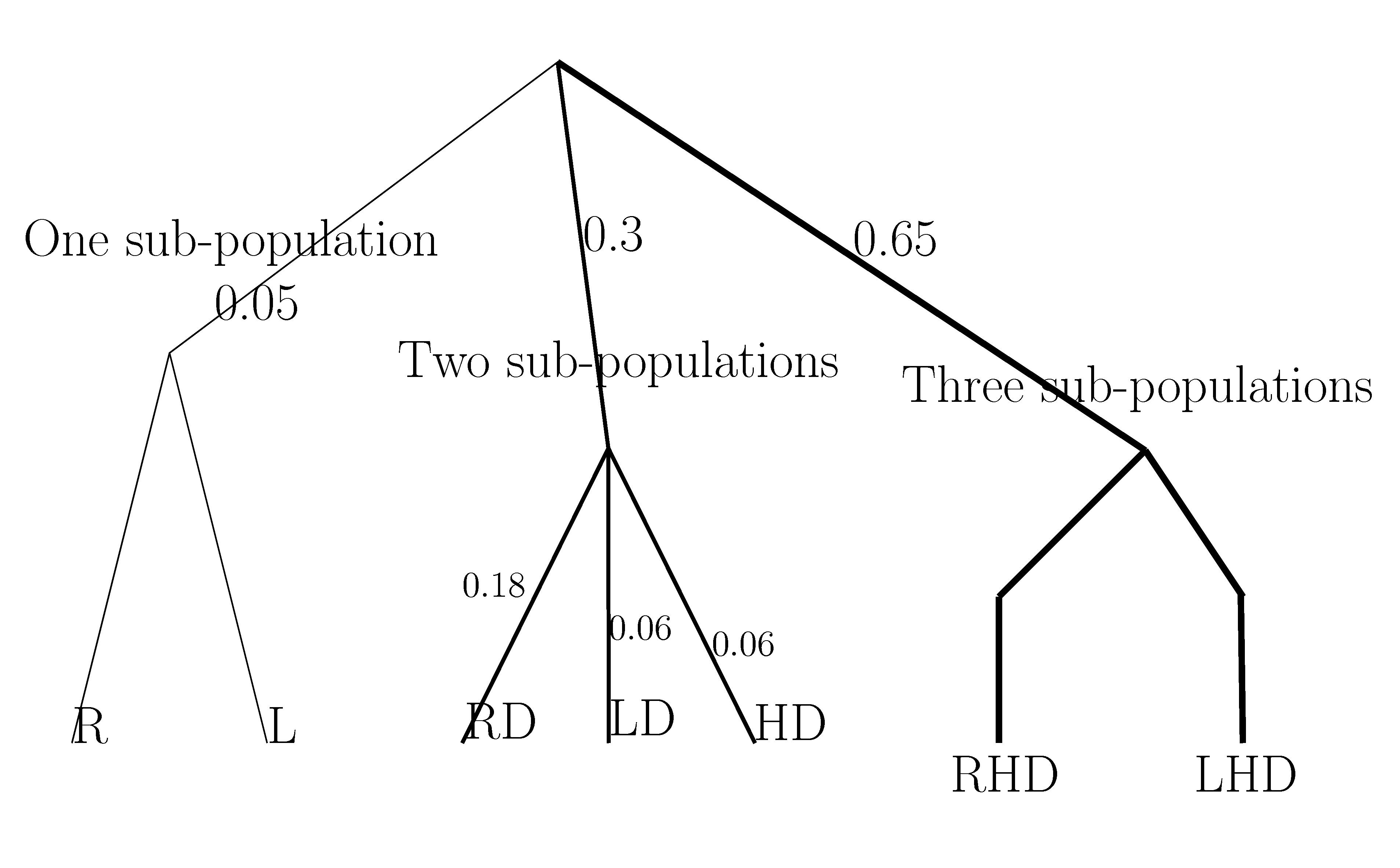
Figure 8. The tree shows the distribution of steady states. The width of the arrows indicate the frequency of the steady state (fat arrow means high frequency) - 5.4
- Summing all of the percentages, we can calculate all of the cases in which each sub-population (alone or with others) survives. We could define the adaptability of a sub-population the possibility of a sub-population to survive with another into a steady state. We can propose a hierarchy of adaptability:
- doves: 96.87%;
- hawks: 83.59%;
- right-watchers: 40.24%;
- left-watchers: 41.01%.
Analytic results
- 6.1
- We can extract information from the analytic model in three different ways. (1) we can numerically solve the differential equations system; (2) we can draw the vectorial field described by the ODE system; (3) finally, we can compute the steady states and the gradients around them, to valuate if the steady states are stable or not. Figure 9,10,11 show some examples.
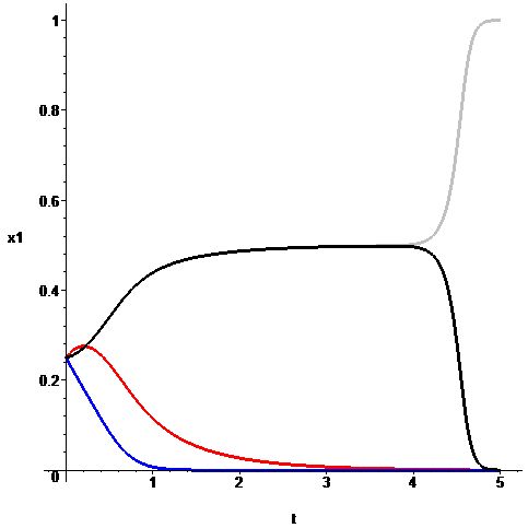
Figure 9. A numerical solution of the analytic model. The red curve shows the frequency of Hawks, the blue shows the frequency of Doves. The gray and the black curves show the frequencies of conventional strategies. 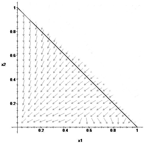
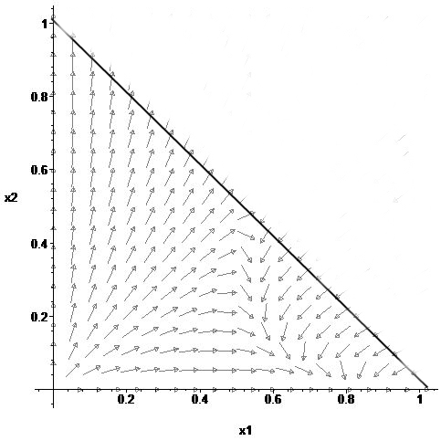
Figure 10. We show the direction of the vector field for the x1=right-watchers and x2=left-watchers. In the figure at the left, we set the number of hawks to zero. In the figure at the right, we set the number of doves to zero. We see that with no hawks, the steady state with two sub-populations is feasible 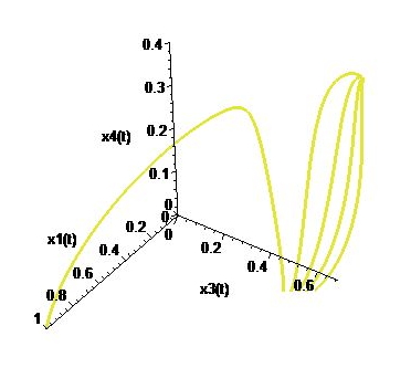
Figure 11. We have a map from the initial states with different numerousness to the steady states. In the figure we show that, starting with an average number of doves and a medium N, we have four paths on five to two-subpopulation steady states. (x1, x3, x4 means: right-watchers, doves and hawks. We set left-watchers to zero) - 6.2
- Using these methods, we obtained some analytic results, fitting with the simulation outcomes:
- The Conditioned strategy WatchRight and WatchLeft are incompatible. The relation obtained for the projection dynamic lets us state that the games with only one strategy have an unstable stationary point (the derivative of the frequencies has opposite sign, see figure 9). The initial state is almost uniform. We show that, after a delay, a conventional strategy wins (in this case the steady state is one-subpopulation): the dynamic show that the conventional strategies are incompatible.
- The Conditioned strategies on one hand and the Aggressive strategy on the other are incompatible. Vice versa, we find a stable steady state with Conditioned strategies combined with the Compliant strategy (see figure 10).
- 6.3
- The analytic model suggests some other hints:
- Figure 9 shows that we have a delay before separation between the Conditioned strategies. (the delay is observed during the simulation also). Thus, we could argue that the delay is not a stochastic effect coming from the fluctuations, during the agent-based simulation. The delay is the effect of the non-linearity of the interactions.
- By the EBM, we have a general map (the figure 11 is just an example) of the paths from the initial states, with different frequencies, to the final steady states. The map shows a correspondence with the steady states distribution from the simulations (0.05 one sub-population, 0.3 two sub-populations, 0.65 three sub-populations).
Discussion
- 7.1
- We try to summarize what might be the added value of this work (a) from the standpoint of understanding the role of conventions in congestion games (b) in the comparison between ABM and EBM approach in the study of social phenomena.
- 7.2
- Regarding section (a), in our ABM model we investigate the role of conditioned strategies - which can be seen as social conventions in Lewis's sense - in the solution of a congestion game, in comparison and in combination with unconditioned strategies.
- 7.3
- What do these results tell us about social conventions? In line with evolutionary game theory, this study helps to predict which strategies achieve a stable state. Besides, it allows new properties of strategies to be detected. In particular, we are able to discriminate not only between unconditioned and conditioned strategies, but also between incompatible equivalent strategies, i.e. strategies that have the same payoffs for all of the players, and complementary non-equivalent ones, i.e. strategies that benefit agents to a different degree (see the section on Simulation results). The former are self-sufficient, the latter are not. Hence, although we cannot predict which specific equilibrium will be achieved, we can tell the final composition of the population given a nth-strategy equilibrium.
- 7.4
- But is it true that we cannot predict which specific equilibrium will be achieved? Not completely. In fact, using EBM we can predict if a steady state should contain some combination of strategies, with which probability a steady state follows from some initial distribution, and the stability of steady states (see the results in the section on Analytic results).
- 7.5
- The point (b) is more controversial. The real question is: would it be possible to do ABM without EBM? And, on the other hand, would it be possible to realize the above-mentioned analytical model without the simulation data? Probably not. We claim that, for what concerns the social phenomenon we are interested in, i.e. the solution to a coordination problem in a large-scale population of heterogeneous agents in interaction, simulation data are decisive. The former already include features that are necessary for realizing the mathematical model. Nevertheless, we claim that these two classes of models are not alternative, but in some circumstances complementary. Let us try to defend this argument.
- 7.6
- The main difference between ABM and EBM is in the capacity to grasp different stochastic aspects of the phenomena. ABM describes stochastic fluctuations. EBM describes the statistics of the fluctuations, for example the mean, and the shape of the distribution.
- 7.7
- The results generated by the simulations may fit the analytical model: they provide in silico data for developing the analytical model to generalize the simulation results and to make predictions (Conte 2002; Bonabeau 2002).
- 7.8
- We also claim that neither the simulations nor the analytical model alone helped us explain why these data have been produced: in other words, none of the two methodologies helps us understand the data we have generated. Going back to our model, results show that playing with four qualitatively different populations, not only conventions emerge - i.e. equivalent arbitrary solutions to problems of coordination realized by the right watching or left watching populations - but also exploitation solutions, represented by the coexistence of "hawks" and "doves". In other words, dropping the 2-strategy game logics, hegemonic in Game Theory, it is by no means guaranteed that a conventional equilibrium will emerge.
- 7.9
- We can try some explanation, using the analytic payoff matrix. For example, the computation of payoff shows that there is a gradual deterioration of conditioned strategies proceeding from non-crowded to crowded world. In other words, if agents live in an environment where the likelihood of 4-agents junction is high, the advantage to maintain positive payoffs using conventional strategies disappears.
- 7.10
- Now, let us consider some facts emerging from the ABM framework. Suppose one sub-population survives: in this situation the sub-population can only be either "right watching" or "left watching", suggesting that, to put it in Lewis's terms, these are self-sufficient alternative solutions to problems of coordination. We show that these steady states occur rarely. Why? One possible answer (suggested by the EBM framework) could be that the number of paths from initial states to one sub-population steady state is low.
- 7.11
- Consider now the case in which two sub-populations survive: in this case, as it happens with Evolutionarily Stable Strategies (ESS), if one sub-population is "hawks", the other one will necessarily be "doves"; "hawks" will not survive with "right watching" or "left watching" sub-populations. These two latter results seem to suggest that unconditioned strategies are not symmetrical: although hawks and doves are not self-sufficient, the former can survive only by exploiting the most altruistic strategy. On the contrary, the latter is more adaptive, since it may survive in interaction with any other subpopulation.
- 7.12
- Hence, for a congestion game like the one discussed in this paper, we could try to define a hierarchy of adaptability. We find doves on the top: doves could live with hawks and conditioned agents; hawks could live with doves and, at the bottom, we find the conditioned agents. In fact, a conditioned strategy chases away the other conditioned ones. Hawks and doves are non-equivalent strategies: they have different payoffs, whose combination can be stable because of the complementariness of the two strategies.
- 7.13
- Three sub-populations survive by including either "right watchers" or "left watchers", but not both of them at once.
- 7.14
- At this point, one may come up with a rather obvious question: is it possible to predict, in general, the final states from the population size? The reader is reminded that we have analytically modeled all of the possible interactions in our scenario, and we have then calculated the point of equilibrium as a function of N, the dimension of the population (at least in theory). The analytic model allows the relationships between the strategies and their payoffs to be described through closed form equations and the simulation results to be generalized, allowing accurate predictions. However, this is an open point for discussion.
- 7.15
- Finally, a crucial feature concerns ABM: simulation results are organized in some hierarchical structure since they are generated by our algorithms. For example, in our model, the results incorporate peculiar symmetries: i.e. equivalent strategies cannot coexist, while non-equivalent ones can. We are attempting to explicate these results by EBM.
- 7.16
- The results generated by ABM simulations provide structured data for developing the analytical model through which generalizing the simulation results and make predictions. ABM simulations are artifacts that generate empirical data on the basis of the variables, properties, local rules and critical factors the modeler decides to implement into the model; in this way simulations allow generating controlled data, useful to test the theory and reduce the complexity, while EBM allows to close them, making thus possible to falsify them.
- 7.17
- In brief, Parunak , Savit and Riolo claimed that ABM and EBM differ in: i) relationships among the entities they model, ii) the level at which they operate. A look backward to the steps we followed to realize the analytical model provides us useful tips on the comparison between ABM and EBM. These two classes of models are not alternative, but in some circumstances complementary, and suggest some features distinguishing these two ways of modeling that go beyond the practical considerations provided by Parunak, Savit and Riolo.
Acknowledgements
- This work was supported by the EMIL project (IST-033841), funded by the Future and Emerging Technologies program of the European Commission, in the framework of the initiative "Simulating Emergent Properties in Complex Systems".
References
-
ARTHUR, W.B. (1994) "Inductive Reasoning and Bounded Rationality", American Economic Review , 84,406-411.
BONABEAU, E. (2002) "Agent-based modeling: Methods and techniques for simulating human systems", PNAS, vol. 99, pp. 7280-7287 [doi:10.1073/pnas.082080899]
CECCONI, F., Zappacosta, S. (2008) "Low correlations between dividends and returns: the alitalia's case", Proceedings of the IASTED International Conference on Modelling and Simulation (MS 2008), February, 13 - 16, Quebec, Canada
CECCONI, F., Zappacosta S., Marocco, D., Acerbi, A. (2007) "Social and individual learning in a microeconomic framework", Proceedings of the Econophysics Colloquium And Beyond, September 27-29, Ancona, Italia:
CHALLET, D., Zhang, Y.-C., (1997) "Emergence of cooperation and organization in an evolutionary game". Physica A 246, 407-418. [doi:10.1016/S0378-4371(97)00419-6]
CHALLET , D., Zhang, Y.-C., (1998) "On the minority game: Analytical and numerical studies". Physica A 256, 514-532. [doi:10.1016/S0378-4371(98)00260-X]
CHMURA, T., Pitz, T., (2006) "Successful Strategies in Repeated Minority Games". Physica A 363, 477-480. [doi:10.1016/j.physa.2005.12.053]
CHMURA, T., Pitz, T. (2007). "An Extended Reinforcement Algorithm for Estimation of Human Behaviour in Experimental Congestion Games", Journal of Artificial Societies and Social Simulation 10(2)1 https://www.jasss.org/10/2/1.html
CONTE, R. (2002) "Agent-based modeling for understanding social intelligence", PNAS, vol. 99, pp. 7189-7190 [doi:10.1073/pnas.072078999]
EKMAN, J. (2001) "Game theory evolving. a problem-centered introduction to modelling strategic interaction", Ecological Economics, 39(3):479-480 [doi:10.1016/S0921-8009(01)00247-6]
EPSTEIN, J. (2007) Generative Social Science:_Studies in Agent-Based Computational Modeling, Princeton University Press
GILBERT, M. (1981) "Game theory and convention", Synthese, 46:41-93 [doi:10.1007/BF01064466]
LEWIS, D.K. (1969) Convention: A Philosophical Study, Harvard University Press, Cambridge, MA
MILCHTAICH, I. (1996) "Congestion Games with Player-Specific Payoff Function", Games and Economic Behavior, 13, 111-124 [doi:10.1006/game.1996.0027]
ROSENTHAL, R.W. (1973). "A Class of Games Possessing Pure-Strategy Nash Equilibria", Int. J. Game Theory 2, 65-67. [doi:10.1007/BF01737559]
SANDHOLM, W.H., Dokumaci, E., Lahkar, R. (2008) "The projection dynamic and the replicator dynamic", Games and Economic Behavior, 64-2:666-683
SEN, S., Airiau, S. (2007) "Emergence of norms through social learning" in Proceedings of the Twentieth International Joint Conference on Artificial Intelligence(IJCAI'07), Hyderabad, India.
SMITH, J.M. (1974) "The theory of games and the evolution of animal conflicts", Journal of Theoretical Biology, 47:209-21 [doi:10.1016/0022-5193(74)90110-6]
SUGDEN, R. (2004) The Economics of Rights, Co-operation, and Welfare, Palgrave Macmillan, New York, NJ
PARUNAK, H.V.D., Savit, R., Riolo, R. (1998) "Agent-Based Modeling vs Equation-Based Modeling: A Case Study and Users' Guide", in Sichman, J., S., Conte, R., Gilbert, N. (eds.) Multi-Agent Systems and Agent-Based Simulation, Lecture Notes in Artificial Intelligence, pp. 10-25. [doi:10.1007/10692956_2]
YOUNG, H.P. (1993) "The evolution of conventions", Econometrica, 61:5784