
 Abstract
- This paper presents a model, using concepts from artificial neural networks, that explains how small rural communities make decisions that affect access to potable freshwater. Field observations indicate that social relationships as well as individual goals and perceptions of decision makers have a strong influence on decisions that are made by community councils. Our work identifies three types of agents, which we designate as alpha, beta, and gamma agents. We address how gamma agents affect decisions made by community councils in passing resolutions that benefit a village's collective access to clean freshwater. The model, which we call the Agent Types Model (ATM), demonstrates the effects of social interactions, corporate influence, and agent-specific factors that determine choices for agents. Data from two different villages in rural Alaska and several parameter sensitivity tests are applied to the model. Results demonstrate that minimizing the social significance and agent-specific factors affecting gamma agents' negative compliance increases the likelihood that communities adopt measures promoting potable freshwater access. The significance of this work demonstrates which types of communities are potentially more socially vulnerable or resilient to social-ecological change affecting water supplies.
- Keywords:
- Agent-Based Modeling, Artificial Neural Network, Social Network, Social Influence, Resilience, Freshwater
Introduction
- 1.1
- Communities in the Arctic of Alaska are increasingly faced with decisions that affect the supply and quality of critical resources such as water. Evaluating how effective social structures and institutions are in villages that make such decisions can determine which communities may best adapt under conditions of social (e.g., land use practices, population dynamics) and ecological (e.g., climate, permafrost, etc.) change. From available data, communities demonstrate significant variation in how their social network structures ultimately affect community-level decisions. In some villages, decisions that promote a community's resilience to social-ecological change can be made with relatively little difficultly, while in other villages such decisions are better described as wildcards, and in others still decisions leading to resilience are rare altogether.
- 1.2
- Artificial neural network and social network models have been developed by researchers in order to assess group dynamics and decision analysis (Garson 1998; Macy and Willer 2002; Newman and Park 2003). This methodology proves useful in determining how structured social networks can affect agent choices, ultimately influencing the evolution of the social system (Stocker et al. 2001; Shuguang and Chen 2008).
- 1.3
- This paper investigates example villages from rural Alaska
that have made decisions affecting access to potable freshwater
supplies. Our central research goal for this paper can be stated:
How do gamma agents affect decisions made by community councils in passing resolutions that benefit a village's collective access to clean freshwater?
Gamma agents, including alpha and beta agents, are individuals we identify as having important roles in community council decisions. The model we present could be a valuable analysis aid in assessing the effectiveness of local councils in addressing community freshwater needs. - 1.4
- In this paper, we present background information expounding village social structures and decision-making. A model using concepts from artificial neural networks that is applied within an agent-based modeling (Bonabeau 2002) approach is then presented. Two different village data sets are used for modeling, with details provided explaining specific model parameters. Model scenarios and outputs are discussed and, where relevant, compared to observed fieldwork observations. We present results from our parameter sensitivity tests to address relevant questions on model functionality and system-level change. A general discussion and future efforts to improve our work are then presented.
 Modeling
Background: Villages in Rural Alaska
Modeling
Background: Villages in Rural Alaska
- 2.1
- Village communities in many parts of rural Alaska are small and scattered, but are increasingly faced with a rapidly changing environment that is affecting freshwater supplies (Hinzman et al. 2005; Riordan et al. 2006). In addition to such change, increased land use activities, such as mining, have begun to affect water quantity and quality (Alessa et al. 2008). Under these circumstances, evaluating how communities respond to such change has become important in order to assess community resilience. One key indicator of effective response to change is the ability for communities to implement policies, such as building municipal water systems or installing filtration devices to improve water quality, that increase a community's resilience to freshwater change. Community responses are usually decided within village councils that determine whether or not to implement proposed resolutions.
- 2.2
- In the communities studied, three types of decision makers have been identified in fieldwork. These individuals act within community councils and represent the primary agents in our applied modeling approach. Our agent typology is similar to that used by Eguíluz et al. (2005), in which three agent types are defined similarly to our own. In addition, we recognize that Perez's (2009) work defines agents as selfish and principled (i.e., agents who care about norms), qualities that all three of our agent types integrate. Pérez's work borrows from Camerer (2003) and Fehr and Schmidt (2006) in defining how agents cooperate and motivations behind agent cooperation. In our case, rather than specifically focusing on cooperation, we are attempting to better understand how combinations of different types of agents, including the strengths of their social influence and relationships, can result in group decisions or consensuses being made. This form of analysis seeks to understand the underlying critical social mass of agent types and their attributes that are necessary to enable collective action to take place, similar to what is demonstrated by Marwell and Oliver (1993). The types of agents used here can be referenced as alpha (α), beta (β), and gamma (γ) agents, a designation that has been developed elsewhere (Alessa and Kliskey 2010).
- 2.3
- Alpha agents are considered the initiators in the community; these individuals not only initiate ideas, but also sustain efforts in order to promote freshwater resilience. These agents develop ideas based on perceived needs, work with other α-agents, and attempt to convince others that their ideas can benefit the community. In a changing Arctic, we see these individuals as critical resources for communities since they are better able to perceive change that is occurring and organize an adequate response to that change. Beta agents differ in that they are not usually the individuals who instigate community response promoting resilience, but generally have goals that are community focused. Gamma agents, like α-agents, often have high initiative. However, they differ in one fundamental characteristic: these agents primarily have self-serving goals rather than goals aimed at corporate benefit. Gamma agents can be swayed to go along with community resolutions, but generally need to perceive self-benefit in the decision made. Gamma agents can disrupt initiatives promoted by α-agents if initiatives are counter to their individual goals. In reality, agents display some qualities from each of the other agent types; the categories we present, therefore, are a continuum of values that describe agent goals and behaviors. Values governing agent goals and behaviors each concentrate near three specific discrete points in a continuum.
- 2.4
- Members in the community decision body generally deliberate and decide after a period of time from when the proposed measure is presented. Resolutions that pass are then implemented, with some of
- 3.2
- these decisions requiring sustained management and further resolutions if built infrastructure (e.g., building and maintaining a municipal water system) is involved. In certain cases, councils may be effective in reaching a consensus to implement a resolution promoting freshwater access; however, council members may prove to be unable to sustain commitment to that choice. An example of inadequately sustained decisions is a lack of supervision or provision of funds that enable the long-term maintenance of freshwater infrastructure.
Applied
Modeling Approach
- 3.1
- The simulation we built is written in Java and has been applied within Repast Simphony (Repast 2009). The simulation itself can be downloaded, with instructions provided in the model folder.
- 3.2
- To address issues on decision-making affecting access to potable freshwater resources, researchers have implemented modeling approaches that use agent-based methodologies incorporating group behavior and learning (Pahl-Wostl 2002). In our agent-based approach, we use concepts from attractor artificial neural networks developed by Hopfield (1982), with functionality most similar to a model developed by Kitts (2006). We feel this approach is appropriate because it accounts for relationships and influence between individuals, individual factors that affect decision-making, and feedback effects that influence future agent interactions and decisions. In our approach, agents are treated as nodes in a network, with each agent tracking satisfaction with a choice made. Nodes are connected by links made up of two values, including weights that describe the strengths of relationships and binary values showing approval/disapproval of other agents in network links.
- 3.3
- In our applied model, which we call the Agent Types Model (ATM), weights in links evolve based on a learning rule that evaluates previous states of the network structure using Hebbian learning (Hebb 1949). A community object is created and implements ATM, with each person agent (i.e., α-, β-, and γ-agents) in the community evaluating social relationships with all other agents. Social weights and approval within the network links are continually adjusted, with agents determining their choice to agree or disagree with the community-level proposition in each simulated round. Having some similar aspects to Pujol et al. (2005) and Stocker et al. (2002), agents make decisions, to disapprove/approve of other agents and accept/reject a choice, through bounded rationalized choices that are based on local knowledge and understanding of other agents, including those agents' overall social influence. Conceptually, agents make decisions based on their experience with localized interactions with other agents as well as individual perceptions and goals relative to a given choice, similar to individual behavior within networks as described by Holland (1998).
- 3.4
- Figure 1 shows an example network of three agents. In this
network, agents have parameter states that define if they are compliant
or not with a given choice option, weights between agents ranging from
-1 to 1, and links showing if agents approve or disapprove of their
social connections. In essence, ATM attempts to balance variables
relative to each other in order to reach a more stable network state.
Appendix A provides a detailed
explanation of ATM's steps.
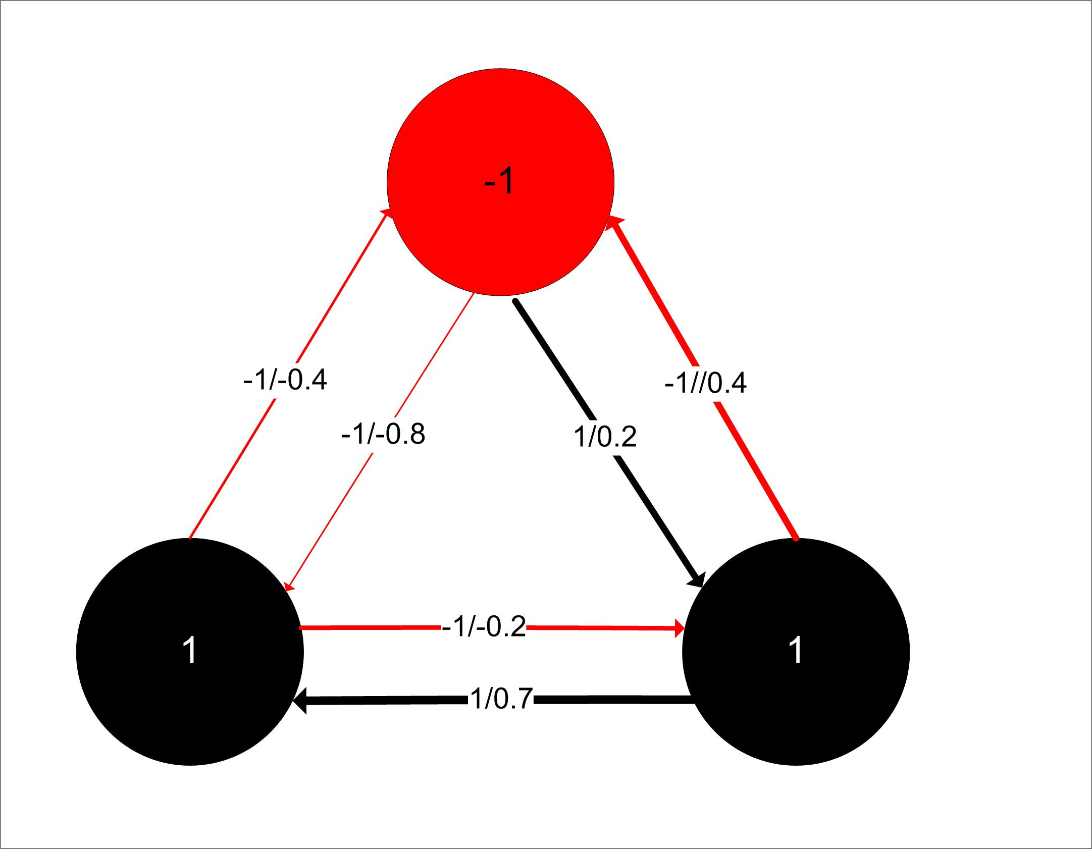
Figure 1. Image indicating an example network of three agents. Links between the agents (circular objects) show disapproval/approval (-1 or 1) and weight values (-1 to 1) that define social relationships. Red edges indicated disapproval by an agent (-1), black edges indicate approval (1), and line thickness depicts relative weight values (i.e., thin is a weak weight, thick is a strong weight). Agents who reject (-1) a choice are indicated as red; black agents are those who accept (1) a choice. Model Data and Parameterization
- 3.5
- Data characterizing two villages in rural Alaska are used in modeling scenarios. We present the scenario data in Tables 1-2. Parameterization is based on quantitative valuations using qualitative field observations. Since we could not obtain quantitative values from subjects, data are derived from fieldwork observations of individual behaviors during a one-month period. The observations include interactions between individuals, importance of individuals in social interactions, social cost for accepting decisions, how individuals learn (i.e., collective- vs. individual-based learning), and goals of individuals (i.e., collective vs. individual goals). Qualitative observations were assigned numeric values and are reflected in the discussion provided below.
- 3.6
- The agent-specific variables used are as follows:
- Type=Agent type (i.e., α, β, or γ)
- WeightA = Link weight distribution of agents to α-agents, with values provided used in a beta distribution as the alpha and beta inputs (e.g., 6/4, α=6, β=4). Weight distributions reflect social influence of α-agents.
- WeightB = Link weight distribution of agents to β-agents, with values provided used in a beta distribution as the alpha and beta inputs. Weight distributions reflect social influence of β-agents.
- WeightC = Link weight distribution of agents to γ-agents, with values provided used in a beta distribution as the alpha and beta inputs. Weight distributions reflect social influence of γ-agents.
- Importance = Relative importance of an agent in community decisions, with values ranging from 0 to 1 (0 is the low importance, 1 is high importance)
- DecisionCost = The cost variable for an agent to make a decision, with values ranging from 0 to 1 (0 is low cost, 1 is high cost).
- 3.7
- Similar to other simulation parameterization, we obtain initial weight values for network links from beta distributions using the alpha and beta inputs outlined above (Fleischmann 2005). Rather than the standard 0 to 1 beta distribution, our distribution scales the outputs to reflect values from -1 to 1. As is similar to other efforts applying qualitative data to agent-based modeling, we attempt to make weight distributions varied enough to reflect representation that are similar to our qualitative observations of individuals. We also test the sensitivity of weight values in order to observe how much change is needed before significantly different, both qualitatively and quantitatively, results occur (Yang and Gilbert 2008). Values presented, therefore, reflect ranges that have been tested for their relative qualitative representation (e.g., low weight value interpreted as "negative" social influence by agents) and influence on changing model results. In fact, this is true for all relevant parameters presented, even those inputs not used in any random distribution. Parameter sweeping and sensitivity testing, unit testing, code walkthroughs, debugging, and visual and statistical analysis of outputs were used for verification of modeling procedures (North and Macal 2007).
- 3.8
- In general, α-agents can be described as having positive
connections with each other, but social consideration received from
β-agents is weaker, while social connections are generally negative
with γ-agents. Beta agents, on the other hand, are usually positively
connected to α-agents in that their social inputs are valued, while
weights are more evenly distributed among the other agent types. Gamma
agents often have positive relationships with each other, but their
connections are generally negative with α-agents and either positive or
negative with β-agents. In most cases, α-agents have high importance
values, but in some cases the importance of α-agents is relatively weak
or γ-agents can be relatively influential. For decision costs, γ-agents
often perceive water projects as more costly, as they may require some
personal financial or other sacrifices, while other agents often do not
see such projects as a major cost.
Table 1: Input values for the first village scenario Type WeightA WeightB WeightC Importance DecisionCost beta 8/2 5/5 5/5 0.1 0.1 beta 8/2 5/5 5/5 0.1 0.1 beta 8/2 5/5 5/5 0.1 0.1 beta 8/2 5/5 5/5 0.1 0.1 gamma 3/7 5/5 8/2 0.5 0.5 gamma 3/7 5/5 8/2 0.5 0.5 gamma 3/7 5/5 8/2 0.5 0.5 gamma 3/7 5/5 8/2 0.5 0.5 beta 8/2 5/5 5/5 0.1 0.1 beta 8/2 5/5 5/5 0.1 0.1 beta 8/2 5/5 5/5 0.1 0.1 beta 8/2 5/5 5/5 0.1 0.1 alpha 8/2 5/5 2/8 0.5 0.1 alpha 8/2 5/5 2/8 0.5 0.1 alpha 8/2 5/5 2/8 0.5 0.1 Table 2 Input values used for the second village scenario Type WeightA WeightB WeightC Importance DecisionCost beta 8/2 5/5 5/5 0.1 0.1 beta 8/2 5/5 5/5 0.1 0.1 beta 8/2 5/5 5/5 0.1 0.1 beta 8/2 5/5 5/5 0.1 0.1 gamma 2/8 5/5 8/2 0.8 0.6 gamma 2/8 5/5 8/2 0.8 0.6 gamma 2/8 5/5 8/2 0.8 0.6 beta 8/2 5/5 5/5 0.1 0.1 beta 8/2 5/5 5/5 0.1 0.1 beta 8/2 5/5 5/5 0.1 0.1 beta 8/2 5/5 5/5 0.1 0.1 beta 8/2 5/5 5/5 0.1 0.1 alpha 8/2 5/5 2/8 0.5 0.1 alpha 8/2 5/5 2/8 0.5 0.1 alpha 8/2 5/5 2/8 0.5 0.1 - 3.9
- These two tables (Tables 1-2) represent scenarios in which villages have been somewhat able and unable to pass resolutions respectively affecting access to potable freshwater. We did not model cases in which villages were almost always successful in addressing potable freshwater needs because our examples in those cases produced results that were exceedingly obvious. In those cases, few γ-agents were apparent.
- 3.10
- Two other variables are applied and not indicated in the
tables. These are affective dependence (D; measures
if an agent values collective good vs. individual approval) and
normative dependence (δ; agent decisions made based on individual
learning or social learning). Similar to the weight inputs, these two
variables are determined by a beta distribution (e.g., 8/2, α=8, β=2)
that randomly parameterizes the values, although these variables are
not scaled. For all scenarios, unless otherwise stated, α-, β-, and
γ-agents have affective and normative dependence variables defined by
the inputs in Table 3. In effect, these variables help to distinguish
differences between agent types.
Table 3: Values used for parameterization of a beta distribution that determines affective and normative dependence inputs for agent types Variable Type α β γ Normative Dependence (δ) 8/2 8/2 2/8 Affective Dependence (D) 2/8 2/8 8/2 - 3.11
- In addition to these data, the approval parameters (-1 or 1 for disapprove and approve respectively) in social links are initialized deterministically for link weight values that are less than -0.1 and greater than 0.1. Weight values between -0.1 and 0.1, since they are relatively near neutral (i.e., 0) and may result in either negative or positive approval, produce approval states that are determined via the probability function defined in Appendix A (13). The initial noncompliance or compliance (i.e., c=-1 or 1 respectively) decision for β-agents is set randomly based on a 50% probability. Alpha agents are always set to accept a decision, while γ-agents accept a decision based on the probability that a random value from a uniform distribution (0 to 1) is greater than a γ-agent's individual cost value (e).
Simulation
Results
- 4.1
- In addition to two scenarios depicting observed villages,
we present parameter sensitivity studies that highlight model
functionality and the effect parameter changes in γ-agents have on
overall system-level compliance. We focus on the compliance output as
this directly relates to the central question asked in the
introduction. Other variable outputs were evaluated in the course of
model verification; these can be evaluated in ATM. Each scenario was
executed 1000 times, enough runs to account for stochastic variation
and demonstrate model trends, with results reflecting the output
aggregations for all runs in a scenario. In general, compliance varies
more greatly early in simulations, but later the results are narrower
as ATM begins to reach a more balanced state. Each tick, therefore, has
a compliance result that is based on averaging compliance for all of
the simulation runs. Appendix B
presents summary statistics for different scenarios, indicating the
mean and standard deviation for compliance response by the modeled
group. In addition to these statistics, compliance distributions in
scenarios were compared to each other using a Wilcoxon signed-rank test
to indicate levels of statistical significance. All statistical tests
were conducted within R (R Project 2009).
Scenario 1
- 4.2
- In this scenario we applied data from Table 1, which represent data from a small village that has more γ-agents than α-agents. The exact number of agents involved in the decision process is higher; agents in each category were downscaled to reflect ¾ the size of the actual number of decision makers. Since we are primarily interested in the ratio of agent types involved in decision processes, and our data are not yet detailed enough to allow clear differentiation of all the agents involved in the decision process, ATM is equally functional with only ¾ of the total agents involved. In other words, we tested this scenario with 100% representation of agents, but it produced virtually the same results as this ¾ size case. In addition, sociometric visualization proved to be easier to comprehend with fewer agents. Supplementary to the summary statistics provided in Appendix B, average agent weights at specific time steps can be plotted in two-dimensional graphs using the PCA function described earlier. The results highlight the number of agents who agree to the choice as well as the sociometric location of agents to each other over the modeled time steps (Figures 2-6).
- 4.3
- At the beginning of the scenario (i.e., Figure 2), agents
are split into three groups comprising of α- (agents 12-14), β- (agents
0-3 and 8-11), and γ-agents (agents 4-7). Early in the simulation, most
agents are generally compliant with the choice option (Figure 3). After
these initial ticks, β-agents begin to show an average compliance
choice ranging between -0.01 and 0.01, indicating either a slightly
negative or positive compliance average (Figure 4). In the case shown,
compliance was slightly positive for all β-agents, indicating overall
weak compliance. At Tick 400, agents become generally more noncompliant
(Figure 5). In fact, agents 0-3 and 8-11 become slightly more socially
affiliated with the γ-agents (agents 4-7). By the end of the scenario,
agents are once again bordering mild compliance or noncompliance,
although in most cases the agents are usually slightly negative in
their compliance (Figure 6). The sociometric visualization indicates
that the β-agents are more closely linked to the γ-agents. Average
compliance results for the entire simulation indicate that compliance
generally fluctuated near zero for most of the simulation (Figure 7).
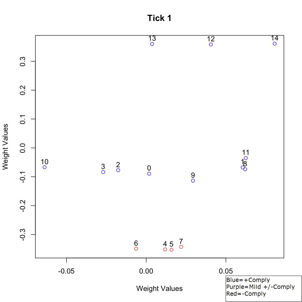
Figure 2. Sociometric space at Tick 1 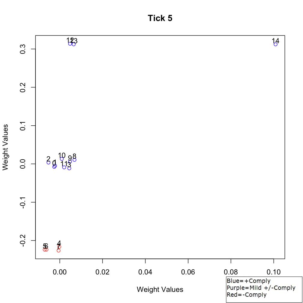
Figure 3. Sociometric space at Tick 5 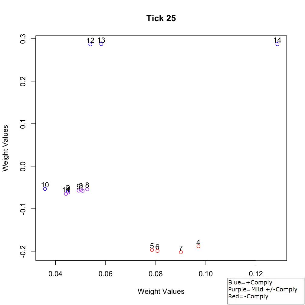
Figure 4. Sociometric space at Tick 25 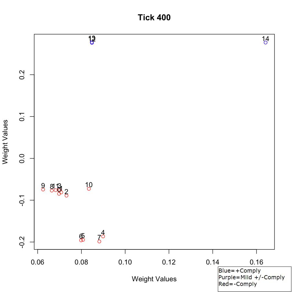
Figure 5. Sociometric space at Tick 400 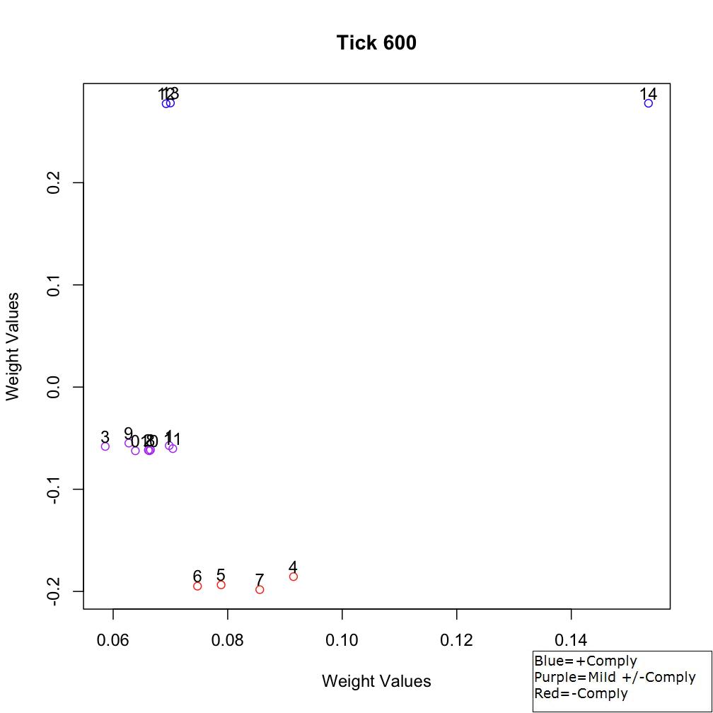
Figure 6. Sociometric space at Tick 600 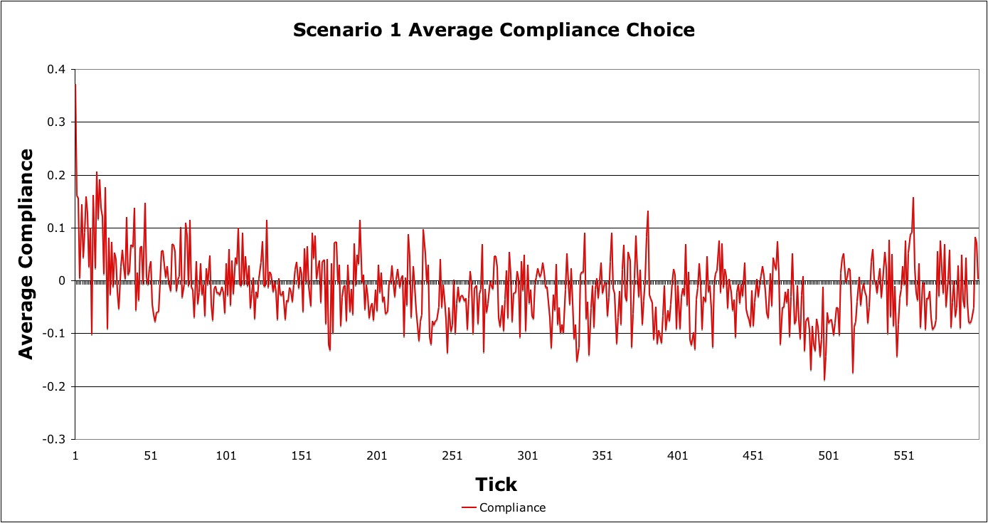
Figure 7. Average compliance response in Scenario 1 - 4.4
- Qualitative field observations can be compared to modeling
results to indicate if the simulation results could be expected. Data
collection teams working in this village have observed that
propositions affecting water quantity/quality have, in fact, been
passed. In one example, a water filtration facility was voted on, with
the resolution passing. However, in this case, there have been a number
of delays in the construction and instillation of the facility, with
the council being generally ineffective in enforcing its decision. In
fact, the γ-agents involved were successful in stalling enforcement of
the measure, as these agents controlled the construction team that
would have been needed to install the water system. What this suggests
is that the village council is weak, similar to the weak positive or
negative compliance values obtained from ATM. Certainly, this is not a
strong validation of ATM, but it provides an initial indication if the
model is potentially applicable for this village's decision scenarios.
Scenario 2
- 4.5
- Table 2 was applied in this scenario, with the number of
agents downscaled to ½ of the actual number of individuals for the same
reasons as Scenario 1. As seen in the previous scenario, α- (agents
12-14), β- (agents 0-3 and 7-11), and γ-agents (agents 4-6) are
initially separated in sociometric space (Figure 8). In the first few
ticks, agents seem to be positive or slightly positive or negative in
their compliance responses (Figure 9). Soon, however, agents have a
strong tendency for noncompliance and generally remain at this state
for the duration of the simulation (Figure 10-11). Comparing the
results to the last scenario (Figure 11 vs. Figure 6), β-agents are
more clearly associated with γ-agents. In addition, Appendix B indicates that the p-value obtained
by comparing the two compliance distributions for Scenarios 1 and 2
shows significant differences. The overall results indicate relatively
strong negative compliance by the community council (Figure 12).
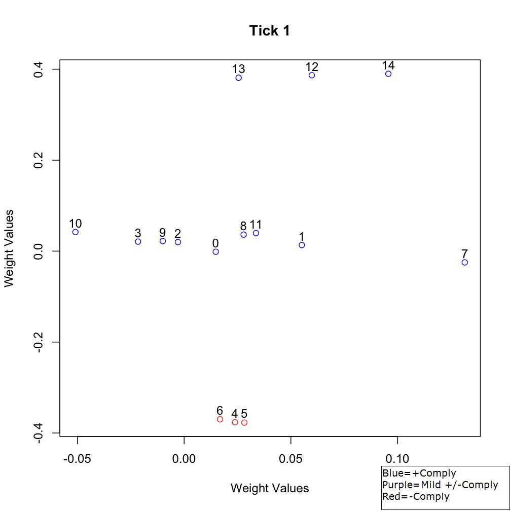
Figure 8. Sociometric space at Tick 1 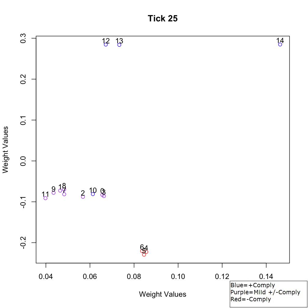
Figure 9. Sociometric space at Tick 25 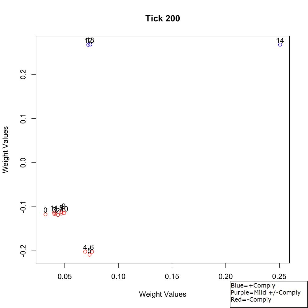
Figure 10. Sociometric space at Tick 200 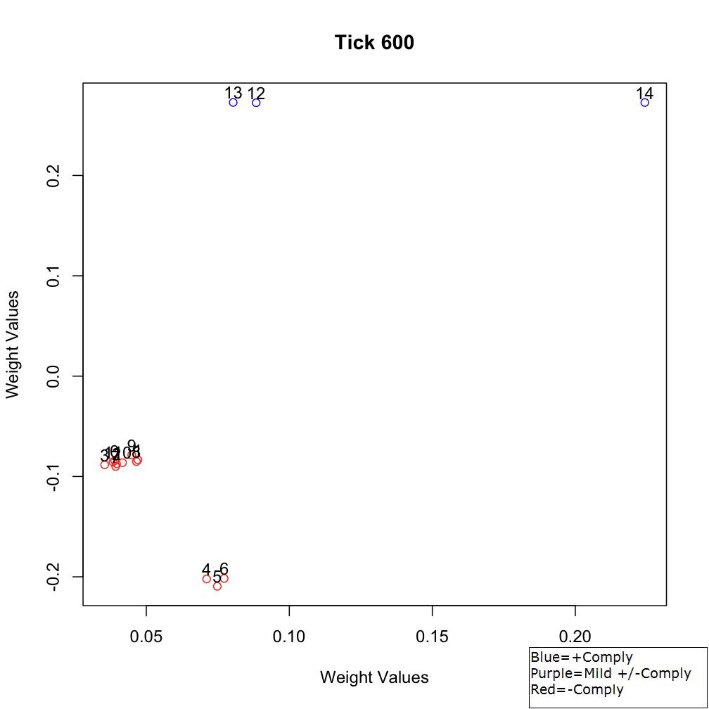
Figure 11. Sociometric space at Tick 600 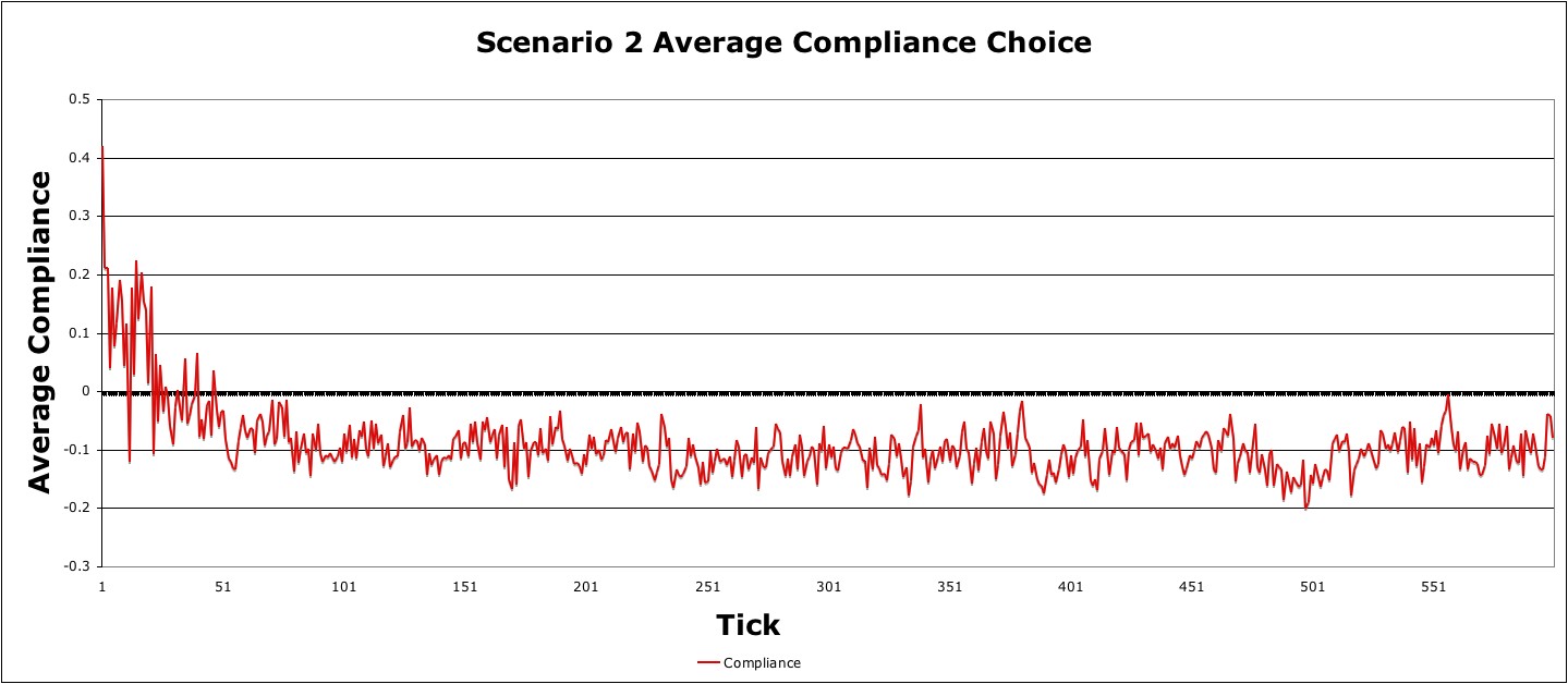
Figure 12. Average compliance during the duration of the simulation - 4.6
- As for comparing simulation results with field
observations, again some qualitative assessment can be made. This
village was observed to be unable to pass any resolutions that may
benefit water delivery or quality for residents. In fact, recent
observations indicate that the decision council was generally
unorganized and incapable in uniting the decision brokers to come up
with a necessary consensus for addressing community water needs.
Scenario 3a-d
- 4.7
- In order to better observe how ATM performs, certify that
the model functions according to our stated goals, and understand how
changes in a specific variable could affect the social system, we
performed a series of sensitivity tests to applied parameters in
γ-agents (North and Macal 2007;
Midgley et al. 2007).
Here, we attempt to investigate at which level of importance do
γ-agents need to be reduced to in order to have significantly less
negative influence on β-agent compliance. In this case, we change the
importance input for γ-agents to values that range between 0.4 and 0.7,
with all other variables using values from Scenario 2. As summarized by
the results in Appendix B, the
sub-scenarios (a-d) show that there are statistically significant
differences between this scenario (Scenario 3a) and Scenario 2 and
within the different parameter settings for this scenario (Scenario
3b-3d). Based on qualitative observation, the results suggest that the
reduction of the importance parameter to 0.4 or less lead to compliance
being generally positive (i.e., compliance averaging above 0.1), while
values at 0.5 or greater make the community slightly positive or
negative in compliance. Visually, however, output results between 0.4
and 0.6 are not very different (Figure 13).
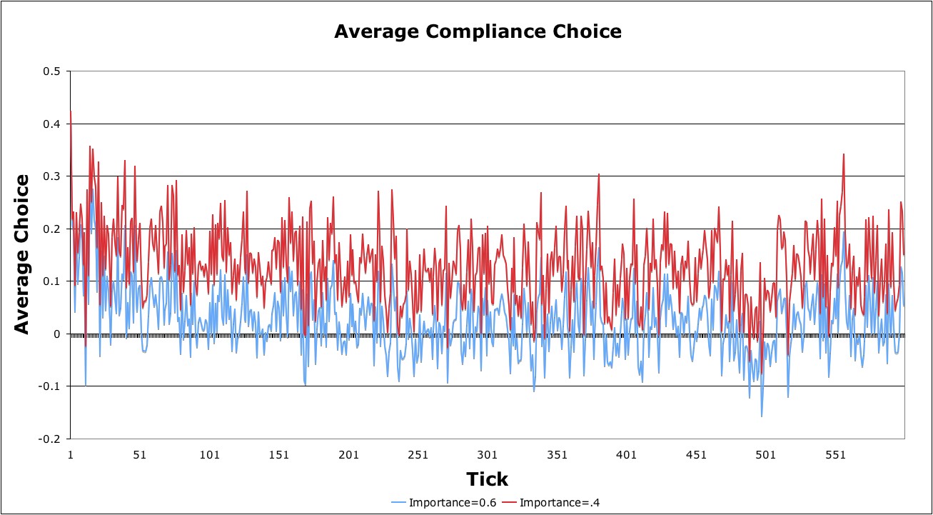
Figure 13. Two of the importance parameter settings (0.4 and 0.6) are tested for their effect on compliance choice Scenario 4a-d
- 4.8
- In addition to testing sensitivity to the importance
parameter, we tested changes to the decision cost parameter. The
question we had in this scenario was to what extent can changes in
decision cost cause γ-agents to comply with a proposition? We used the
same parameters as Scenario 2, with the exception of the decision cost
parameter changed for the γ-agents (Appendix B).
In general, ATM proved to be more sensitive to changes in this
parameter, as changes of 1/10th caused qualitatively different results
to compliance. As an example, decision cost values at 0.4 for γ-agents
result in the overall compliance being significantly positive, while at
0.5 the results were not significantly positive (Scenarios 4a and 4b;
Figure 14). Even at the 0.4 level, however, γ-agents were still
somewhat negative in their compliance. Decision cost values at 0.2
(Scenario 4d), on the other hand, did make γ-agents more positive in
compliance, as apparent in Tick 600 (Figure 15). In fact, for the 0.2
decision cost value, the sociometric visualization at Tick 600 shows
that all agents, including γ-agents, were clustered far closer together
than in other scenarios, showing greater social cohesion for the group
as a whole. This relative cohesion remained generally consistent until
the end of the simulation. Comparisons of distributions between this
scenario (Scenario 4a) and Scenario 2 and within this scenario
(Scenario 4b-4d) showed statistically significant distribution changes.
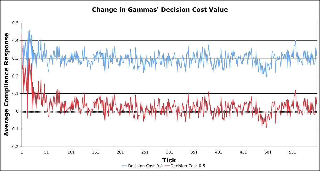
Figure 14. Scenario measuring the effect of decision cost change on average compliance response 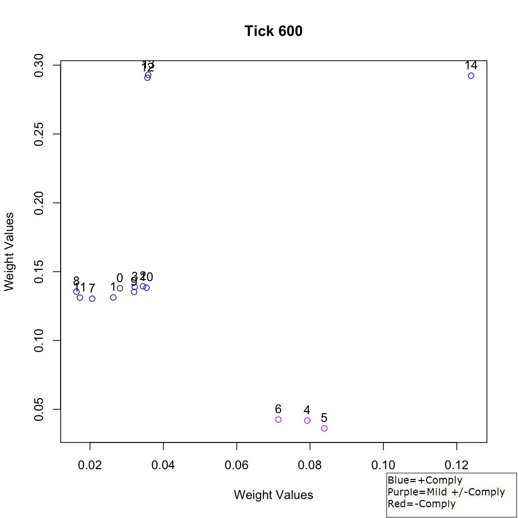
Figure 15. Sociometric space at Tick 600 with the decision cost parameter set to 0.2 for γ-agents Scenario 5a-d
- 4.9
- In this scenario, we test normative dependence by a
sensitivity analysis on γ-agents. The question this scenario attempts
to address is how much does normative dependence have to change for
γ-agents before significant system-level changes can be observed?
Similar to the previous cases, we use the initial inputs from Scenario
2 (Appendix B). In general,
very minor qualitative changes (i.e., compliance choices becoming
strongly positive) occur between this scenario and Scenario 2 until we
tested normative dependence at α/β ratios, used for the beta
distribution discussed for this parameter, greater than 6/4 (i.e.,
Scenario 5b-d). In fact, looking at sociometric visualizations of Tick
400 for the 6/4 and 7/3 ratios, very different results between these
ratios are apparent (Figures 16-17). The 6/4 ratio results in most of
the agents having negative compliance, while the 7/3 ratio produces a
strong positive compliance. In addition, in the 6/4 ratio case
(Scenario 5a), the compliance result between Scenario 2 and this
scenario is not significantly different (i.e., p-value < 0.01),
while at the 7/3 level β- and γ-agents are clustered closely to each
other and there is overall positive compliance. Looking at the overall
compliance averages for normative dependence ratios at 6/4, 7/3, and
8/2, the dramatic differences in results are self-evident (Figure 18).
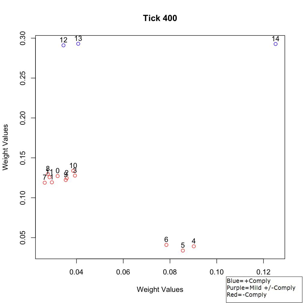
Figure 16. Sociometric space at Tick 400 with the normative dependence parameter set to 6/4 in γ-agents 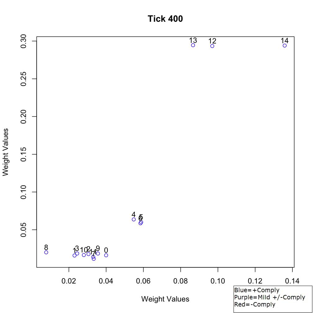
Figure 17. Sociometric space at Tick 400 with the normative dependence parameter set to 7/3 in γ-agents 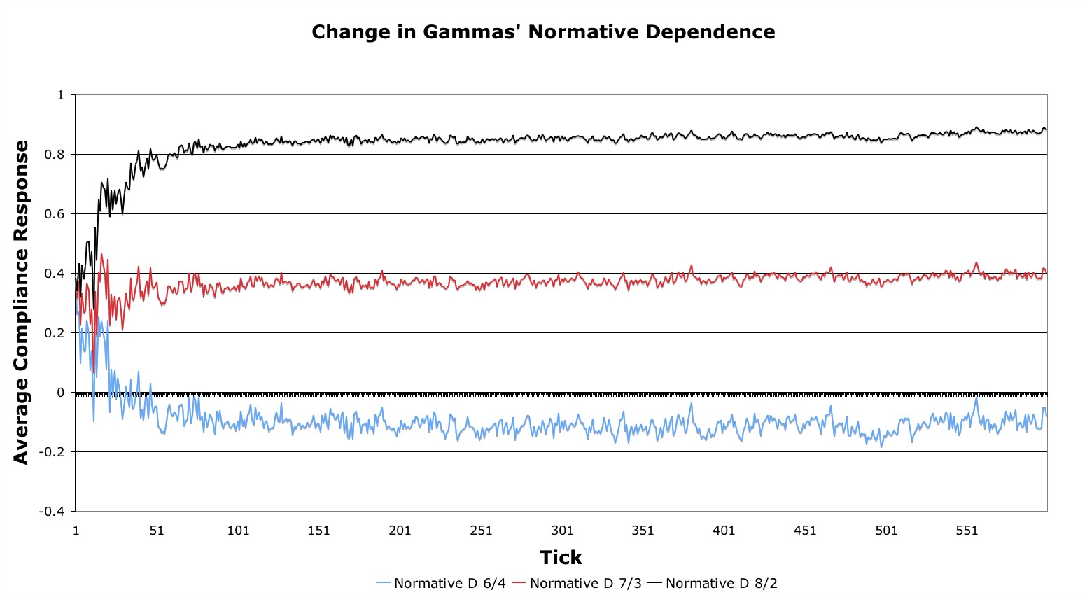
Figure 18. The effect of changing normative dependence on overall compliance in Scenario 5 Scenario 6a-g
- 4.10
- For our final scenario, we attempted to determine the
effect of variations in affective dependence on the overall system. As
before, we use the inputs from Scenario 2, but we only change the
affective dependence values for γ-agents. From the results, overall
compliance is more negative than Scenario 2's parameter states. With
affective dependence ratios ranging between 7/3 to 4/6 (i.e., Scenarios
6a-d) in γ-agents, β-agents are significantly less compliant. What is
interesting to note is as values decrease less than 4/6, then mean
compliance improves, albeit at a very moderate rate (Scenarios 6d-g;
Figure 19). Qualitatively, compliance is strongly negative in values
ranging between 1/9 and 7/3. The results could be explained by the fact
that the decision cost remained at a relatively high level for
γ-agents, while γ-agents' shares in the collective benefit were
relatively low. This leads to the question, can changes in decision
cost and affective dependence in γ-agents create a stronger positive
compliance than only changing the decision cost value?
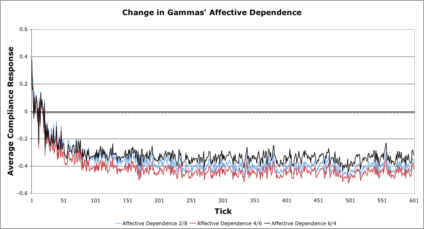
Figure 19. Average compliance responses based on changes in affective dependence Scenario 6h
- 4.11
- In order to show how decision cost suppresses positive compliance, we set the decision cost parameter for γ-agents to 0.4, a value that was earlier used in Scenario 4b. In addition, we use the 1/9 ratio for affective dependence in γ-agents that was modeled in Scenario 6g. In this case, looking at the mean compliance in this scenario vs. Scenario 4b's mean compliance, the overall compliance in this scenario is greater. The distributions of these scenarios are significantly different (i.e., p-value < 0.01). What this shows is that lowering affective dependence values in γ-agents only improves average compliance if decision costs for γ-agents are also lowered.
Discussion
- 5.1
- From these results, we demonstrate two different social network structures (Scenarios 1-2) that have influenced decisions on potable water access. Our model, though still relatively simple, has similarity to observed field observations presented in these scenarios. In addition, we provided several sensitivity tests (Scenario 3-6) of important parameters in γ-agents, testing importance, decision cost, and normative and affective dependence, in order to present how changes in these parameters affect community decisions. The results indicate which thresholds in γ-agent's parameters cause system-level changes that are significantly different than other scenarios. In some cases, although statistical significance was apparent, the compliance result was not qualitatively different than the scenario being compared to (e.g., 6b-g). In other cases, such as in Scenario 5b, a small change to a parameter did cause statistically and qualitatively significant results.
- 5.2
- Currently, ATM is not intended to determine exact choices
specific people make within a decision group. Rather, it is intended to
forecast compliance trends for the group as a whole based on the
influence and overall composition of individual types in community
councils. In other words, the intention is to determine which groups of
decision makers, based on the types of individuals that makeup these
groups, are more likely to be successful in passing measures that
promote resilience to change in water resources. Our attempt can be
summarized as a first step that provides a working model to explain
community decision-making related to water resources. The question
asked at the beginning:
How do gamma agents affect decisions made by community councils in passing resolutions that benefit a village's collective access to clean freshwater?
can be answered to some extent. In Scenario 1, which incorporates Table 1's social network, model output indicates that decision makers may have difficulty forming a consensus, with compliance and noncompliance being almost evenly split. In this village, problems associated with enforcing decisions have been observed, suggesting village council decisions have been weakly enforced or follow-up decisions were not made to sustain initial decisions. In Scenario 2, which applies Table 2's social network, both qualitative observations and model output suggest that the council is generally unable to pass resolutions that a majority of decision makers can accept. - 5.3
- In addition to Scenarios 1 and 2, the parameter sensitivity
tests help to indicate that ATM did function according to our intention
and how changes to γ-agents' parameters affect overall compliance.
Based on the results from all scenarios, we have demonstrated that
γ-agents can negatively or positively affect overall community
compliance based on their levels of importance to the community,
personal decision cost, how they learn from other agents, and
self-oriented goals. Depending on changes to these variables, γ-agents
can direct or deflect β-agents' decisions, thereby influencing the
overall community decision on a given issue. Because β-agents makeup
the majority of community decision makers, α- and γ-agents compete for
these agents, with social influence and agent-specific factors (e.g.,
decision cost and group- vs. self-oriented goals) affecting β-agents'
choices. Minimizing the social significance and agent-specific factors
affecting γ-agents' refusal to comply increases the likelihood that
α-agents can attract β-agents into complying with a choice.
Future Direction and Shortcomings
- 5.4
- For now, the most significant shortcoming of our work is a lack of detailed quantitative validation. However, a benefit to ATM is that it provides questions that we can attempt to address through fieldwork. This can address several possible shortcomings in our work, thereby enhancing validation of ATM. First, collection of similar data to those presented at other villages can assist in showing if ATM is applicable to other cases or what other factors are affecting group decisions. Second, variables such as decision cost, importance, affective dependence, and normative dependence are currently static for agents. This leads us to ask whether or not dynamic processes can be observed evolving these factors in agent decisions, and if algorithms addressing how these variables evolve can be incorporated. Third, we need to obtain more detailed information from specific agents to enhance our understanding not only of how α-, β-, and γ-agents are different from each other but also within each type. For instance, one may expect decision cost values to be different between β-agents. Fourth, we need to collect more precise data on water resource decisions, such as data on specific votes by individuals or how measures implementing previous decisions were stopped, so that quantitative validation can be done on model outcomes. Although we do not intend to forecast precise decision results (i.e., vote results) from our model, we will need to obtain specific decision results in order to conduct quantitative validation. Our future proposed work will not significantly complicate ATM; however, we intend to provide a better understanding of current variables.
- 5.5
- As for factors that might be difficult to determine
regardless of our efforts, we do not know what the social structures
were in villages during the more distant past. The initial social
networks presented have emerged from structures influenced by both
exogenous and endogenous factors, many of which are unknown. There
could be factors from previous decisions that influence current council
decisions in communities; these factors could be difficult for
outsiders to these villages to understand and observe.
Conclusion
- 5.6
- Despite these shortcomings, we feel that models addressing group decision-making are vital for northern latitudes as communities in these regions are undergoing rapid change (Robards and Alessa 2004). Knowing how communities will respond, adapt, and the likelihood of their success in adaptation to such change will increasingly become more important to both aid and management agencies. As researchers, our intent is to assist in this process by creating tools that can enhance decision-making and policy by stakeholders. Some initial progress has been made through ATM by showing that some generally accurate forecasts of village responses can be made. Our objective is that future effort will supplement and enhance our preliminary work.
Appendix
A
-
Model Detail
- A.1
- ATM can be run for as many ticks as desired. For current
scenarios, the number of ticks is set to 600 as it is enough to enable
clear network patterns to develop and accounts for deliberations during
the period in which decisions are made. In the first step of ATM, a
principal component analysis (PCA) is applied on agent weight values to
determine how close agents are to each other in sociometric space (Bonacich 1972; Scott 2000; Kitts 2006). In other words,
weight values distinguish the influence of agents on each other. The x
and y coordinates are the first two eigenvectors of an agent's location
in relation to other agents, based on social weight, applied in a
similar manner as Faust et al. (2002)
and Kitts (2006). The
coordinates provide a visual representation to indicate, based on
social weights, if cliques of agents can be discerned. In the last tick
of a simulation, the PCA is called again after the last model function
in order to provide final output of an agent's sociometric location. A
schematic representation of ATM is provided (Figure 20). We present AT
M based on the order in which main functions are called, with
subfunctions presented after each higher-order function.
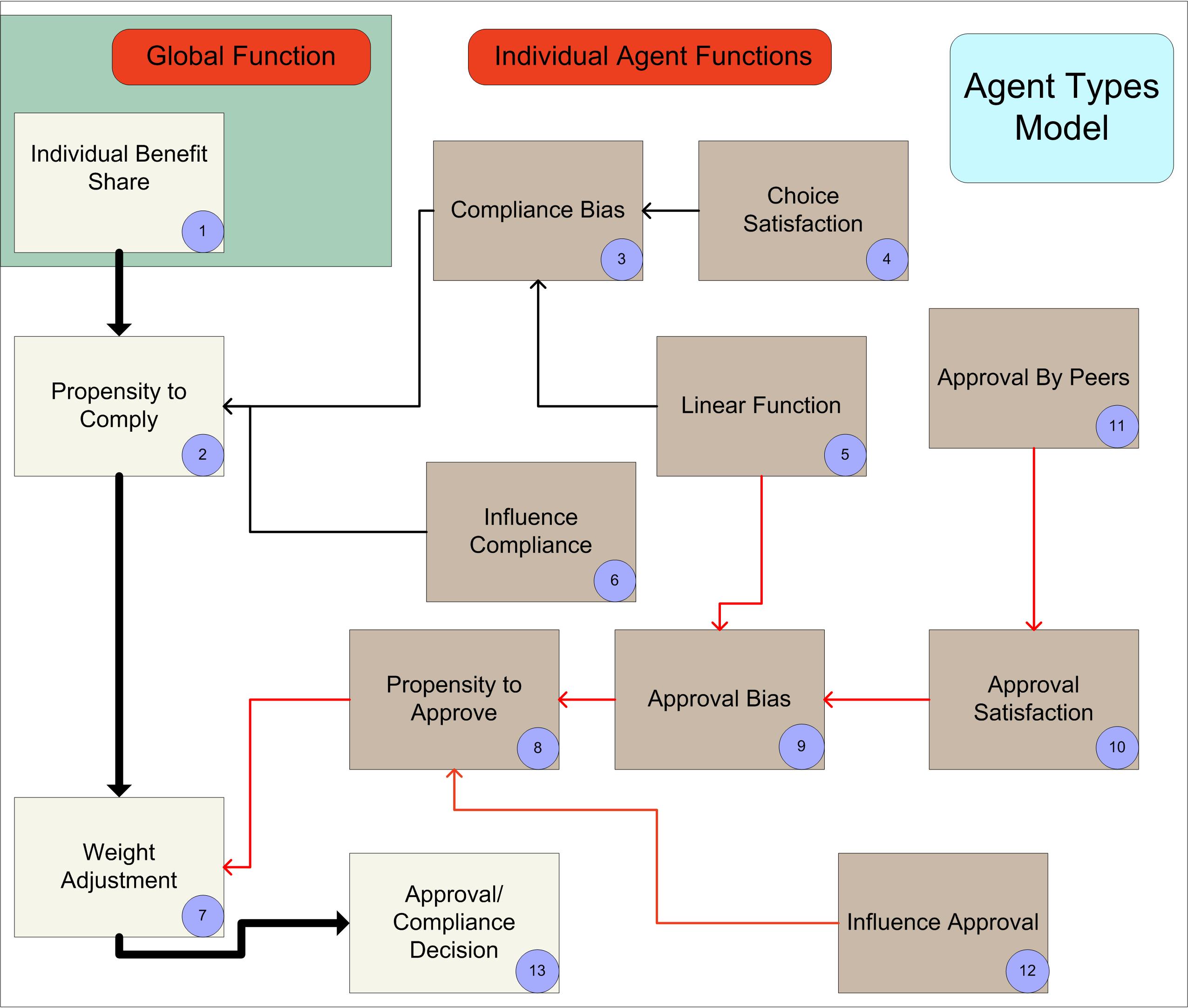
Figure 20. Schematic representation of ATM. Each numbered step corresponds to the numbered function discussed in the text. The main functions are connected by arrows, while subfunctions (shown in brown) are associated with the main functions via colored (black=Propensity to Comply; orange=Weight Adjustment) connectors. Individual Benefit Share
- A.2
- For all ticks, after the PCA is called, the individual
benefit share (S), or individual share of the
collective benefit in Kitts' terminology, within the group is
determined:

where all previous compliance (c) to a choice, with -1 and 1 representing noncompliance and compliance respectively, by each agent (i) are summed and divided by the total number of agents (N). The value provides agents with an idea of how strongly a choice is supported by the decision group and how much benefit agents can expect to receive from the choice. With the benefit share kept as a global variable for the given round, each agent then adjusts his or her propensity to comply (PC), that is whether or not the agent will accept the proposed choice. For all α-agents, their propensity to comply is always 1, as these agents initiate the idea to accept a given choice and never change their minds.
Propensity to Comply
- A.3
- For all other agents, PC is expressed
as:

where δ is the normative dependence, CB is compliance bias, and IC is influence compliance for i. Normative dependence ranges between 0 to 1; values closer to 0 represent those who consider individual experience in learning, while values closer to 1 represent individuals who consider corporate experience in learning (Kitts 2006). This function effectively allows agents to consider individual and group influences in evaluating a choice.
Compliance Bias
- A.4
- Compliance bias can be defined as a dynamic function based
on the previous compliance bias output:

as i's compliance bias is changed (δ) at each tick according to the agent's choice satisfaction (CS), with values limited to being between -1 to 1 (-1 is dissatisfied; 1 is satisfied), and a linear impact function (θ), which allows the compliance bias from the previous tick to influence the current bias. Values greater than 0 indicate greater bias for i to accept a choice. If there is no previous compliance bias, then the previous value is set to 0.
Choice Satisfaction
- A.5
- Choice satisfaction can be defined as:

with affective dependence (D), ranging between 0 and 1, compliance (c), individual benefit share (S), and individual cost (e) to agree on a choice for i as factors in determining choice satisfaction. Affective dependence (D) can be defined as a static variable that captures whether an agent cares more about collective benefit (i.e., values closer to 0) or personal approval (i.e., values closer to 1; Kitts 2006). The individual cost to agree (e) is another agent static value that measures how much cost, or perceived cost, is it for an agent to comply with the decision that is being evaluated. In this function, compliance satisfaction values less than -1 or greater than 1 are artificially made to be -1 or 1 respectively because these extremes represent the most an agent can be dissatisfied or satisfied. In summary, agents consider their collective and individual benefits relative to the decision cost in determining how satisfied they are with accepting a given choice.
Linear Function
- A.6
- In an earlier function (3), the linear impact function (θ(CBi))
was indicated, which can be expressed as:

in which the input value (v) is evolved according to the rule defined. For compliance bias, this allows the previous round's output (i.e., the input value for the function) to influence the current round's consideration, allowing agent experience to affect decisions in a similar conceptual manner to other reinforced learning methods (Macy and Flache 2002). In future efforts, the 0.1 value in the conditional statement could be made more variable to allow for a modification of this rule.
Influence Compliance
- A.7
- In (2), the function for influence compliance (IC)
for i was called. This can be defined as:

where the function evaluates the social weight (w) of i with other agents (j) as well as those agents' importance (I) and choices (c) in influencing i. Variable I ranges between 0 and 1 (0 is no importance; 1 is the most importance), reflecting the influence that an agent has on the overall community. In other words, even if i does not get along with j, i still considers j's overall importance to the community (i.e., global influence on the community). As an example, an agent who holds a critical office or work responsibility in a community (e.g., water system manager) might not be well respected, thus initially having relatively low social weight values with other agents, but that agent may have significant importance due to his or her social position in the community. Our concept of influence departs from Kitts' model in that agents have global influence rather than only local social influence (i.e., social weight). We see an agent's importance as a critical variable in pushing agent choices in communities studied. For this function, the average taken of all the agents excludes i. For future iterations of this model, and as better data emerge, an agent-specific weight value could be used to modify the significance of the importance variable for different agents evaluating influence compliance. After an agent applies the functions discussed (1-6), social weight of i with j is updated.
Weight Adjustment
- A.8
- The basic function for this weight adjustment can be
defined as:
where the change of weight (δW) of i with j evolve using the previous tick's weight (wij). Here, we again depart from Kitts' model in that our agents consider propensity to choose measured relative to j's choice, approval of j based on affective dependence, previous social weight with j, and propensity to approve measured relative to the approval of other agents (k) to j considered as the four factors that evolve the social weight between i and j. In addition to previously defined inputs, one of the subfunctions called is the propensity to approve (PA) of another agent in the social network.
Propensity to Approve
- A.9
- Propensity to approve is defined as:

where AB is approval bias and IA is influence approval of the i and j link. Structured similarly to the propensity to comply function, this function determines the likelihood i will approve of j.
Approval Bias
- A.10
- Approval bias can be expressed as:
which determines the change (δ) from the previous interval's approval bias of i and j, with AS representing approval satisfaction. Values greater than 0 indicate a greater bias to approval of j, while values less than 0 represent a bias to disapprove. The previous step's approval bias, similar to the compliance bias function (3), is used as input for the linear impact function defined earlier (5). This allows previous experience to affect current perceptions.
Approval Satisfaction
- A.11
- Approval satisfaction can be defined as:

with the effective dependence (D) of i, in a similar manner to (4), again used. Agents find values above 0 to be satisfying, whiles values less than 0 are not satisfying. As with choice satisfaction, agents consider group benefit and individual approval in determining their satisfaction. Similar to compliance satisfaction, approval satisfaction values less than -1 and greater than 1 are made to be -1 and 1 respectively because these values represent the extremes of how much an agent is dissatisfied or satisfied in approving of another agent.
Approval by Peers
- A.12
- Approval by peers, as called in (10), can be defined as:

with the function valuing j's approval of i as well as i's weight with j.
Influence Approval
- A.13
- The last relevant function in determining the change of
weight in the i-j link is influence approval (IA),
which can be defined as:

with all the variables applied defined previously. Similar to influence compliance, importance (I) and social weight (w) allow i to consider local and global factors of k in addition to k's approval of j.
Approval
- A.14
- After social weight has been updated, the next method sets
whether i approves of j by
taking the result of PAij. Values
greater than 0.2 automatically result in the i-j
link having approval (i.e., value of 1), while values less than -0.2
show disapproval (-1). In all other cases, the values are evaluated
stochastically via the rule:

where a random value (r) from a uniform distribution (U) between -1 to 1 is evaluated against the PAij value (x). This allows strong negative or positive results to be negative or positive respectively. Other values, however, are more ambiguous and are, therefore, evaluated stochastically.
Compliance Decision
- A.15
- After all agents have finished updating their new weight values and determined whether they approve or reject another agent (j), agents update their compliance decision using the result of PCi. All α-agents retain a response of 1 (i.e. comply), while other agent types with values less or greater than -0.2 or 0.2 respectively result in a deterministic answer in a similar manner to PAij. Results between -0.2 and 0.2 are determined stochastically using the rule in (13).
Appendix
B
- A.16
- Data listed below show scenario metrics including scenarios
compared to each other, the variables tested, the W and p-value
quantities using Wilcoxen signed-rank tests, standard deviation (s.d.),
and mean. Wilcoxen signed-rank tests were used to check statistical
significance between the compliance distributions compared in
scenarios. The p-values listed display results to the nearest 1/100th
value. Each scenario was executed 1000 times. Standard deviation and
mean reflect results from aggregate simulation runs in scenarios. Data
presented as ratios (e.g., 7/3) represent the alpha (i.e., 7) and beta
(i.e., 3) inputs used for a beta distribution.
Scenario Scenario Comparison Variable Tested W p-value S.D. Mean Scenario 1 0.0635 -0.0147 Scenario 2 Scenario 1 vs. Scenario 2 308093.0 0 0.0601 -0.0906 Scenario 3a Scenario 2 vs. Scenario 3a Importance=0.7 107750.0 0 0.0662 -0.0565 Scenario 3b Importance=0.7 vs. Importance=0.6 Importance=0.6 53215.0 0 0.0652 0.0281 Scenario 3c Importance=0.6 vs. Importance=0.5 Importance=0.5 103057.5 0 0.0688 0.0785 Scenario 3d Importance=0.5 vs. Importance=0.4 Importance=0.4 106726.5 0 0.0718 0.1306 Scenario 4a Scenario 2 vs. Scenario 4a Decision Cost=0.5 16136.0 0 0.0547 0.0292 Scenario 4b Decision Cost=.5 vs. Decision Cost=0.4 Decision Cost=0.4 1757.0 0 0.0380 0.2976 Scenario 4c Decision Cost=.4 vs. Decision Cost=0.3 Decision Cost=0.3 537.0 0 0.0289 0.4807 Scenario 4d Decision Cost=.3 vs. Decision Cost=0.2 Decision Cost=0.2 2809.5 0 0.0267 0.5797 Scenario 5a Scenario 2 vs. Scenario 5a Normative Dependence=6/4 197156.0 0.01 0.0644 -0.0941 Scenario 5b Scenario 2 vs. Normative Dependence=7/3 Normative Dependence=7/3 617.0 0 0.0315 0.3701 Scenario 5c Normative Dependence=6/4 vs. Normative Dependence=7/3 Normative Dependence=7/3 537.0 0 Scenario 5d Normative Dependence=7/3 vs. Normative Dependence=8/2 Normative Dependence=8/2 2167.5 0 0.0769 0.832 Scenario 6a Scenario 2 vs. Scenario 6a Affective Dependence=7/3 344259.5 0 0.0790 -0.247 Scenario 6b Affective Dependence=7/3 vs. Affective Dependence=6/4 Affective Dependence=6/4 309761.5 0 0.0860 -0.3153 Scenario 6c Affective Dependence=6/4 vs. Affective Dependence=5/5 Affective Dependence=5/5 300463.5 0 0.0952 -0.3797 Scenario 6d Affective Dependence=5/5 vs. Affective Dependence=4/6 Affective Dependence=4/6 249163.5 0 0.1027 -0.4086 Scenario 6e Affective Dependence=4/6 vs. Affective Dependence=3/7 Affective Dependence=3/7 166257.0 0.02 0.1030 -0.4029 Scenario 6f Affective Dependence=3/7 vs. Affective Dependence=2/8 Affective Dependence=2/8 99208.0 0 0.1059 -0.3589 Scenario 6g Affective Dependence=2/8 vs. Affective Dependence=1/9 Affective Dependence=1/9 81353.0 0 0.1009 -0.3 Scenario 6h Scenario 4b vs. Affective Dependence=1/9 and Decision Cost=0.4 Affective Dependence=1/9 and Decision Cost=0.4 59570.5 0 0.0399 0.3429
Acknowledgements
- All authors (Altaweel, Alessa, and Kliskey) contributed equally to this paper. We are grateful to the National Science Foundation (OPP Arctic System Science #0327296 and #0328686 and Experimental Program to Stimulate Competitive Research #0701898) for funding this research. The views expressed here do not necessarily reflect those of the National Science Foundation.
References
- ALESSA, Lilian N. and Andrew D.
Kliskey (2010) The role of agent types in detecting and responding to
environmental change. Resilience and Adaptive Management
Group Publications 2010(1).
http://ram.uaa.alaska.edu/Publications/AgentTypes.pdf.
ALESSA, Lilian N., Andrew D. Kliskey, Robert Busey, Larry Hinzman., and Daniel White (2008) Freshwater Vulnerabilities and Resilience on the Seward Peninsula as a Consequence of Landscape Change. Global Environmental Change, 18, pp. 256-270. [doi:10.1016/j.gloenvcha.2008.01.004]
BONABEAU, Eric (2002) Agent-based Modeling: Methods and Techniques for Simulating Human Systems. Proceedings of the National Academy of Sciences USA, 99(3), pp. 7280-7287. [doi:10.1073/pnas.082080899]
BONACICH, Phillip (1972) Factoring and Weighting Approaches to Status Scores and Clique Identification. Journal of Mathematical Sociology, 2, pp. 113-200. [doi:10.1080/0022250X.1972.9989806]
CAMERER, Colin F. (2003) Behavioral Game Theory: Experiments in Strategic Interaction. Princeton: Princeton University Press.
EGÍLUZ, Victor, Martin G. Zimmermann, Camil J. Cela-Conde, and Maxi S. Miguel (2005) Cooperation and the Emergence of Role Differentiation in the Dynamics of Social Networks. American Journal of Sociology, 110(4), pp. 977-1008. [doi:10.1086/428716]
FAUST, Katherine, Karin E. Willert, David D. Rowlee, and John Skvoretz (2002) Scaling and Statistical Models for Affiliation Networks: Patterns of Participation among Soviet Politicians during the Brezhnev Era. Social Networks, 24(3), pp. 231-259. [doi:10.1016/S0378-8733(02)00005-9]
FEHR, Ernst and Klaus M. Schmidt (2006) The Economics of Fairness, Reciprocity and Altruism: Experimental Evidence and New Theories. In: S.C. Kolm and J.M. Ythier (Eds.), Handbook of the Economics of Giving, Altruism and Reciprocity, Vol. 1., pp. 616-690, New York: Elsevier.
FLEISCHMANN, Anslem (2005) A Model for a Simple Luhmann Economy. Journal of Artificial Societies and Social Simulation 8(2)4 https://www.jasss.org/8/2/4.html.
GARSON, David G. (1998) Neural Networks: An Introductory Guide for Social Scientists. London: Sage Publications.
HEBB, Donald O. (1949) The Organization of Behavior: A Neuropsychological Approach. New York: Wiley.
HINZMAN, L., N.D. Bettez, W.R. Bolton, S.F. Chapin, F.S. Dyurgerov, G. Fastie, B. Griffth, R.D. Hollister, A. Hope, H.P. Huntington, A.M. Jensen, G.J. Jia, T. Jorgenson, D. Kane, D. Klien, G. Kofinas, A. Lynch, A. Lloyd, A.D. McGuire, F.E. Nelson, W.C. Oechel, T. Osterkamp, C.M. Racine, V.E. Romanovsky, R.S. Stone, D.A. Stow, M. Strum, C.E. Tweedie, G.L. Vourlitis, M.D. Walker, D.A. Walker, P.J. Webber, J.A. Welker, K.S. Winker, and K. Yoshikawa (2005) Evidence and Implications of Recent Climate Change in Northern Alaska and Other Arctic Regions. Climatic Change, 72, pp. 251-298. [doi:10.1007/s10584-005-5352-2]
HOLLAND, John H. (1998) Emergence: From Chaos to Order. Oxford: Oxford University Press.
HOPFIELD, John J. (1982) Neural Networks and Physical Systems with Emergent Collective Computational Abilities. Proceedings of the National Academy of Sciences USA, 79(8), pp. 2554-2558. [doi:10.1073/pnas.79.8.2554]
KITTS, James A. (2006) Social Influence and the Emergence of Norms Amid Ties of Amity and Enmitty. Simulation Modelling Practice and Theory, 14, pp. 407-422. [doi:10.1016/j.simpat.2005.09.006]
MACY, Michael W. and Robert Willer (2002) From Factors to Actors: Computational Sociology and Agent-Based Models. Annual Review of Sociology, 28, pp. 143-166. [doi:10.1146/annurev.soc.28.110601.141117]
MACY, Michael W. and Andreas Flache (2002) Learning Dynamics in Social Dilemmas. Proceedings of the National Academy of Sciences USA, 99(3), pp. 7229-7236. [doi:10.1073/pnas.092080099]
MARWELL, Gerald and Pamela Oliver (1993) The Critical Mass in Collective Action: Studies in Rationality and Social Change. Cambridge, MA: Cambridge University Press.
MIDGLEY, David, Robert Marks, and Dinesh Kunchamwar (2007) Building and Assurance of Agent-Based Models: An Example and Challenge to the Field. Journal of Business Research, 60(8), pp. 884-893. [doi:10.1016/j.jbusres.2007.02.004]
NEWMAN, Mark E.J. and Juyong Park (2003) Why Social Networks Are Different from Other Types of Networks. Physical Review Online Archive, 68(3), 036123. [doi:10.1103/physreve.68.036122]
NORTH, Michael J. and Charles M. Macal (2007) Managing Business Complexity: Discovering Strategic Solutions with Agent-Based Modeling and Simulation. New York: Oxford University Press.
PAHL-WOSTL, Claudia (2002) Towards Sustainability in the Water Sector: The Importance of Human Actors and Processes of Social Learning. Aquatic Sciences: Research Across Boundaries, 64(4), 394-411. [doi:10.1007/PL00012594]
PÉREZ, Raúl L. (2009) Followers and Leaders: Reciprocity, Social Norms and Group Behavior. The Journal of Socio-Economics, 38(4) 557-567. [doi:10.1016/j.socec.2008.05.011]
PUJOL, Joseph M., Andreas Flache, Jordi Delgado, and Ramon Sangüesa (2005) How Can Social Networks Ever Become Complex? Modelling the Emergence of Complex Networks from Local Social Exchanges. Journal of Artificial Societies and Social Simulation 8(4)12 https://www.jasss.org/8/4/12.html.
R Project (2009) The R Project for Statistical Computing. http://www.r-project.org/.
REPAST (2009) Repast: Recursive Porous Agent Simulation Toolkit. http://repast.sourceforge.net/.
RIORDAN, Brian, David Verbyla, and David McGuire (2006) Shrinking Ponds in Subarctic Alaska Based on 1950-2002 Remotely Sensed Images. Journal of Geophysical Research, 111, (G04002), doi:10.1029/2005JG000150. [doi:10.1029/2005JG000150]
ROBARDS, Martin and Lilian Alessa (2004) Timescapes of Community Resilience and Vulnerability in the Circumpolar North. Arctic, 57(4), pp. 415-427. [doi:10.14430/arctic518]
SCOTT, John (2000) Social Network Analysis: A Handbook. 2nd ed. Colchester, UK : Sage Publications.
STOCKER, Rob, David Cornforth, and T.R.J. Bossomaier (2002) Network Structures and Agreement in Social Network Simulations. Journal of Artificial Societies and Social Simulation 5(4)3 https://www.jasss.org/5/4/3.html.
STOCKER, Rob, David G. Green, and David Newith (2001) Consensus and Cohesion in Simulated Social Networks. Journal of Artificial Societies and Social Simulation 4(4)5 https://www.jasss.org/4/4/5.html.
SHUGUANG, Suo and Yu Chen (2008) The Dynamics of Public Opinion in Complex Networks. Journal of Artificial Societies and Social Simulation 11(4)2 https://www.jasss.org/11/4/2.html.
YANG, LU and Nigel Gilbert (2008) Getting Away from Numbers: Using Qualitative Observation for Agent-Based Modeling. Advances in Complex Systems, 11 (2), pp. 1-11. [doi:10.1142/s0219525908001556]