©Copyright JASSS

JASSS logo ----

Richard Vidgen and Julian Padget (2009)

Sendero: An Extended, Agent-Based Implementation of Kauffman's NKCS Model

Journal of Artificial Societies and Social Simulation 12 (4) 8
<https://www.jasss.org/12/4/8.html>

For information about citing this article, click here

Received: 12-Oct-2008    Accepted: 21-Jun-2009    Published: 31-Oct-2009

PDF version


* Abstract

The idea of agents exploring a fitness landscape in which they seek to move from 'fitness valleys' to higher 'fitness peaks' has been presented by Kauffman in the NK and NKCS models. The NK model addresses single species while the NKCS extension illustrates coevolving species on coupled fitness landscapes. We describe an agent-based simulation (Sendero), built in Repast, of the NK and NKCS models. The results from Sendero are validated against Kauffman's findings for the NK and NKCS models. We also describe extensions to the basic model, including population dynamics and communication networks for NK, and directed graphs and variable change rates for NKCS. The Sendero software is available as open source under the BSD licence and is thus available for download and extension by the research community.

Keywords:
Coevolution, Agent-Based Modelling, NK, NKCS, Fitness Landscape

* Introduction

1.1
In the NK model Kauffman (1993; 1995) uses Sewell Wright's (1932) idea of a fitness landscape in which agents seek to move from "fitness valleys" to higher "fitness peaks". At higher points in the landscape survival is more likely and the risk of extinction reduced. In the NKCS model Kauffman extends the NK fitness landscape to coupled landscapes in which a move by one species deforms the fitness of other linked species in the ecosystem, i.e., the species coevolve. Ehrlich and Raven (1964) introduce the term coevolution and use it to describe the reciprocal evolution that results from the interactions of unrelated species. They illustrate coevolution by looking at the interactions between the feeding habits of butterßy larvae and the defences of plants and argue that the coevolutionary process has contributed to a wide diversification of both plants and herbivores. Adaptive agents tend to alter their structures or behaviours as responses to interactions with other agents and the environment. These different species coexist in an ecosystem in which adaption by one type of entity alters the fitness of other types of entity, i.e., action is reciprocal. The actions of one species affects the fitness landscapes of the species to which it is linked and thus the fitness of the different species is constantly changing and deforming.

1.2
Kauffman's NK model (1993) was originally conceived as a means of exploring, through parameter variation, the correlation of fitness landscapes in biological evolution and speciation. In The Origins of Order (1993), Kauffman only describes the NK Model in the biological context for which he designed it and not as the generic model he also claims it may be. However, in the years since, the NK model has become a common tool in the exploration of biological evolution and more recently popular with business researchers applying it to many areas of organizational research including organizational survival on rugged landscapes (Levinthal 1997), situated learning theory (Yuan and McKelvey 2004), manufacturing strategies (McCarthy 2002), strategic imitation (Rivkin 2000), and management accounting systems (Jermais and Gani 2004). In comparison, there is relatively little published about the potentially more interesting coevolutionary NKCS model, notable exceptions being Kauffman's collaboration on a study of group and organizational performance (Levitan et al. 1997) and in the computational field a study of meme-gene coevolution (Bull et al. 2000).

1.3
Various researchers have implemented the NK model (e.g. Lazer and Friedman 2006; Merz 2000) but these have little Web visibility and do not appear to be available for community use. We have also been unable to find a generally available implementation of the coevolutionary NKCS model and thus, given our intention to experiment with and extend the NK and NKCS models, we concluded that we should build a new implementation—Sendero—and make it publicly available (Padget and Vidgen 2008). The primary outcome of our work is, we believe, a well-structured, maintainable, reasonably efficient (inasmuch as the base code is Java) object-oriented solution, embedded in the widely distributed and popular Repast (North et al. 2006) agent-based simulation environment. A second contribution is that the implementation has been validated in, as far as we can tell, the only way possible: by demonstrating functional equivalence to earlier published results for NK and NKCS. The third contribution is the development of NK and NKCS extensions based on suggestions made by other researchers (e.g., Yuan and McKelvey 2004) and our own research agenda. We hope that taken together, this material will make it possible to establish the utility of the NK and the NKCS model by providing a functional framework for community-validated experimentation.

1.4
The remainder of the paper is laid out as follows. In section 2, we describe the essential characteristics of the NK and NKCS models, and in particular the mathematics of landscape construction. We move to the method and implementation issues in section 3 where we outline the way in which we have used agents and the Repast framework to build the new simulation. In section 4 the results are reported for the NK and NKCS models, including docking with Kauffman's original results as reported in Origins of Order. In section 5 we describe the extensions to the NKCS that have been implemented in Sendero and the extensions currently in research and development. We finish with a short summary of the paper.

* The NK and NKCS models

The NK model

2.1
Kauffman (1993) couches the NK model in the language of genetics. An organism has N gene loci and each gene may occur in more than one allele, A. In the simplest case a gene can occur in two alleles, i.e., A = 2. The genotype therefore has N genetic loci, each of which has A alleles, giving a total of AN possible genotypes, which constitute the ensemble (Kauffman 1993, p. 40). Each genotype has N(A—1) one-mutant neighbours; for A = 2, each genotype therefore has N mutant neighbours. The fitness of the genotype is given by the sum of the N independent fitness contributions of the allele at each locus divided by N. The fitness of a given gene depends on its own fitness and on the fitness of some of the other N—1 genes, i.e., the number of epistatic interactions, K.

Figure
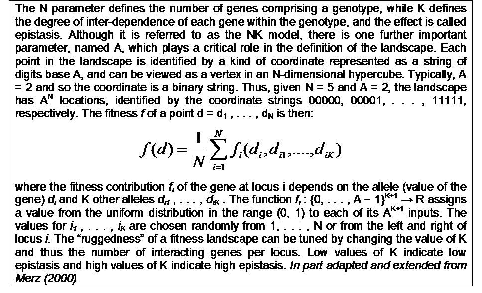
Figure 1. Mathematical formalization of the NK model

2.2
The key parameters in the NK model are, therefore, N, the number of genes in the genotype, and K, the average number of other genes that epistatically affect the fitness contribution of each gene. Assuming, for illustrative purposes, that A = 2 then the NK model works as follows (adapted from Kauffman 1993, p.42): -

2.3
The fitness calculation of Kauffman's NK Model is probably the main justification for its interest. It has been designed to allow the landscape to be changed easily from a rugged uncorrelated landscape to a correlated single peak landscape, by the alteration of a single parameter, K. The mathematical formalization of this is fairly standard and appears in a form similar to that in Figure 1 in several publications.

The adaptive walk

2.4
The purpose of running a simulation is to observe how the agents traverse the landscape seeking higher fitness locations. This means each agent in turn has the opportunity to move from its present location to another location, which in the first instance is taken to be an adjacent location, where adjacent means the coordinate differs in precisely one characteristic. These are known as "one-mutant" neighbours.

2.5
Each site has D = (A – 1)N one-mutant neighbours, for example if A = 2 and N = 5 then D = 5. An agent is initially located at a randomly determined location on the landscape, that is a location in the range 00000 through 11111, such as 01110 for N = 5. The fitness of this location is computed according to the algorithm outlined above and detailed in Figure 1. There are three standard strategies for determining the agent's next location: -

2.6
Once an agent cannot find a fitter neighbouring location it stops walking and stays where it is on a (possibly sub-optimal) local peak. Thus one termination condition for the simulation is when some percentage of, or all, the agents have stopped walking.

The NKCS model

2.7
The NKCS model offers a richer environment than the NK model, by introducing the principle of coevolution. Naturally, it is also significantly more computationally demanding. NKCS is a relatively simple extension of the basic model, because all that is required is the instantiation of multiple coevolutionary sets of species, each acting on their own landscapes, but at the same time affecting the landscapes of others.

2.8
To be more specific, the mathematical formulation states that in a given model, there shall be S coevolving species in total. A further parameter X defines how many species each shall interact with, while C determines the number of genes of other species that shall affect each gene of a given species. This is in contrast to the K parameter of the NK model, which controls internal epistasis, whereas C controls cross-species (external) epistasis.

2.9
In less technical language, the fundamental difference between NK and NKCS is that in the former the agents are unaware of other agents' behaviour, that is, they are all walking the landscape independently. The landscape is fixed and unchanging (although it may be too large to know and to explore fully). In the NKCS model there is a single agent on each landscape and that agent represents the population, as explained in (Kauffman 1995):
We will treat each species as though its entire population were genetically identical. At each "generation", the population will seek a fitter genotype by mutating a single, randomly chosen gene to the alternative allele. If the new mutant genotype is fitter, the population will move to this new point on its landscape. (Kauffman 1995, pp. 225-226)

2.10
The representatives of each species are locked together in a coevolutionary set such that a move by one species deforms the landscapes of its partner species. For example, if there are three species (S = 3) and each species is connected to the other two species (X = 2) then the coevolutionary set would comprise three agents (one per species) whose genes are connected internally through K coupling and externally through C coupling.

2.11
In the NK model agents are independent and in effect move simultaneously; in the NKCS model, however, the species have to move in turn and the movement of each to a fitter location impacts the fitness of those which do not move. In some simulations Kauffman throws 100 coevolutionary sets into the ecosystem and looks at the fraction (percentage) of the pairs still walking at each generation (Origins of Order, Figure 6.3). This is not necessarily equivalent to throwing 100 agents onto an NK landscape (where average fitness of the species is calculated as the average of the fitness of the 100 agents) since in the NKCS model each of the 100 coevolutionary sets represents coupled genotypes, that is, there is a subtle distinction between an instance of a species in the NK model and the coevolutionary set representing a population in the NKCS model.
Example

2.12
Assume that there are two species, s1 and s2 (i.e., S = 2), that each species interacts with one other species (X = 1), and that each characteristic is affected by two other characteristics from the linked species (C = 2). The arrows in Figure 2 indicate that the fitness of gene n2 in s1 depends on the fitness of itself (n2), the fitness of n1 and n3 in s1 (K = 2), and the fitness of n2 in s2 (C = 1). As the values of N, K, and C increase then the complexity of the interactions within the NKCS model rises rapidly.

Figure
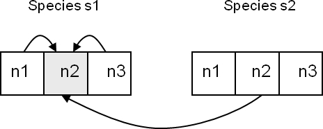
Figure 2. Gene n2 in species s1 depends on n1 and n3 (K = 2) and n2 from species s2 (C = 1)

2.13
Kauffman claims that evolution is always coevolution. However, where species are loosely coupled and the species are robust such that a change in one species does not have much effect on other species then the NK model is a valuable way of exploring how a species can evolve on a fitness landscape. Furthermore, the NK model appears to offer a useful description of real world problems and problem-solving on complex landscapes. In situations where the species are interdependent, such as may be the case for competing organizations in a marketplace or tightly integrated organizations in a supply network, then the NKCS variant offers a way of modeling the dynamics of coevolution. In short, whether it is the NK or the NKCS that is more applicable depends on the situation being modeled and the problem being addressed.

* Method—the Sendero implementation

Implementation strategy

3.1
Given the relatively sparse information describing the specification of the NK and NKCS models, our approach to the implementation was incremental. We first built a basic version of the NK model in order to assess its validity. Having done so, we then attempted to extend our NK model to address the more complex NKCS landscape, using the same techniques wherever possible. The model was implemented using the RepastJ (North et al. 2006) agent-based simulation toolkit. The design principles behind the original implementations of the NK and the NKCS models do not appear to be documented and so this gave us the (relative) freedom to use our imagination about how to realize a system that would demonstrate the behaviour Kauffman describes. Although the abstract genetic model at the heart of NK/NKCS might initially encourage the adoption of a conventional procedural encoding combined with a mechanism for handling varying population sizes, several engineering factors, along with our own pre-disposition to agent-oriented techniques, made it look like an experiment that should be tried, but specifically:
  1. The classical notion of an agent interacting with others via an environment appeared to us to be a very natural target mapping from the entities in Kauffman's design.
  2. Working with an agent-based simulation environment offered an attractive separation of concerns between essentially the model (the agents), the view (the datasets) and the controller (the simulation engine), allowing us to concentrate on the model, albeit countered by the overhead of learning about and working with the simulation framework. That does not mean it was straightforward: the system we describe here is the third version—earlier prototypes were developed in both Mason and in Repast and the current version is a heavily refactored development of the first Repast version.
  3. The modularity enforced by the agent approach, has we believe contributed to the relative ease with which we have been able to extend the NK and NKCS models. How much those benefits are due just to agents or to using a mature framework like Repast is not really worth debating, but by choosing a popular framework, it does in principle also ease access for the wider community.

Implementation method

3.2
The NK model maps onto an agent-based simulation very simply: the agents are the organizations, which move about the landscape with a simple goal of increasing fitness at each generation. In the NKCS model the situation is slightly more complex: within the Repast framework we implemented each coevolutionary set as an agent. These sets contain a number of species, each with its own distinct landscape. At each generation of the simulation, the species take turns to move on their own landscapes, which are perturbed by the movements of the other species in the set. To describe the co-evolutionary process, we collect data at the level of the individual species.

3.3
In designing the NKCS implementation, the validated NK model was refactored to abstract the Organization and FitnessLandscape classes which reflect the extensive commonalities in behaviour between the two models. In particular, from the implementation perspective the calculation of fitness is almost identical between NK and NKCS and is performed by the same method. In both cases, for each characteristic, we build a string representing the state in base A, of the characteristic itself, and the K characteristics which influence it. To extend this to NKCS, we add to the string the states of the C characteristics of each of the X other species to which the species under examination is linked. This string is then assigned a random fitness value and stored.

3.4
Having decided on the specification of the models, a significant challenge was the representation of the fitness landscape itself. In both the NK and NKCS models the landscape possesses a finite number of states (albeit an extremely large number in the case of NKCS). The fitness of agents at given locations is randomly assigned in response to the characteristics of the location (and, for NKCS, the location of other species in the set). To generate random fitness values and landscape locations we used the Colt Mersenne Twister random number generator supplied with RepastJ. At the same time, an agent arriving at a location that it (or another agent) has previously visited must be awarded the same fitness value as reported earlier. Therefore, any location already visited must be remembered rather than recalculated.

Figure
Figure 3. The Sendero parameter interface (generated by Repast)

3.5
We compute and store location fitness values only when they are first visited by an agent (or checked as a possible candidate to be moved to). In this way we avoid the need to store the entire landscape, much of which may never be visited in the course of the simulation. However, saving the fitness values for all of the locations that have been visited or checked for future reference, is we believe an unavoidable cost. This space requirement represents the major constraint on simulation size in our implementation. In runs where the required landscape is large (or numerous landscapes are used, in NKCS), or large numbers of organizations walk extensively on the landscape, we found that gigabytes of memory could be consumed. Further work could attempt to use disc-based storage to offload areas of the landscape as agents become less likely to visit them—although this process is not straightforward.

3.6
All of the NK and NKCS simulations reported here were run on a standard desktop computer. Calculation predominantly occurs in a single thread, so a single batch run does not benefit from a multi-core CPU. Execution time and memory requirements increase significantly for higher values of N and K, but in an approximately linear fashion when larger numbers of agents are released. The longest NK execution reported here is for N = 96 and K=95. Running the NK model for one such organization over 100 runs (and therefore 100 different landscapes) resulted in an execution time of around two and a half minutes (1.55 seconds per run). For comparison, 100 runs for 10 NK organizations with N=96 K=95 took an average of 18.7 seconds per run. This performance suggests the implementation is suitable for running all but the largest simulations on a personal computer. Faster machines with more memory will of course permit the exploration of yet larger regions of the parameter space, but fundamentally the NK model is NP-complete (Weinberger 1996), so the incremental resources cost for each increment in N (and attendant K) will be very high. Since NKCS is an extension of NK, it is clearly in the same complexity class and as our performance figures show, even runs for the same values of N and K take considerably longer for NKCS than NK.

Figure
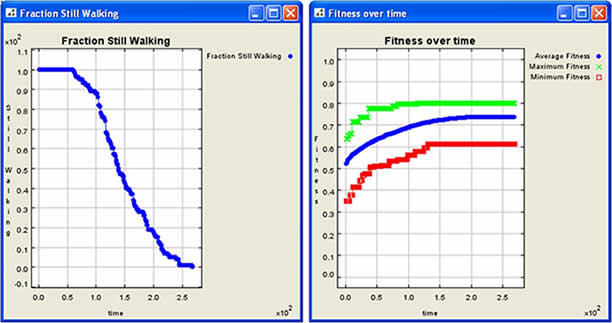
Figure 4. Sample graphical output for Sendero (generated by Repast)

3.7
One of our primary objectives in re-engineering the model(s) was to allow for future flexibility and extensibility. In the absence of a detailed specification (especially in the case of NKCS), we allowed for adjustment of numerous aspects of the model not discussed here due to space constraints (see Padget and Vidgen 2008 for documentation). By so doing, we were able to test and refine our assumptions as to the exact workings of Kaufmann's calculations, and also to examine their sensitivity to differing constraints. It is our hope that we and others will be able to extend their capability further. We discuss some possible directions and their applications in section 5.

The Sendero/Repast user interface

3.8
Sendero is run in the Repast environment. Repast builds a parameter interface based on the Repast model (Figure 3) and the user can adjust parameter values, run the model, and view the results in real time. In Figure 4 two of the graphs produced as the model runs are shown, "fraction still walking" and "fitness over time". A similar interface is generated for the NKCS model. For multiple runs it is easier to build files of parameters and to execute the NK and NKCS models in batch mode.

3.9
An executable as well as the complete source code for Sendero are available from the Sendero wiki pages.

* Results

NK results

4.1
Verification of the implementation is a particularly difficult problem, because as noted earlier there appear to be no open-source systems—otherwise we would not have spent time and effort on building this one—and although there are some binaries of uncertain provenance, without the accompanying source code it is not possible to examine the workings of these implementations. Thus, as far as we can tell, the only means to assess the correctness of the simulation is to demonstrate equivalence to the data published in Kauffman (1993). For each combination of N and K (A=2) in Table 2.1 of Origins of Order (p. 55) 100 runs have been conducted and the results averaged. Each individual run has a single agent released at random on to the landscape and the results therefore represent the average of 100 different fitness landscapes.

Figure
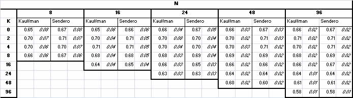
Table 1. Mean fitness of local optima - Kauffman's Table 2.1, p. 55 results compared with Sendero. Note: along the diagonal where K = N, actual value is K - 1

4.2
Kauffman's reported means and standard deviations—to two decimal places as recorded in Table 2.1 of Origins of Order (p. 55)—are shown in Table 1 of this article alongside the results from Sendero. The results are remarkably similar for both means and standard deviations, especially given that Kauffman's simulations were built pre-1993 in an unspecified environment (e.g., we do not know how random fitness values were generated) while Sendero is implemented in an agent-based model. We are therefore confident that Sendero is a faithful implementation of the NK model.

4.3
Clearly, the kind of datasets generated by a NK simulation are not going to reveal much in a plain text format: some form of visualization is needed. To illustrate the properties just discussed, in Figures 5-7 we show graphs of maximum, minimum and average fitness for various combinations of N and K. All graphs represent the average of 100 runs where each run has 100 agents released at random on to the fitness landscape. We can observe that average fitness reaches around 0.66 in the K = 0 case, rises to around 0.7 for K = 4 and then drops to around 0.63 for K = 23.

Figure
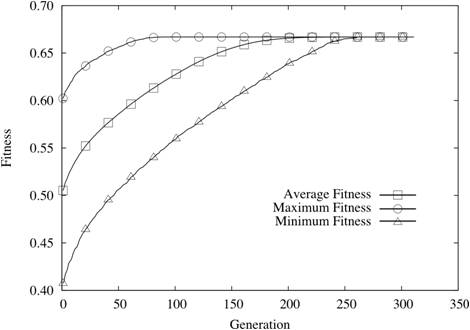
Figure 5. N = 24 and K = 0

Figure
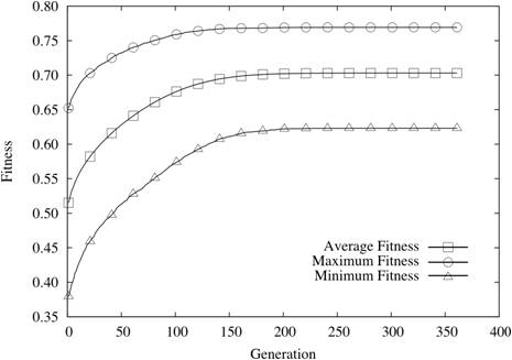
Figure 6. N = 24 and K = 4

Figure
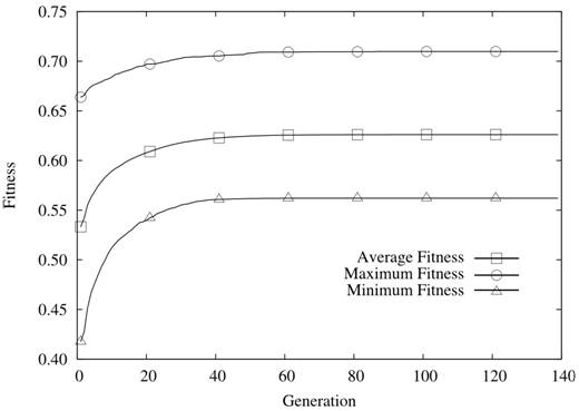
Figure 7. N = 24 and K = 23

Video 1. Shows a population of 100 agents, each with 48 alleles having epistatic interactions with all 47 others, leading to a maximally rugged fitness landscape. Average fitness quickly reaches a local maximum.
(Click on the movie for a larger version in a new window)

NKCS results

4.4
In the NKCS model the walk for the species is fundamentally the same as it is for agents in the NK model. Each genotype looks for a fitter location using the same methods as in the NK model. We illustrate, in Figures 8 and 9, our attempts to dock our NKCS implementation with Origins of Order, Figure 6.3 (p. 247). Like Kauffman, we present the results of a single run with 100 coevolutionary sets for C = 1 and C = 8. Given that a single landscape is used in this simulation the results vary slightly from run to run but visual inspection shows that the results shown in Figures 8 and 9 faithfully replicate Kauffman's findings. Kauffman does not report standard deviations for the NKCS model, being more interested in the behaviour of the model and the identification of emergent regimes: stasis (order), the emergent region of complexity ("edge of chaos"), and the red queen effect (chaos). The pattern of behaviour produced by Sendero is the same as that reported by Kauffman in Origins of Order. When K is low relative to C then the system exhibits chaotic behaviour—each species can move and find improved fitness but in doing so disturbs the landscape of its linked species and thus the species chase ever-receding peaks. When K is high relative to C the system exhibits stasis—the species quickly find local optima and become frozen. In Table 2 we show the fitness values achieved for C = 1 and C = 8 with different values of K. For C = 1, fitness is highest when K = 2 and as K increases (C held constant) fitness falls and the sets stop walking more rapidly as they become frozen on the landscape. For C = 8, fitness is highest when K = 16; when K = 2 none of the sets stop walking and the result is chaos. Kauffman suggests that fitness is greatest for two species where K = C · S, i.e, for C = 1 then K = 2 is optimal and for C = 8, K = 16 is optimal. This is borne out by the simulation results in Table 2.

Figure
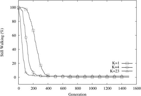
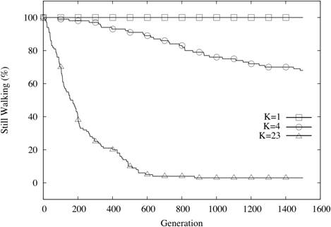
Figure 8. Coevolutionary sets still walking (N=24, C=1, K varies)

Figure
Figure 9. Coevolutionary sets still walking (N=24, C=8, K varies)

Video 2. Shows a population of five co-evolutionary sets, each comprising five species. The fitness of each species within the co-evolutionary set is dependent on interactions with two other species in the set. Fitness of the sets proceeds chaotically at first, before resolving to a stable maximum after 450 generations.
(Click on the movie for a larger version in a new window)

Figure
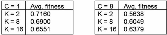
Table 2. Final fitness values for NKCS simulations shown in Figures 7 and 8

4.5
The NKCS coevolutionary model thus produces markedly different results from the NK. In the NK model, a low value of K (typically around 3 or 4) results in the highest average fitness regardless of the value of N, whereas the NKCS model depends on matching K to C.

* Extensions

5.1
We first discuss some extensions to the basic NKCS implementation that are in the first release of Sendero (Padget and Vidgen 2008) and then some of the extensions that are under investigation.

Extensions in the base version of Sendero

Parameters

5.2
A number of enhancements to the basic parameters of the NK and NKCS models have been implemented in Sendero:
Long jumps

5.3
Kauffman introduces a further strategy for an agent that cannot climb any further (that is, it has reached a local maximum): the agent may jump to a new location on the landscape. This works by choosing a location at random, computing its fitness and moving to that location if fitness is higher than the current location. Stopping conditions for the long jump strategy consist of limits on the number of successful jumps, and the number of failed searches for a fitter location. Long jumps prove to be a rather blunt weapon on complex landscapes since the probability of finding a fitter location is low and fitness increases as a result of long jumps are small. A more sophisticated approach would be to adopt a "search party" method where an agent makes a long jump and then conducts a local exploration, returning to its original location if a fitter local peak cannot be found. This is not dissimilar to the communication network (see next), in which agents can move to the location of fitter agents.
Communication networks

5.4
A common problem domain for NK simulations concerns the communication of information between agents, reflecting connectivity such as that found in communities, in the web or in supply chains, for example. Consequently, it is useful to be able to define communication topologies to be able explore scenarios such as that discussed in Lazer and Friedman (2006) who reach the (initially) counter-intuitive conclusion that more communication results in lower overall system performance as a result of a high level of mimicry, while greater (relative) isolation results in higher overall system performance through a higher level of exploration/innovation. Sendero allows communication between agents subject to a selection of connection policies, such as random, fully-connected, small-world or linear networks.
Life and death—population dynamics

5.5
The standard NK simulation allows all the agents created at the start to continue walking until the final tick. A variation of this scenario favours a form of "survival of the fittest", imposing a mechanism for killing-off agents that are not performing well—a model that is quite appealing in market scenarios in which the agents are competing organizations—and creating new agents—new market entrants—at the same time. We have implemented such a policy for managing the agent population that kills off poorly performing agents and creates new ones, keeping the population at a constant level. The user may specify a fitness threshold that is used to decide what action to take; if the difference between an individual agent's fitness and that of the fittest agent exceeds this then it is terminated. A fresh agent is generated either by cloning an existing agent or by selecting a new location at random. The decision of which option to take (i.e., copy an existing agent's location or generate a new location randomly) can also be decided by looking at the genetic load of the landscape.

5.6
Clearly, for the researcher prepared to develop additional code, all kinds of policies and extensions to the Sendero base are feasible.

Extensions developed for further research

Landscape perturbation

5.7
We have begun to investigate the means to incorporate "extreme events" into a NK simulation through perturbations of the landscape. We create a landscape of identical dimensions to the NK landscape featuring a localised disturbance, whose magnitude decreases with distance. We then map this magnitude onto the NK fitness value for the agents' locations—allowing us to observe responses to a sudden localised change in the environment. The disturbances can be run for different values of N and K and with different degrees of disruption to see how well the agents recover following a landscape disaster.
Directed graph of species

5.8
We have introduced a directed graph to the NKCS model to allow species to be coupled explicitly. For example, species might be configured as a chain where each member connects with two neighbours but with no wrap-around. Thus for S = 4 the end species, s0 and s3, have only one connected species (s1 and s2 respectively) while interior chain members have two connections (e.g., s1 connects to s0 and s2). Tuning for different combinations of low and high K and C (internal and external epistasis) gives a surprising range of network behaviours. Different configurations can be built to model supply networks and groups with a central controlling species, and any network that can be configured as a graph. A further extension is to allow C values to be asymmetric, e.g., s1 may depend on C = 5 locations of s2 while s2 depends on only C = 1 location from s1.
Species change rate

5.9
In the basic NKCS model each species moves at each tick. Interesting effects have been reported by Bull et al. (2000) who allow species to move at different rates to simulate the coevolution of memes and genes. For example, species s0 might move on every time tick while species s1 moves on every tenth time tick. This extension is likely to be particularly relevant to organizational coevolution where organizations move and develop at different rates.

* Summary

6.1
Kauffman's NK and NKCS family of fitness landscape models have been adopted by many researchers across many disciplines. To our knowledge, a package—closed or open source—for NKCS simulations is not publicly available and Sendero is thus a step toward the creation of a common good for complexity researchers. It has been difficult to "bottom out" Kauffman's—and other researchers—implementations of NKCS models. This is largely due to the lack of program specifications and details of implementation. By making our assumptions and operational decisions explicit (and ultimately the source code) other researchers can verify, amend, and extend our implementation. Finally, we have shown how the NK and NKCS models can be extended to reflect situations that are closer to real-world organizations.

* References

BULL, L., O. Holland, and S. Blackmore, (2000). On Meme-Gene Coevolution. Artificial Life 6(3): 227-235.

EHRLICH, P. R. and P. H.. Raven, (1964). Butterflies and Plants: A Study in Coevolution. Evolution, 18(4): 586-608.

JERMAIS, J., and L. Gani, (2004). Integrating business strategy, organizational configurations and management accounting systems with business unit effectiveness: a fitness landscape approach. Management Accounting Research, 15: 179-200.

KAUFFMAN, S., (1993). The Origins of Order: Self-Organization and Selection in Evolution. Oxford University Press.

KAUFFMAN, S., (1995). At Home In The Universe. Oxford University Press.

LAZER, D., and A. Friedman, (2007). The social structure of exploration and exploitation. Administrative Science Quarterly 52: 667-694.

LEVINTHAL, D. A., (1997). Adaptation on rugged landscapes. Management Science, 43(7): 934-950.

LEVITAN, B., J. Lobo, R. Schuler, and S. Kauffman, (1997). Evolution of organizational performance and stability in a stochastic environment. Computational & Mathematical Organization Theory, 8: 281-313.

MCCARTHY, I. P., (2002). Manufacturing fitness and NK models. In G. Frizelle and H Richards, editors, Tackling Industrial Complexity. Institute for Manufacturing, Cambridge, UK. Available via www.ifm.eng.cam.ac.uk/mcn/proceedings.htm. Retrieved January 2008.

MERZ, P., (2000). Memetic Algorithms for Combinatorial Optimization Problems: Fitness Landscapes and Effective Search Strategies. PhD thesis, University of Siegen.

NORTH, M., N. T. Collier, and J. R. Vos, (2006). Experiences creating three implementations of the repast agent modeling toolkit. ACM Trans. Model. Comput. Simul., 16(1): 1-25.

PADGET, J., and R. T. Vidgen, (2008). The Sendero Project. On-line access at http://wiki.bath.ac.uk/display/sendero. Retrieved October 2008.

RIVKIN, J., (2000). Imitation of complex strategies. Management Science, 46(6): 824-844.

WEINBERGER, E., (1996). NP Completeness of Kauffman's N-k Model, a Tuneably Rugged Fitness Landscape. Sante Fe Institute working paper 96-02-003. Available via http://www.santafe.edu/research/publications/workingpapers/96-02-003.ps. Retrieved 20090313.

WRIGHT, S., (1932). The role of mutation, inbreeding, crossbreeding and selection in evolution. In Proceedings of the Sixth International Congress on Genetics, volume 1, pages 356-366.

YUAN, Y., and B. McKelvey, (2004). Situated Learning Theory: Adding Rate and Complexity Effects via Kauffman's NK Model. Nonlinear Dynamics, Psychology, and Life Sciences, 8: 65-102.

----

ButtonReturn to Contents of this issue