Nicholas M. Gotts and J. Gary Polhill (2009)

When and How to Imitate Your Neighbours: Lessons from and for FEARLUS

Journal of Artificial Societies and Social Simulation 12 (3) 2
<https://www.jasss.org/12/3/2.html>

For information about citing this article, click here

Received: 29-Jun-2007    Accepted: 16-May-2009    Published: 30-Jun-2009

Abstract

This paper summarises some previously published work on imitation, experimentation (or innovation) and aspiration thresholds using the FEARLUS modelling system and reports new work with FEARLUS extending these studies. Results are discussed in the context of existing literature on imitation and innovation in related contexts. A form of imitation in which land uses are selected on the criterion of their recent performance within the neighbourhood of the land parcel concerned (called here 'Best-mean Imitation'), outperforms comparably simple forms of imitation in a wide range of FEARLUS Environments. However, the choice of criterion is shown to interact with both the way the criterion is applied, and the land manager's aspiration threshold: the level of return with which they are satisfied. The implications of work with FEARLUS for the broader bodies of research discussed, and vice versa, are considered.

Keywords:

Imitation, Innovation, Aspiration, Land-Use, Spatio-Temporal Heterogeneity

Introduction

1.1

To say a decision-maker "imitates their neighbours" underspecifies their procedure. Do they imitate all the time, or only sometimes? Do they rely on the number of neighbours taking each course of action, or imitate the most successful? Whether influenced by quantity or quality (or both), do they select only among the highest-scoring alternatives, or use something like proportional weighting? We show that different approaches can have very different results, and their relative success can depend on the spatio-temporal heterogeneity of the environment, and on what other decision-makers are doing.

1.2

The spread of agricultural innovations is of both scientific and practical interest. Most research examines why apparently beneficial innovations are not adopted (Fujisaka 1994; Cramb et al 1999), or the personal or social factors determining adoption (Feder and Slade 1984), including the "risk aversion" of individuals (Abadi Ghadim and Pannell 1999), and neighbours' influence (Ryan and Gross 1943; Pomp and Burger 1995; Abadi Ghadim and Pannell 1999). The approach taken to modelling risk aversion here derives from the idea of an aspiration level (Simon 1955): the lowest price a seller will accept. Simon (1957) suggested that much human problem-solving relies on satisficing: seeking a good enough solution, then looking no further, thus avoiding further search costs. Satisficing is represented in FEARLUS by giving decision-makers an Aspiration Threshold ^[1] for the economic return on a Land Parcel. If this is achieved, the Land Use on that Parcel will not be changed. Higher Aspiration Thresholds represent lower risk aversion; or a different balance between strategies of exploration (of the set of possible land uses) and exploitation (of the current land use). There may be considerable risk in abandoning what worked well enough last year in pursuit of possible higher returns. Also, there may be significant costs attached to change itself, although FEARLUS does not currently represent such costs.

1.3

This paper summarises some previously published work using the FEARLUS modelling system (Polhill Gotts and Law 2001; Gotts Polhill and Law 2003; Gotts Polhill and Adam 2003; Gotts Polhill, Law and Izquierdo 2003), and reports new work extending and systematising these studies. It discusses FEARLUS work in the context of literature on the role of imitation in land use change and the adoption of agricultural innovations, and work on imitation in spatial games. We show that a form of imitation in which land uses are selected on the criterion of their recent performance within the neighbourhood of the land parcel concerned (called here "Best-mean Imitation"), outperforms comparably simple forms of imitation in a wide range of FEARLUS Environments. However, the choice of criterion interacts with both the way the criterion is applied (whether selection is confined to the highest-scoring alternatives, or uses proportional weighting based on the scores) and land managers' aspiration thresholds. Much work on imitation in a spatial context has adopted particular forms of imitation without considering the range of alternatives. The implications of work using FEARLUS for the broader bodies of research discussed, and vice versa, are considered.

Method

General Description of FEARLUS Models

2.1

A FEARLUS model^[2] consists of a set of Land Managers and their Environment, which includes a grid of Land Parcels, and a set of possible Land Uses. Every Year, Land Managers select a Land Use for each Land Parcel they own. Model parameters also specify External Conditions, representing economic and climatic factors, and encoded as a bitstring, the length of which is a model parameter. This bitstring can vary Year to Year but applies across the whole grid. In most runs discussed, the initial bitstring is determined randomly, and each subsequent bitstring is produced from its predecessor by applying a predetermined Flip Probability ( f) to each bit independently: if f = 0 the initial bitstring will be retained throughout; if f = 1/2, each Year's bitstring is independent of its predecessors and the External conditions are temporally uncorrelated. If 0 < f < 1/2, the External Conditions change, but are temporally correlated. Each Land Parcel also has a bitstring of Biophysical Characteristics, fixed for the duration of a simulation run (again, bitstring length is a model parameter; it is the same for all Land Parcels). There are also two numerical parameters unvarying over space and time (and over Land Managers): a Break Even Threshold, specifying how much Yield must be gained from a Land Parcel to break even, and the Land Parcel Price. These fixed parameters are unrealistic, but reduce the parameter space to be explored; they are key parts of the mechanism allowing the transfer of Land Parcels from less successful to more successful Land Managers.

2.2

In Year 0, Land Parcels are assigned to Land Managers, and there is a random allocation of Land Uses to Land Parcels. Land Managers have an Account, initially set to zero. The rest of the run repeats the following annual cycle:

1. Selection of Land Uses. The Land Use for each Land Parcel is selected by its Land Manager, using the latter's Land Use Selection Algorithm.
2. Determination of External Conditions.
3. Calculation of Yields. The concatenated bitstrings for a Parcel's Biophysical Characteristics and the current External Conditions are matched against one representing the requirements of the current Land Use: the Yield is the number of matching bits.
4. Harvest. The Account of each Land Manager is adjusted. For each Land Parcel owned, that Parcel's Yield is added, and the Break Even Threshold subtracted.
5. Selection of Land Parcels for sale, and retirement of insolvent Land Managers. Each Land Manager in deficit sells Land Parcels as necessary to clear the deficit. Any unable to do this while retaining at least one Parcel, leave the simulation.
6. Land Sales. One ticket in a lottery is issued for each Grid Neighbour of the Parcel belonging to a Land Manager with at least the Land Parcel Price in their Account (a Land Parcel's Grid Neighbours are the eight Parcels orthogonally or diagonally adjacent to it). One ticket is assigned to a potential new Land Manager. A Land Manager must buy the Land Parcel if selected.

2.3

In addition to its Grid Neighbourhood, each Land Parcel has a Social Neighbourhood. This includes all the Land Parcels managed by its own Land Manager, or by any Neighbour of that Land Manager, where two Land Managers are Neighbours if and only if they manage Land Parcels that are Grid Neighbours. Figure 1 illustrates the Grid and Social Neighbourhoods of the central, stippled Parcel: the solid black line bounds the Social Neighbourhood, the dashed line bounds the Grid Neighbourhood (except where overlain by the Social Neighbourhood boundary). For a fuller description of FEARLUS models, see Polhill, Gotts and Law (2001).

Aspiration Threshold Selection Algorithms

2.4

Most of the Selection Algorithms discussed here use an Aspiration Threshold: the Land Manager checks whether the most recent Yield from a Land Parcel met the Threshold and if so, leaves its Land Use unchanged. Otherwise, a Land Use is selected anew (either the same or a different Land Use may be chosen). In the Selection Algorithms focussed on here, this selection process involves either Random Experimentation (a random choice between the possible Land Uses, all having equal likelihood of being selected), symbolised R in what follows, or Imitation, in which the Land Use is selected from among those used in the Parcel's Social Neighbourhood in the preceding Year. Note that the Aspiration Threshold has a completely different role from the Break Even Threshold. The latter is a property of the Environment, specifying how hard it is for any Land Manager to break even on any Land Parcel: it is the same for all Land Managers in a given run. The Aspiration Threshold is a property of the individual Land Manager, specifying their risk aversion, or propensity to experiment.

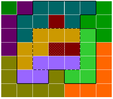
Figure 1. Grid and Social Neighbourhoods

2.5

Several different forms of Imitation are discussed. In Simple Imitation or SI, a weighted random choice is made between all Land Uses employed within the Social Neighbourhood of the Parcel in the preceding Year. The weights used are the number of Parcels in the Social Neighbourhood assigned to each Land Use in the most recent Year, i.e. the Land Use's popularity. Yield-based Imitation (YI) takes into account both the popularity of a particular Land Use in the most recent Year, and how successful it was, weighting the probability of choosing each Land Use by the total Yield for that Land Use across the Social Neighbourhood i.e. the sum of the Yields on all the Land Parcels on which that Land Use was employed. In Best-mean-weighted Imitation (BI), the random choice is weighted by the mean Yield of each Land Use on Parcels in the Social Neighbourhood (so only success, not popularity, counts).

2.6

These forms of imitation all calculate scores for Land Uses, then make a probabilistic choice between them using those scores as weights. An alternative is to choose only among those which score highest - so if one Land Use scores higher than any other, it will be chosen automatically, while if two or more have equal highest scores, each will have an equal probability of being chosen. We call the three corresponding imitation strategies Selective Simple Imitation (SSI), Selective Yield-based Imitation (SYI), and Selective Best-mean Imitation (SBI). We thus have six forms of Imitation to consider, in addition to Random Experimentation. Figure 2 and the accompanying table 1 give an example of Land Use selection by each of the six forms of Imitation.

2.7

In figure 2, Last Year's Land Uses and Yields for each Land Parcel are represented by letters and numbers respectively. Only those Land Parcels within the Social Neighbourhood of the central, stippled Parcel would be considered in deciding which Land Use to imitate (Land Uses and Yields of these Parcels are noted in white). Table 1 gives the number of Parcels, total Yield and mean Yield for each Land Use over those 28 Parcels. Land Use C is absent from the Social Neighbourhood, and so would not be considered. The row maxima (in bold italics) indicate which Land Use would be imitated when using each of the selective Algorithms (SSI: A, SYI: A or D with 0.5 probability each, SBI: E). To calculate the probability of imitating each Land Use with the proportional weighting Algorithms (SI, SYI, SBI), divide the number in the relevant cell by the number in the "Sum" column.

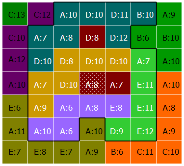
Figure 2. Calculation of Land Use to Imitate

Table 1: Calculation of Land Use to Imitate
Land Use	A	B	C	D	E	Sum
Number of Parcels (used in SI/SSI)	12	2	0	10	4	28
Total Yield (used in YI/SYI)	93	16	0	93	42	244
Mean Yield (used in BI/SBI)	7.75	8	N/A	9.3	10.25	35.3

2.8

Polhill, Gotts and Law (2001) and Gotts, Polhill and Adam (2003) found that a small admixture of Random Experimentation sometimes makes a big difference to simulations involving Algorithms otherwise depending wholly on Habit and Imitation. It can be either a small disadvantage or a small advantage to the Land Managers employing it, but if all Land Managers in a simulation rely wholly on Habit or Imitation, the number of Land Uses available declines, eventually leaving Land Managers no choice. Performance differences between Algorithms are then greatly diminished. Since our interest here is in the effects of different Aspiration Thresholds, and forms of Imitation, all the Selection Algorithms used employ Random Experimentation at least occasionally. "Habit-Random" (HR) Algorithms always use Random Experimentation if their Aspiration Threshold is not met. All other Subpopulations use it with a 1/16 probability when the Threshold is not met, but with 15/16 probability use one of the six forms of Imitation. Thus in addition to HR we have HRBI ("Habit-Random-Best-mean-Imitation), HRSBI, HRSI, HRSSI, HRYI and HRSYI Algorithms.

Simulation Environments

2.9

In all FEARLUS models used here, the Land Parcels form a 7 by 7 or 21 by 21 toroidal grid, which permits experiments involving relatively large numbers of runs, and avoids edge effects. The bitstrings defining Land Uses' preferred conditions always contain 16 bits. Environments differ in the division of these bits between Biophysical Characteristics (variable across space, but fixed over time) and External Conditions (uniform across space but usually variable over time). In new experiments reported here, the Break Even Threshold is always 8 (Gotts, Polhill and Law 2003, found that Environments with a Break Even Threshold lower or higher than half the maximum Yield reduce performance differences between Selection Algorithms), and the Land Parcel Price always 16.

2.10

The effect of using Land Parcel Biophysical Characteristics bits is that for any given Land Parcel, some Land Uses will generally have an advantage over others. The Biophysical Characteristics of Land Parcels may be either clumped or unclumped. In either case, each bit is initially set to 0 or 1 with equal probability and independently, for every Land Parcel. In the "clumping" process, carried out on each bit-position in turn during initialisation, adjacent Land Parcels are selected at random to swap non-matching bit-values, for as long as there is a swap which increases the number of neighbouring Land Parcels pairs that have the same value. In the Environments used here, either all Biophysical bits are clumped or all are unclumped; completely unclumped Environments are unrealistic, but variations in clumpiness certainly exist, and the inclusion of the unclumped Environments allows the effect of such variation to be investigated.

2.11

External Conditions may be fixed or variable, and if variable, either correlated or uncorrelated from Year to Year (in the former case, the Flip Probability used here is 1/8; in the latter, it must be 1/2). As we consider models with more Land Parcels, run for longer, FEARLUS models in which all External Conditions are variable approach a limit where all Land Uses give equal Yields, averaged over space and time. Allowing Fixed External Conditions means this is no longer so: each Fixed External Condition bit gives an advantage to those Land Uses which match it over those which do not, which operates on all Parcels and in all Years. Such bits represent factors which can be assumed constant over time and over a large region.

2.12

All Environments used except one can be described using the following syntax: S<m>{c,u}-T<n>{c,u}, where <m > and <n > stand for non-negative integers, "{" and "}" around a set of comma-delineated elements indicates that either one of this set, or nothing, can be expected, and "S" and "T" stand for "spatial" and "temporal" respectively. Thus "S12u-Tc4" indicates 12 unclumped Land Parcel Characteristic bits and 4 correlated External Conditions bits. These characteristics of an Environment are referred to as its Type. Zero-length bitstrings indicate no spatial — or no temporal — variation, so S0-T16c means no spatial variation and 16 bits of correlated temporal variation. Most of the experiments described here use one of the following eight Environment types: S0-T16c, S0-T16u, S16c-T0, S16u-T0, S8c-T8c, S8c-T8u, S8u-T8c, S8u-T8u.

2.13

Thus we use two spatially homogeneous but time-varying Environment types (with the variability either correlated or uncorrelated), two unvarying but spatially heterogeneous types (with the spatial variation clumped or unclumped), and four which vary over both space and time.

2.14

In S0-T16c Environments, Imitation should be very useful: without spatial variation, each Land Parcel will give the same Yield; and since temporal variation is correlated, what worked well last Year is likely to work well this Year. In S0-T16u Environments, by contrast, Random Experimentation should do at least as well as any form of Imitation, because all Land Uses will have the same expected Yield in every Year on every Parcel. In fact it does better than many others (Gotts, Polhill, Law and Izquierdo 2003): diversity gives some security against large losses once a Land Manager controls multiple Parcels.

2.15

In S16c-T0 and S16u-T0 Environments, there is no change from Year to Year, so a Land Use that returns at least the Manager's Threshold on a Land Parcel, will never be changed. Hence success should depend on the speed with which a Selection Algorithm finds such a Land Use, but also on just how rewarding the Land Use found is likely to be - as particularly profitable ones can compensate for losses elsewhere, and allow the Land Manager to expand their holding when the opportunity arises. Some kinds of Imitation at least should allow their users to take advantage of others' experience more effectively than Random Experimentation, but Imitators will only be able to exploit this advantage for a short time, so its benefits are likely to be less than in S0-T16c, where they can track change over time. Imitation should have more benefit in S16c-T0 than in S16u-T0, as nearby Parcels will on average be more similar. Of the other four Environment types we focus on (S8c-T8c, S8c-T8u, S8u-T8c and S8u-T8u), S8c-T8c should be intermediate between S0-T16c and S16c-T0. The other three could be expected to be less favourable to Imitation than S8c-T8c, with S8u-T8u being least favourable.

Simulation Experiments

2.16

Most of the FEARLUS experiments discussed here consist of multiple simulation runs, pitting two Subpopulations using different Selection Algorithms against each other in Contests to assess their success in specific types of Environment. Land Managers are equally likely to belong to either Subpopulation. At the start of each run, each Land Parcel is assigned to a different Land Manager. At the end (after 200 Years), Subpopulation success is assessed by counting the Parcels assigned to members of each. The runs in an experiment differ from only because a new seed is generated for each run. The binomial test is used to determine whether either Selection Algorithm has finished significantly more runs holding a majority of the Land Parcels than the other. For many of the Contest experiments reported, we made predictions of the results (based on the results of exploratory experiments, and our hypotheses about the mechanisms producing them). We report these predictions along with the results. The latter are taken to be significant when they reach the .01 level (1 tailed).

2.17

The remaining experiments use a single Subpopulation whose members vary in their Aspiration Threshold, the result of primary interest being the mean Aspiration Threshold at the end of the run.

Effects of Aspiration Thresholds

3.1

Experiments on HR Selection Algorithms (reported in Gotts, Polhill and Law 2003), indicated that the Aspiration Threshold makes a considerable difference to the performance of Subpopulations using these Algorithms, across a wide range of Environments with Land Use bitstrings of length 16, no fixed bits, and a Land Parcel Price of twice the Break Even Threshold (which varied between 4 and 12). The overall picture was complex, but the effects can be summarised as follows:

• The optimal Aspiration Threshold appeared never to exceed whichever is the greater of the Break Even Threshold, and 8 - the Yield that would be expected from a random choice of Land Use, henceforth Random Choice Expected Yield, (half the maximum Yield). Random Selection in these Environments has an expected Yield of 8, so if the current Yield is above 8, Random Selection can be expected to reduce it.
• However, if the Break Even Threshold was above 8, and inter-Year predictability was high, the optimal Aspiration Threshold did sometimes exceed 8. In such Environments, it may be worth experimenting, despite immediate expected losses, to find the Land Use best suited to a Land Parcel.
• In Environments with a Break Even Threshold of 8 and a lot of uncorrelated temporal variation in External Conditions, an Aspiration Threshold somewhat below 8 appeared optimal. Here, even a Land Use well suited to the Land Parcel will sometimes produce a loss; only a large loss is a good indication that an alternative should be tried.

3.2

Gotts, Polhill and Adam (2003) also reported experiments with HRSBI Land Managers, which indicated that in Environments with high inter-Year predictability and a Break Even Threshold equal to the Random Choice Expected Yield, the optimal Aspiration Threshold could exceed the Break Even Threshold. In a spatially heterogeneous FEARLUS Environment, Selective Best-mean Imitation could be risky, but in a spatially homogeneous one, switching to the Land Use with the highest mean Yield cannot give a lower expected Yield than sticking with the current one, unless Year y 's Yields are negatively correlated with those of Year y + 1. This implies that HRSBI could allow high Aspiration Thresholds to give good results in Environments with little or no spatial heterogeneity. Experiments setting H8RSBI (HRSBI with Aspiration Threshold 8) against H10RSBI in the eight Environment types defined above, and in both 7 by 7 and 21 by 21 Environments, showed that H10RSBI outperformed H8RSBI only in S0-T16c (in both 7 by 7 and 21 by 21), and in S8c-T8c (21 by 21 only). This result was reversed in S8c-T8u, S8u-T8u, S16c-T0 and S16u-T0 (in both 7 by 7 and 21 by 21 Environments). HRSBI stood out as a clear exception among the seven families of Selection Algorithms: in none of the other six did an Aspiration Threshold of 10 outperform one of 8 in any Environment type.

3.3

Contests between distinct Subpopulations are only one approach to investigating the effects of Aspiration Threshold (or anything else) on competitive performance. We have used one alternative to check the robustness of our findings on Aspiration Thresholds. In this approach, all Land Managers in the simulation run have the same Land Use Selection Algorithm, except for variation in the Aspiration Threshold. Whenever a Land Manager is created, its Aspiration Threshold is drawn from a prespecified distribution. Given repeated runs in a given Environment, an estimate of the mean Aspiration Threshold after a given period of time can be calculated, along with confidence intervals for this estimate. Since good performance by higher Aspiration Threshold Land Managers will push this value up, and success for lower Aspiration Threshold Managers will pull it down, the outcome provides a way of estimating optimal Aspiration Thresholds. Table 2 shows the results for the seven families of Algorithm (columns) and eight types of Environment (rows) tested. The prespecified statistical distribution from which Aspiration Thresholds are drawn was a uniform distribution with limits 3.5 and 12.5; hence a mean of 8.

3.4

Overall, the results are consistent with those of paired-Subpopulation experiments on Aspiration Thresholds, but bring out some points those experiments did not. In table 4 the figures in the cells are italicized if the 95% confidence interval for the value of the mean Aspiration Threshold lies wholly below 8, and bolded if it lies wholly above 8. It will be seen that in two Environment types (S8u-T8u and S16u-T0) the 95% confidence interval falls wholly below 8 for all Algorithms, although not by much. This suggests that in these Environments, it is advantageous to stay with a Land Use that just breaks even. The same is true in most Environment types for two families of Land Use Selection Algorithm: HR and HRSSI. Again, the deviation from the break-even value of 8 is small. For four families of Algorithm (HRYI, HRSYI, HRBI, HRSBI) the 95% confidence interval lies wholly above 8 in at least half the Environment types. Thus the results confirm that both Environment type and Algorithm family affect the relative advantages of different Aspiration Thresholds; but in most cases not by very much. HRBI and HRSBI are confirmed as unusual in favouring Aspiration Thresholds well above 8 (and in one Environment type, S0-T16c, above 9); although HRYI and HRSYI also favour Aspiration Thresholds above 8 (a result not found before), this was to a markedly lesser degree.

Table 2: Estimate and 95% confidence intervals [in brackets] for mean of Aspiration Thresholds across Land Parcels in FEARLUS 21 by 21 Environments. 60 runs of 200 simulation Years for each combination of Algorithm class (columns) and Environment type (rows)
	HR	HRSI	HRSSI	HRYI	HRSYI	HRBI	HRSBI
S0-T16c	7.956 [0.082]	8.481 [0.059]	7.951 [0.070]	8.840 [0.046]	8.236 [0.073]	9.103 [0.074]	9.089 [0.069]
S0-T16u	8.031 [0.051]	7.985 [0.043]	7.926 [0.051]	8.016 [0.057]	7.919 [0.062]	7.948 [0.099]	7.982 [0.091]
S8c-T8c	7.835 [0.057]	8.252 [0.045]	7.871 [0.055]	8.491 [0.046]	8.306 [0.053]	8.884 [0.036]	8.932 [0.040]
S8u-T8c	7.862 [0.055]	7.935 [0.053]	7.619 [0.061]	8.194 [0.058]	7.809 [0.063]	8.705 [0.044]	8.727 [0.043]
S8c-T8u	7.366 [0.043]	8.042 [0.046]	7.837 [0.061]	8.119 [0.042]	8.140 [0.053]	8.329 [0.057]	8.267 [0.071]
S8u-T8u	7.482 [0.040]	7.488 [0.041]	7.570 [0.057]	7.465 [0.041]	7.533 [0.063]	7.434 [0.062]	7.468 [0.064]
S16c-T0	7.735 [0.036]	8.006 [0.032]	7.974 [0.042]	8.129 [0.039]	8.213 [0.031]	8.354 [0.031]	8.394 [0.028]
S16u-T0	7.756 [0.029]	7.802 [0.034]	7.899 [0.033]	7.767 [0.035]	7.886 [0.036]	7.835 [0.031]	7.844 [0.032]

3.5

In conclusion, using a fixed Aspiration Threshold of 8 across Environment types and Selection Algorithm families is unlikely to distort comparisons between the latter.

When Imitating, Best-mean Imitation is Best

4.1

Moving on from the investigation of how Aspiration Thresholds affect performance across both Environment types and Selection Algorithm families, we turn to investigating competition between members of the different families. We focus again on the eight Environment types discussed above, making brief mention of others chosen to check the generality of the findings from them. We found clear differences between Environments: the result of Contests between a given pair of Algorithms can frequently be reversed by changing the pattern of spatio-temporal heterogeneity in the Environment; and in two cases by changing the Environment's size.

4.2

In all eight Environment types, we ran Contests between each pair from the Selection Algorithms H8R, H8RSI, H8RYI, H8RBI, H8RSSI, H8RSYI and H8RSBI. In the Environment type S0-T16c only, we ran Contests between each pair from these seven plus H10R, H10RSI, H10RYI, H10RBI, H10RSSI, H10RSYI and H10RSBI; this was done because the results reported above show that in this Environment type, H10RSBI does better than H8RSBI, and the mean Aspiration Threshold for HRSBI and a number of other Algorithm families rises well above 8 in the experiments with results shown in Table 2. The Contests involving Algorithms with Aspiration Threshold 10 are dealt with later in this section.

4.3

Tables 3-6 show the results of Contests between the seven Algorithms with Aspiration Threshold 8. Each table shows results for two of the eight Environment Types, and for Environments of two different sizes: 7 by 7 (120 runs per Contest), and 21 by 21 (60 runs per Contest). The figure on the left in each cell concerns the 7 by 7 Contest between a pair of Selection Algorithms in a specific type of Environment, the figure in parentheses on the right of the cell, the 21 by 21 Contest. In the upper-right half of each table, these figures give the number of runs ending with an advantage to the column Algorithm; in the lower-left half, the figures indicate the number of runs ending with an advantage to the row Algorithm. Figures in red indicate an advantage to the column Algorithm significant at the .01 level (two-tailed) in the upper-right half, to the row Algorithm at the same significance level in the lower-left half; those in blue, such an advantage for the other Algorithm. For example, the blue "18 (1)" toward the top left of Table 3 means that HRBI won only 18 out of 120 runs against HRSBI in the 7 by 7 Contest in S0-T16c, and only 1 out of 60 in the 21 by 21, and that these margins were significant at the .01 level (two-tailed). In S0-T16u, however, the corresponding figures for H8RBI were 57 and 40, neither significant at the chosen level. These arrangements thus facilitate comparison of results in Environments of different sizes, and of results in the types of Environment in the two halves of the table. Figure 3 shows the results involving H8RSBI in graphical form. The coloured bars show the number of runs won by H8RSBI in the 7 by 7 Environments (read off the bottom scale of each subfigure). Where the proportion of wins in the corresponding 21 by 21 Environment for the same pairing of Selection Algorithms is different, this is shown by an additional line across the coloured bar, or an uncoloured extension of the bar (number of wins for H8RSBI being read off the top scale).

4.4

The most obvious outcome of these experiments is the success of the H8RSBI Selection Algorithm: across all Environment types except S0-T16u, and across both 7 by 7 and 21 by 21 Environments, it outperforms the four Algorithms that use Simple or Yield-based Imitation (H8RSI, H8RSSI, H8RYI and H8RSYI). It also outperforms both H8RBI and H8R in S0-T16c, S8c-T8c, S8u-T8c, S8c-T8u and S16c-T0. It is never outperformed by H8RBI; and is outperformed by H8R only in S0-T16u - the Environment type where maximizing Land Use diversity should be most advantageous.

Table 3: Outcomes of some Selection Algorithm Contests in spatially homogeneous, temporally variable Environments (upper-right in both : S0-T16c; lower-left: S0-T16u)
	H8RSBI	H8RBI	H8RSYI	H8RYI	H8RSSI	H8RSI	H8R
H8RSBI	—	18 (1)	16 (1)	8 (0)	7 (0)	6 (1)	8 (1)
H8RBI	57 (40)	—	41 (14)	56 (21)	12 (1)	32 (8)	35 (3)
H8RSYI	65 (25)	50 (27)	—	90 (54)	25 (2)	71 (36)	54 (25)
H8RYI	62 (23)	59 (29)	59 (37)	—	9 (0)	32 (6)	39 (8)
H8RSSI	49 (23)	45 (33)	52 (29)	58 (32)	—	107 (58)	94 (57)
H8RSI	59 (30)	62 (28)	65 (32)	58 (29)	70 (27)	—	63 (22)
H8R	70 (42)	74 (33)	77 (31)	70 (39)	82 (38)	67 (39)	—

Table 4: Outcomes of some Selection Algorithm Contests in spatially variable, temporally unchanging Environments (upper-right: S16c-T0, lower-left: S16u-T0)
	H8RSBI	H8RBI	H8RSYI	H8RYI	H8RSSI	H8RSI	H8R
H8RSBI	—	29 (2)	34 (1)	36 (0)	19 (0)	40 (1)	29 (1)
H8RBI	54 (24)	—	59 (23)	49 (27)	30 (4)	56 (15)	49 (20)
H8RSYI	30 (2)	46 (7)	—	69 (38)	42 (8)	61 (18)	61 (28)
H8RYI	44 (22)	54 (23)	79 (53)	—	29 (5)	65 (26)	56 (22)
H8RSSI	34 (1)	34 (2)	55 (22)	35 (3)	—	80 (49)	83 (47)
H8RSI	58 (17)	61 (15)	81 (53)	56 (25)	85 (58)	—	64 (29)
H8R	57 (29)	75 (33)	80 (56)	66 (44)	90 (60)	68 (46)	—

Table 5: Outcomes of some Selection Algorithm Contests in spatially variable, temporally variable but auto-correlated Environments (upper-right: S8c-T8c, lower-left: S8u-T8c)
	H8RSBI	H8RBI	H8RSYI	H8RYI	H8RSSI	H8RSI	H8R
H8RSBI	—	14 (0)	12 (0)	21 (0)	5 (0)	18 (0)	11 (0)
H8RBI	35 (0)	—	41 (20)	57 (25)	13 (0)	48 (15)	40 (6)
H8RSYI	7 (0)	17 (0)	—	83 (49)	37 (2)	83 (38)	79 (16)
H8RYI	23 (1)	37 (14)	101 (60)	—	11 (0)	42 (17)	47 (6)
H8RSSI	5 (0)	7 (0)	43 (12)	10 (0)	—	102 (59)	87 (48)
H8RSI	20 (1)	44 (10)	97 (59)	45 (18)	101 (60)	—	59 (12)
H8R	22 (0)	65 (28)	104 (60)	56 (43)	114 (60)	79 (48)	—

Table 6: Outcomes of some Selection Algorithm Contests in spatially variable, temporally variable and uncorrelated Environments (upper-right: S8c-T8u, lower-left: S8u-T8u
	H8RSBI	H8RBI	H8RSYI	H8RYI	H8RSSI	H8RSI	H8R
H8RSBI	—	32 (3)	24 (3)	28 (5)	18 (0)	26 (3)	19 (0)
H8RBI	61 (29)	—	45 (29)	62 (35)	22 (6)	56 (25)	43 (2)
H8RSYI	21 (0)	15 (0)	—	88 (42)	39 (4)	75 (30)	67 (1)
H8RYI	37 (12)	49 (13)	99 (59)	—	15 (3)	39 (15)	42 (1)
H8RSSI	21 (0)	17 (0)	63 (20)	25 (0)	—	88 (60)	81 (11)
H8RSI	38 (12)	45 (13)	98 (60)	60 (26)	100 (59)	—	48 (4)
H8R	54 (33)	65 (42)	102 (60)	60 (45)	103 (60)	74 (48)	—

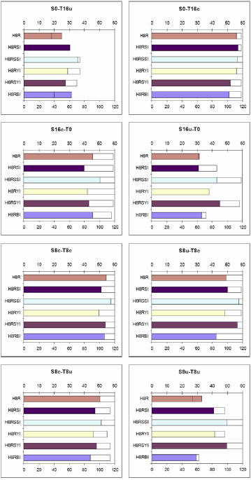
Figure 3. Outcomes of Contests from Table 3 involving H8RSBI

4.5

In S0-T16c Environments, a Land Use's mean Yield in the Neighbourhood is a better guide than total Yield across the Neighbourhood, and this in turn is better than the number of Parcels where it is used. Choosing only among the highest scorers works well only if the mean Yield is used; otherwise, weighting proportional to the scores does better. Clearly, with a good enough scoring system, choosing only from the very best scorers should work well; but why is it a disadvantage with one that is less good, but still better than random, as appears to be the case when we compare HRYI with HRSYI? The likely answer is the advantage that Land Uses diversity has both for individual Land Managers and for Subpopulations (Gotts, Polhill, Law and Izquierdo 2003).

4.6

In S0-T16u Environments, by contrast (where Year to Year change is wholly unpredictable), the expected advantage for Land Use diversity appeared, with H8R outperforming the three "Selective" Algorithms: H8RSBI, H8RSYI and H8RSSI - which are those that should produce least diversity (and no other significant results).

4.7

With the exception of S0-T16u, the order of the Imitation Algorithms is pretty consistent: H8RSBI at the top, then H8RBI and H8RYI, then H8RSI and H8RSYI, finally H8RSSI. The very poor performance of H8RSSI is presumably due to Land Managers using it getting trapped in a single Land Use, even when conditions change: it would be very difficult for a Population consisting entirely of HRSSI Managers to escape from a near-monoculture once formed, despite the component of Random Experimentation. In all Environment types except S0-T16u, H8RSI outperformed H8RSSI; and in all except S0-T16u and S16c-T0 H8RYI outperformed H8RSYI, confirming that if the scoring criterion used in deciding what to imitate is not particularly good, a weighted choice is better than selecting from the highest scorers only. Furthermore, H8R outperformed H8RSSI in all the four Environments, and H8RSYI in all but the S8c-T8u case, confirming that Imitation can give worse outcomes than Random Experimentation.

4.8

The position of HR relative to this hierarchy, however, changes substantially, although it is always above H8RSSI. It is highest in S0-T16u (as expected), then S8u-T8u and S16u-T0, S8c-T8u, S16c-T0, S8u-T8c, S8c-T8c and S0-T16c. Note that among the four Environment Types with both spatial and temporal variation, the spatially clumped Environments (S8c-T8c and S8c-T8u), in which nearby Parcel pairs are likely to resemble each other more than distant ones, were more favourable to Imitative Selection Algorithms than the other two. Temporal correlation also appears to improve the relative performance of Imitation relative to Random Experimentation, but to a lesser extent.

4.9

Reversals of competitive advantage between the types of Environment differing only in the correlated or uncorrelated nature of either spatial or temporal variation (i.e., between the pairs of Environment types in each of tables 3-6) occur, with one exception, only in Contests between H8R and others, adding to the evidence that the competitive relationships between forms of Imitation are considerably more robust under changes of Environment than those between Imitation and Random Experimentation.

4.10

The only reversals of competitive advantage between large and small Environments of the same type occur in the S8c-T8c H8R/H8RSYI Contest and the S8c-T8u H8R/H8RSSI Contest, where the Imitative Algorithm outperforms H8R in large Environments, but is outperformed in small ones. (More generally and with few exceptions, small-Environment Contests are less one-sided than the corresponding large-Environment ones.) These reversals hint that Imitation works better in the larger Environments, at least where there is clustered spatial variation, perhaps because in these Environments, there are likely to be at least some sizeable patches where there is little spatial variation.

4.11

The Contests recorded in the upper-right of table 3 are a subset of those undertaken in S0-T16c Environments. The results of corresponding Contests among Selection Algorithms with Aspiration Threshold 10 are shown in table 7. There are few large differences from table 3; most noticeable is that H10R does less well than did H8R, while H10RBI fails to outperform H10RSYI as H8RBI did H8RSYI. In the 7 by 7 Environments, each of the 14 Algorithms was in fact matched against each of the others and a fairly clear pattern emerged: the most important difference was between Families of Algorithms, not Aspiration Thresholds: HRSBI performed best; then HRBI and HRYI; then HRSI, HRSYI and HR; and finally HRSSI. At the top of the order of Families, Aspiration Threshold 10 was better than Threshold 8, in the middle there was little to choose between these Aspiration Thresholds, and at the bottom Threshold 10 performed worse. It makes sense that the better the procedure used when the Aspiration Threshold is not met, the higher the optimal Threshold tends to be, as that procedure will be used more when the Threshold is higher.

Table 7: Outcome of some Selection Algorithm Contests between Algorithms with Aspiration Threshold 10, in spatially homogeneous, temporally variable but correlated Environments
	H10RSBI	H10RBI	H10RSYI	H10RYI	H10RSSI	H10RSI	H10R
H10RSBI	—	12 (1)	19 (3)	17 (1)	7 (0)	8 (1)	0 (0)
H10RBI		—	58 (30)	71 (29)	14 (7)	39 (8)	9 (0)
H10RSYI			—	86 (46)	35 (6)	68 31	31 (9)
H10RYI				—	9 (2)	26 (3)	13 (1)
H10RSSI					—	112 (59)	92 (50)
H10RSI						—	31 (10)
H10R							—

4.12

So far, we have not seen any Environments in which HRSBI is definitely inferior to any of the other Imitative Selection algorithms investigated. However, there are indeed such Environments, specifically those which are highly unpredictable Year to Year, but still give the Land Manager something useful to learn about what Land Uses to employ where (S0-T16u Environments are maximally unpredictable among Environments with 16 bits of spatio-temporal variation, but all Land Uses have the same expected Yield on all Land Parcels). Specifically, we looked at S1u-T15u Environments (one bit of unclumped spatial variation, 15 of uncorrelated temporal variation). The advantage for an Aspiration Threshold below the Break Even Threshold (specifically, one of 6 compared to a Break Even Threshold of 8), found for the HR, HYI and HRYI Families of Algorithms by Gotts, Polhill, Law and Izquierdo (2003), also applied to the HRBI and HRSBI Families. We also confirmed that in S1u-T15u Environments, the Aspiration Threshold used had more influence than the procedure adopted if that Threshold was not reached.

4.13

We therefore looked at Contests between Subpopulations using pairs of Algorithms with Aspiration Threshold 6, running Contests between all pairs of such Algorithms in 7 by 7 Environments. The main points to note are:

• HR did well: in fact, H6R easily outperformed all the other Algorithms except H6RBI (against which it had a non-significant advantage).
• H6RBI clearly outperformed all the other imitative Algorithms.
• H6RSBI clearly outperformed the remaining four Algorithms, so Best-mean Imitation does better than Simple or Yield-based Imitation, as in all other Environment types tried other than the wholly unpredictable S0-T16u.

4.14

HRBI (and to a lesser extent HRSBI) may simply be less disadvantaged than other imitative Families, because Best-mean Imitation, unlike Simple and Yield-based Imitation, does not tend to copy the Land Uses which are currently most common on nearby Parcels, which is likely to reduce diversity.

4.15

Finally, we looked at a type of spatially homogeneous Environment in which, unlike those considered so far, some Land Uses gave higher expected Yields than others over time. The S0-T8f8u Environment type has eight bits of temporally uncorrelated variation in External Conditions, while another eight bits do not vary at all. The effect is that when Land Uses are assigned bitstrings at random, some Land Uses are likely to match these fixed External Conditions better than others. However, which Land Uses are objectively best will be partially obscured by the "noise" of the eight bits of uncorrelated variation. HRSBI was, as often, the most successful Family (and H10RSBI outperformed H8RSBI), but, in contrast to all the standard Environment types, HRSYI (Habit/Random/Selective-Yield-based-Imitation) outperformed HRYI (Habit/Random/Yield-based Imitation). In this type of Environment, then, a criterion of total Yield appears good enough to make choosing from among the best only, superior to choosing by proportional weighting - although still inferior to mean Yield. We hypothesise that because some Land Uses generally have higher expected Yields than others over the long term, the degree of "inertia" which Yield-based Imitation involves (tending to go on doing what most of your Neighbours have done) is less harmful than in the eight standard Environments. This interpretation is supported by the fact that the algorithms involving Simple Imitation outcompeted H8R - although losing to the other Imitative Algorithms with Aspiration Threshold 8 - showing that even the greater degree of inertia brought about by Simple Imitation is better than Random Experimentation in this type of Environment.

Discussion

5.1

The main conclusion of the work reported is that Best-mean Imitation is superior to Simple or Yield-based Imitation across a wide range of FEARLUS Environments; and that Selective Best-mean Imitation (choosing from among the best only) is generally better than using proportional weighting. This yields the prediction that when imitating neighbours, farmers will do better to adopt the currently best-performing land use in their neighbourhood rather than the most popular, or that producing the greatest total return across the neighbourhood - and, given the simplicity of the procedure, that when imitating they will actually do this or something similar.

5.2

Further possible lessons from the simulations reported can be summarised as follows:

1. The optimum aspiration threshold appears to depend primarily on the predictability of returns from alternative courses of action over time: the more unpredictable the world is, the lower the threshold, so that in some cases it should be set below what is needed to survive indefinitely.
2. In highly unpredictable environments, experimentation is at least as good as any form of imitation, when the aspiration threshold is not met.
3. In all but the most unpredictable environments, however, some form of imitation should outperform random experimentation; experiment only if no-one else is doing so. This advice, and the results behind it, suggest the existence of a social dilemma - a situation in which each of a group of interacting agents faces a choice between "selfish" and "cooperative" actions (experimenting at least occasionally being the cooperative choice); each will profit individually from the selfish choice (whatever others do); but all will be better off if all act cooperatively. However, the dilemma here may not be particularly sharp: only a little experimentation is required to avoid a decline into monoculture, so successful land managers might well be able to bear the costs.
4. Given a particular scoring criterion for alternative courses of action in any context, whether selection should be made from among the highest-scoring options only, or on some broader basis such as proportional weighting, depends on how good the criterion is. With a good enough criterion, selection from among the highest-scoring options only is superior to proportional weighting. This is particularly interesting because many of the key results of evolutionary game theory (Taylor and Jonker 1978; Bendor and Swistak 1997; Hofbauer and Sigmund 1998) depend on the assumption that any strategy which scores above the population mean will increase in frequency, even if there are superior strategies in the population. The assumption may be justified for biological evolution, but when agents learn from each other it would not in general hold if strategy-learning takes place by Selective Best-mean Imitation.

5.3

Work on imitation within FEARLUS in the context needs to be placed in the context of the most relevant studies in three areas:

• research on the adoption, or spread, of agricultural innovations,
• imitation within agent-based models of rural land use, and more briefly,
• work on imitation in spatial games.

5.4

Research on the adoption of agricultural innovations goes back to Ryan and Gross (1943). Only recently, however, have panel studies (Besley and Case 1994; Foster and Rosenzweig 1995; Pomp and Burger 1995) and anthropological/ethnographic studies (Letenyei 2001; Chiffoleau 2005) provided some detail concerning micro-level processes, confirming that farmers are influenced toward adopting new land uses or techniques by the example of other farmers they know.

5.5

There are few studies of the spatial characteristics of innovation diffusion, but most of the exceptions indicate that imitation of neighbours is indeed important. Ryan and Gross (1943), studying the diffusion of hybrid seed corn in Iowa, found that "Commercial channels, especially salesmen, were most important as original sources of knowledge, while neighbours were most important as influences leading to acceptance." Hägerstrand ( 1967) found that innovation spread from a few focal points, although not necessarily from farm to contiguous farm. Case (1992) found "strong neighbourhood effects" in the adoption of new farming technologies in Indonesia. Foster and Rosensweig ( 1995) found that farmers adopting HYV (high-yielding variety) wheat and rice benefited (in terms of productivity) from having neighbours who had already done so - confirming that they were learning about techniques from their neighbours rather than simply learning about new varieties' potential profitability. Rich farmers tended to adopt earlier, and poor farmers with richer neighbours possibly tended to delay their own adoption of new varieties, "free-riding" on the risk taken by those neighbours. Thus there is indirect evidence that innovation has significant costs, but for wealthier farmers, the potential longer-term gains may outweigh the risk of short-term losses. This suggests that if FEARLUS Land Managers were allowed to learn by trial and error how willing they should be to experiment, this willingness should come to correlate with wealth.

5.6

Schmidt and Rounsevell (2006) found that imitation leaves little noticeable trace on landscape pattern in a case study in central Belgium. Specifically, neighbouring parcels cultivated by farmers living in close proximity are "only slightly more similar" than neighbouring parcels cultivated by farmers living further from each other. The authors call into question the study of imitation in agent-based models of land use change. However, it is not clear how broadly generalizable this result is, as they admit: one might expect to find the clearest evidence of imitation of neighbours in situations of rapid change, whether involving completely novel innovations or the tracking of exogenous changes in profitability - and to determine whether rapid change is occurring, longitudinal studies are required. Moreover, if the choice of targets for imitation in the real world approximates to the Social Neighbourhood in FEARLUS, there is no reason to expect any effect of the distance between farmers' homes, once they share a parcel boundary: specifically, in the work reported above, FEARLUS Land Managers take equal account of all the Land Parcels owned by those with whom they share any parcel boundary (even a single point). The rationale for this is that being able to see something of the results a neighbour is getting on a regular basis will greatly increase the salience of that neighbour's successes and failures; a better test of the FEARLUS approach would be to examine whether, among pairs of land parcels at equal distances cultivated by different farmers, there is more land use similarity between pairs where the farmers cultivating them share a parcel boundary.

5.7

Turning to agent-based models of land use change, a number have modelled imitation, but FEARLUS appears to be the only one for which systematic performance comparisons between agents making use of imitation to different extents, and of different kinds, has been undertaken. Nonetheless, some comparisons may be useful.

5.8

Hägerstrand (1967) developed a series of simple simulation models (apparently without use of a computer, but employing tables of random numbers) attempting to reproduce the qualitative spatial features of innovation diffusion, described as follows (pp. 133-134):

• Stage 1. Local concentrations of initial acceptances (initial agglomerations).
• Stage 2. Radial dissemination outward from the initial agglomerations is accompanied by the rise of secondary agglomerations, while those original centres simultaneously continue to condense.
• Stage 3. The growth ceases (saturation phase).

5.9

A model in which the population falls into a number of "resistance classes", defined by the number of neighbours who must inform the individual they have adopted it before the individual themselves adopts, reproduced the qualitative features of the three-stage process above. This kind of adoption threshold is distinct from any of the selection criteria used with FEARLUS, but closer to Simple Imitation than to the Yield-based or Best-mean varieties, in that only the number of neighbours taking a particular course of action is considered.

5.10

Lansing and Kremer's model of a Balinese agricultural socio-ecosystem (Lansing and Kremer 1994; Lansing 2000) concerns the choice between a finite set of mutually exclusive alternatives, in this case cropping patterns in rain-irrigated rice-growing. The model uses something distinct from any of the approaches so far used with FEARLUS, although most similar to Selective Best-mean Imitation: the agents (farmers' cooperatives called subaks) copy the cropping pattern of their most successful neighbour; in FEARLUS Selective Best-mean Imitation, a single very good result could be outweighed by a number of poor ones. Also, a FEARLUS agent may have multiple choices to make (one per Land Parcel), and takes account of what has happened on individual Land Parcels, rather than on the land managed by each agent considered as a whole. Furthermore, the choices made by the subaks interact directly in a way that has no parallel in the FEARLUS models discussed here. Starting subaks with randomly assigned schedules, and allowing them to copy more successful neighbours, gave rise to spatio-temporal patterns of cropping qualitatively similar to those observed. It would be interesting to discover whether different forms of imitation, which could be modelled on the alternatives examined for FEARLUS here, would preserve this result, and to the extent each did so, whether it would alter the speed at which the system evolved (Janssen, 2007, shows that at least one way of changing both neighbourhood and imitation criterion together does alter the outcome). Conversely, FEARLUS experiments could be conducted using the "imitate the best" approach (at either Parcel or Manager level).

5.11

The "Consumat" approach to modelling decision-making (Janssen and Jager 1999; Jager et al 2000) has been applied in a spatially-explicit model of land use selection (Dung et al 2005). Agents have four different ways of making decisions, depending on levels of "satisfaction" (with the outcome of recent behaviour) and "uncertainty" (regarding the outcomes of behaviour, assessed by comparing expected and actual recent outcomes). If "satisfied" and "certain" they repeat previous behaviour; if "satisfied" and "uncertain" they imitate another agent's recent behaviour; if "unsatisfied" and "certain" they "deliberate" (use "reasoned individual processing" to assess expected outcomes); if "unsatisfied" and "uncertain" they use "social comparison" - observing what another agent has done, then calculating expected outcomes for that behaviour and their own previous behaviour, selecting whichever gives the higher expectation. In the model of Dung et al (2005), imitation and social comparison are based on the most popular choice among a set of agents (among three alternatives - rice growing, shrimp farming, or a mixture of the two). In every run, each agent was randomly assigned an individual satisfaction threshold and uncertainty threshold from the same distribution: there was no exploration of the results of changing these thresholds (altering the proportion of each behaviour), or of the relative performance of agents with different thresholds within a single simulation, although the development of economic inequality was one of the foci of the research.

5.12

There are some interesting points of comparison and contrast between this study and results from FEARLUS. The FEARLUS agents discussed here have a satisfaction threshold, like Consumat agents, but do not have an uncertainty threshold. When satisfaction (with regard to a specific Land Parcel) is above this threshold, the agent always repeats its previous action, in contrast to consumat agents, which will imitate the agent with which it has most recently compared itself when uncertainty is high, and repeat only when it is low. The association of social information processing with high uncertainty (whether satisfaction is high or low) is justified by Janssen and Jager (1999) by reference to Festinger's social comparison theory (Festinger 1954) which states (Janssen and Jager 1999, section 3.6) that:

"the drive to compare one's opinions and abilities with that of others is larger, the more uncertain one is regarding one's own opinions and abilities."

However, FEARLUS results reported here indicate that as Year-to-Year uncertainty increases (this is uncertainty inherent in the environment rather than measured by the individual agent from the accuracy of their predictions, but increasing inherent environmental uncertainty would make such predictions less accurate), repetition becomes increasingly favoured over Imitation of any kind, and the latter also becomes less favoured relative to Random Experimentation (probably because the rewards of Imitation fall, while those of diversity, which Random Experimentation tends to increase, do not). The results reported in Polhill, Gotts and Law (2001) also indicate that greater Year-to-Year uncertainty favours Selection Algorithms based on the long-term expected mean performance on specific Land Parcels at the expense of Imitative Selection Algorithms. In at least some kinds of decision-making, then, people behaving as Festinger and the consumat approach predict would lose out to those behaving differently. They may behave in such a manner, but when comparably simple alternatives would do better, it does seem likely selective pressures would lead to their adoption. How people actually change their tendency to imitative behaviour as environmental uncertainty increases would seem to be discoverable by laboratory experiment, but we have found no directly relevant studies.

5.13

There is extensive research on "spatial games", in which multiple players are embedded within a grid and play simple games such as the "Prisoner's Dilemma" against their neighbours. Each cell in the grid is initially assigned a strategy (drawn from some predefined strategy space), then one or more rounds of "play" between neighbours alternate with a strategy-updating process, interpreted either as reproduction, or as learning by imitation. Often (e.g. Nowak and Sigmund 1993; Grim 1996; Killingback et al 1999; Eguíluz, Zimmermann and Cela-Conde 2005), this uses "imitate the best" - the highest-scoring neighbour is copied. Other studies of imitation in simple spatial games use selective best-mean imitation (Eshel Samuelson and Shaked 1998; Eshel et al 2000; Noailly, Withagen and van den Bergh 2005); comparison with a random neighbour, with a probabilistic switch of strategy if the neighbour has done better (Kirchkamp 2000) - functionally similar to Simple Imitation; or comparison with the scores of each neighbour, with the strategy of a higher-neighbour being adopted with probability proportional to the difference in scores (Brandt, Hauert and Sigmund 2003).

5.14

Only a few such studies examine whether using different forms of imitation produces different outcomes. Cohen et al (1999) used three different imitation processes, along with a number of different strategy spaces for the game used - the iterated Prisoner's Dilemma - and different ways of defining a network of interaction, including a conventional two-dimensional grid. The three imitation processes were imitation of the highest-scoring neighbour without error (Imit), imitation (with errors) of the highest-scoring neighbour (BMGA), and imitation (with errors) of a random neighbour, if it had done better than the imitating agent (1FGA). These interacted with the strategy space and the form of network used in complex ways. Janssen (2000), by contrast (using the simple Prisoner's Dilemma), found no qualitative difference in results depending on whether imitate the best, or selective best-mean imitation was used. Yoon (2005), replicated the study of Eshel, Samuelson and Shaked (1998) on simple agents arranged in a circle, acting either altruistically or egoistically toward their neighbours, and then updating their choice of action by imitating successful neighbours - but substituted imitate the best for selective best-mean imitation. This drastically altered the dynamics of the situation, leading to a consistent fall in the frequency of cooperative behaviour in place of the rise found in the original study.

5.15

To summarise, much of the work reviewed here makes use of a particular form of imitation without consideration of the alternatives, although the FEARLUS experiments described, Janssen (2007) and some of the studies of simple spatial games mentioned show that different approaches to the question of when and how to imitate neighbours can make a profound difference. Conversely, non-FEARLUS work both suggests additional alternatives not yet tried within FEARLUS (such as "imitate the best"); and to differences between the adoption of truly novel land uses or land management practices on the one hand, and tracking potentially reversible changes in relative returns from different land uses on the other. FEARLUS has not yet been used to model the former, but there is no reason this should not be done. More difficult would be to adapt FEARLUS to model the often complex interactions between different innovations revealed in empirical work on innovation adoption, and the ability to profit from neighbours' experience of the techniques required to make a potential innovation successful suggested by work such as that of Foster and Rosensweig (1995).

5.16

Future FEARLUS work on imitation could reasonably drop these less successful forms of Imitation, and concentrate on the trade-off between selecting the most profitable Land Uses using Best-mean Imitation, and maintaining Land Use diversity. In the same way as the work shown in table 2 drew the Aspiration Threshold for each Land Manager from a continuous distribution, the probability a dissatisfied Land Manager uses Selective Best-mean Imitation rather than Random Experimentation could be set in the same way. This probability, and the Aspiration Threshold, could also be varied for individual Land Managers to allow trial-and-error learning; but it is not feasible that a farmer could observe and imitate these features of neighbours' decision processes, or inherit them. There remains plenty of mileage in extending FEARLUS modelling studies of imitation, but at some stage, a change from the representation of "Land Uses" as unitary packages, to more articulated representations of land management options, will be required.

Acknowledgements

We gratefully acknowledge statistical and mathematical advice from Mark Brewer of Biomathematics and Statistics Scotland. Any errors remain our responsibility. This work was funded by the Scottish Government Rural and Environment Research and Analysis Directorate, whom we thank.

Notes

¹ Terms for FEARLUS model constructs are given upper-case initial letters, and italicised on first use.

² The experiments newly reported here used FEARLUS versions 0-5-1-4, 0-5-1-5 (which differ only slightly) and 0-6-8-2. Versions 0-5-1-5 and 0-6-8-2, and relevant parameter files and scripts, are available from the authors.

References

ABADI GHADIM, A.K. and Pannell, D.J. (1999) A conceptual framework of adoption of an agricultural innovation. Agricultural Economics 21:145-154.

BENDOR, J. and Swistak, P. (1997) The evolutionary stability of cooperation. American Political Science Review 91(2):290-307.

BESLEY, T. and Case, A. (1994) Diffusion as a Learning Process: Evidence from HYV Cotton. Discussion Paper #174, Research Program in Development Studies, Center of International Studies, Woodrow Wilson School of Public and International Affairs, Princeton University.

BRANDT, H., Hauert, C. and Sigmund, K. (2003). Punishment and reputation in spatial public goods games. Proceedings of the Royal Society of London B 270:1099-1104.

CASE, A. (1992) Neighborhood influence and technological change. Regional Science and Urban Economics 22(3):491-508.

CHIFFOLEAU, Y. (2005) Learning about innovation through networks: the development of environment-friendly viticulture. Technovation 25:1193-1204.

COHEN, M. D., Riolo, R. L.& Axelrod, R. (1999). The Emergence of Social Organization in the Prisoner's Dilemma: How Context-Preservation and other Factors Promote Cooperation. Working Paper 99-01-002, Santa Fe Institute.

CRAMB, R.A., Garcia, J.N.M., Gerrits, R.V. and Saguiguit, G.C. (1999) Smallholder adoption of soil conservation techniques: evidence from upland projects in the Philippines. Land Degradation and Development 10:405-423.

DUNG, L.C., Vinh, N.N.G.V., Tuan, L.A. and Bousquet, F. (2005) Economic differentiation of rice and shrimp farming systems and riskiness: a case of Bac Lieu, Mekong Delta, Vietnam, in : F. Bousquet, F., Trebuil, G. and Hardy, B. Companion Modeling and Multi-agent Systems for Integrated Natural Resource Management in Asia. Metro Manila, International Rice Research Institute, p. 211-235.

EGUÍLEZ, V.M., Zimmermann, M.G., Cela-Conde, C.J. and San Miguel, M. (2005) Cooperation and the Emergence of Role Differentiation in the Dynamics of Social Networks. American Journal of Sociology 110(4): 977-1008.

ESHEL, I., Herreiner, D. K., Samuelson, L., Sansone, E. & Shaked, A. (2000). Cooperation, Mimesis and Local Interaction Sociological Methods and Research 28(3): 341-364.

ESHEL, I., Samuelson, L. & Shaked, A. (1998). Altruists, Egoists and Hooligans in a Local Interaction Model. American Economic Review 88(1): 157-179.

FEDER, G. and Slade, R. (1984) The Acquisition of Information and the Adoption of New Technology. American Journal of Agricultural Economics 66(3):312-320.

FESTINGER, L. (1954). A theory of social comparision processes. Human Relations 7:117-140.

FOSTER, A. D. and Rosenzweig, M.R. (1995) Learning by Doing and Learning from Others: Human Capital and Technological Change in Agriculture. Journal of Political Economy 103(6):1176-1209

FUJISAKA, S. (1994) Learning from six reasons why farmers do not adopt innovations intended to improve sustainability of upland agriculture. Agricultural Systems 46:409-425.

GOTTS, N.M., Polhill, J.G. and Law, A.N.R. (2003) Aspiration levels in a land use simulation. Cybernetics and Systems 34(8):663-683.

GOTTS, N.M., Polhill, J.G. and Adam, W. J. (2003) Simulation and Analysis in Agent-Based Modelling of Land Use Change. Proceedings, First conference of the European Social Simulation Association September 18-21, Groningen, The Netherlands, http://www.uni-koblenz.de/~essa/ESSA2003/.

GOTTS, N.M., Polhill, J.G., Law, A.N.R. and Izquierdo, L.R. (2003) Dynamics of imitation in a land use simulation. In Dautenhahn, K. and Nehaniv, C.L. (Eds.) Proceedings of the AISB '03 Second International Symposium on Imitation in Animals and Artifacts, 7-11 April, The University of Wales, Aberystwyth, The Society for the Study of Artificial Intelligence and Simulation of Behavious (SSAISB), pp.39-46. Also available online at http://www.macaulay.ac.uk/fearlus/FEARLUS-publications.html.

GRIM, P. (1996). Spatialization and Greater Generosity in the Stochastic Prisoner's Dilemma. BioSystems 37: 3-17.

HÄGERSTRAND, T. (1967) Innovation Diffusion as a Spatial Process, translated and with a postscript by Pred, A., translation with the assistance of Haag, G. University of Chicago Press, Chicago.

HIEBERT, L.D. (1974) Risk, Learning, and the Adoption of Fertilizer Responsive Seed Varieties. American Journal of Agricultural Economics 56:764-768.

HOFBAUER, J. and Sigmund, K. (1998) Evolutionary Games and Population Dynamics. Cambridge, UK, Cambridge University Press.

JAGER, W., Janssen, M.A., De Vries, H.J.M., De Greef, J. and Vlek, C.A.J. (2000) Behaviour in Commons Dilemmas: Homo economicus and Homo psychologicus in an Ecological-Economic Model. Ecological Economics 35:357-379.

JANSSEN, M.A. and Jager, W. (1999) An Integrated Approach to Simulating Behavioural Processes: A Case Study of the Lock-In of Consumption Patterns. Journal of Artificial Societies and Social Simulation 2(2) https://www.jasss.org/2/2/2.html.

JANSSEN, M.C.W. (2000) Imitation of Cooperation in Prisoner's Dilemma Games with Some Local Interaction. Tinbergen Institute Discussion Paper TI 2000-019/1

JANSSEN, M.C.W. (2007) Coordination in Irrigation Systems: An Analysis of the Lansing-Kremer model of Bali. Agricultural Systems 93:170-190.

KILLINGBACK, T., Doebeli, M. & Knowlton, N. (1999). Variable Investment, the Continuous Prisoner's Dilemma, and the Origin of Cooperation. Proceedings of the Royal Society of London B 266:1723-1728.

KIRCHKAMP, O. (2000). Evolution of Learning Rules in Space. In Suleiman, R., Troitzsch, K.G. and Gilbert, G.N. (Eds.) Tools and Techniques for Social Science Simulation, Chapter 10, pp.179-195. Berlin, Physica-Verlag.

LANSING, J. S. (2000) Anti-Chaos, Common Property and the Emergence of Cooperation. In Kohler, T.A. and Gumerman, G.J. (Eds.) Dynamics in Human and Primate Societies, pp.207-223. Santa Fe Institute Studies in the Sciences of Complexity. Oxford University Press, Oxford.

LANSING, J. S. and Kremer, J.N. (1994) Emergent properties of Balinese water temple networks: coadaptation on a rugged fitness landscape. Artificial Life III. Langton, C.G. (ed), pp.201-223. Addison-Wesley.

LETENYEI, I. ( 2001) Rural innovation chains: two examples for the diffusion of rural innovations. Hungarian Review of Sociology 7(1):85-100.

NOAILLY, J., Withagen, C.A. and van den Bergh, J.C.J.M. (2005) Spatial Evolution of Social Norms in a Common-Pool Resource Game, Working Papers 2005.79, Fondazione Eni Enrico Mattei.

NOWAK, M. & Sigmund, K. (1993). A Strategy of Win-Stay, Lose-Shift that Outperforms Tit-for-Tat in the Prisoner's Dilemma Game. Nature 364:56-58.

POLHILL, J.G., Gotts, N.M. and Law, A.N.R. (2001) Imitative versus non-imitative strategies in a land use simulation. Cybernetics and Systems 32(1-2):285-307.

POMP, M. and Burger, K. (1995) Innovation and imitation: adoption of cocoa by Indonesian smallholders. World Development 23(3):423-431.

RYAN, B. and Gross, N.C. (1943) The diffusion of hybrid seed corn in two Iowa communities. Rural Sociology 3(Pt.1):15-24.

SCHMIDT, C. and Rounsevell, M. D. A. (2006) Are agricultural land use patterns influenced by farmer imitation? Agriculture, Ecosystems & Environment 115(1-4):113-127.

SIMON, H.A. (1955) A behavioral model of rational choice. Quarterly Journal of Economics 69:99-118. Reprinted in Simon, H.A. (1957) Models of Man, Social and Rational: Mathematical Essays on Rational Human Behavior in a Social Setting, ch.14, pp.241-260.

SIMON, H.A. (1957) Models of Man, Social and Rational: Mathematical Essays on Rational Human Behavior in a Social Setting. New York, John Wiley and Sons.

TAYLOR, P. and Jonker, L. (1978) Evolutionarily stable strategies and game dynamics. Mathematical Biosciences 40:145-156.

YOON, K. (2005) Is Imitation Conducive to Cooperation in Local Interaction Models? Korean Economic Review 21(2):203-212.

Return to Contents of this issue

© Copyright Journal of Artificial Societies and Social Simulation, [2009]