All the software in this web page is released under the GNU General Public Licence. Clicking any of the source download links will be taken as an assertion that you agree to abide by the terms of this licence.
| Source code used to create figure 1
| Source code used to create figure 2
| Source code used to create figure 3
| Source code used to create figure 4
| Source code used to create figure 5
| Source code used to create figure 6
| Source code used to create figure 7
| Source code used to create figure 10
| Source code used to create figure 11
| Source code used to create figure 12
| Source code used to create figure 13
| Source code used to create figure 14
| Source code used to create figure 15
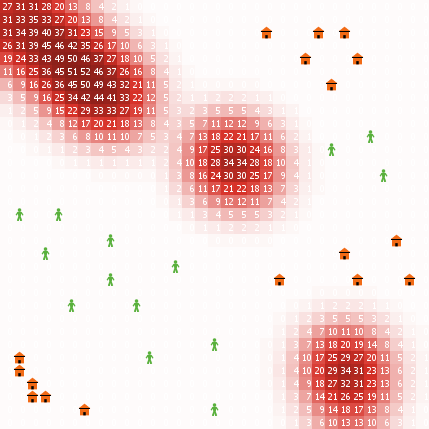
Figure 1 has been created with CoolWorld.nlogo, using NetLogo 4.0.
Figure 2 has been created by clicking on the button  in CoolWorld.nlogo, using NetLogo 4.0.
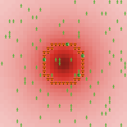
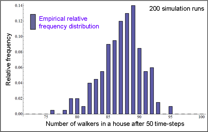
Figure 3 has been created with CoolWorld.nlogo, using NetLogo 4.0. To replicate this experiment, open CoolWorld.nlogo within NetLogo 4.0, go to "Tools" in the menu, then select "BehaviorSpace", and conduct the experiment "figs_3_4_5" twice to obtain two sets of 100 runs.
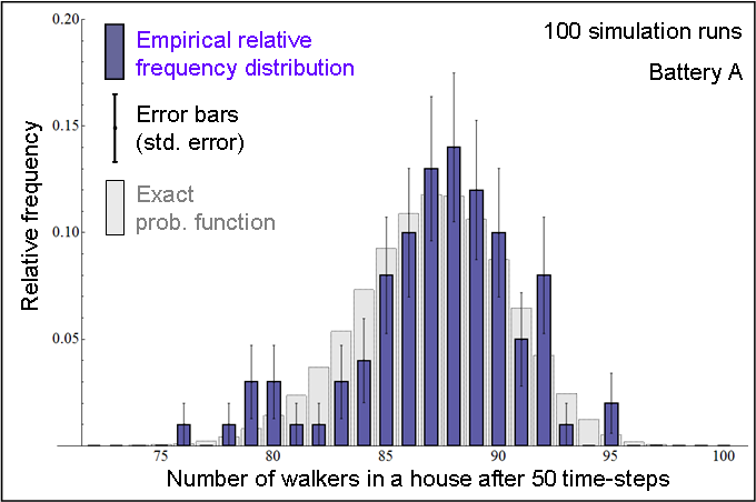
The empirical relative frequency distribution shown in Figure 4 has been created with CoolWorld.nlogo, using NetLogo 4.0. To replicate this experiment, open CoolWorld.nlogo within NetLogo 4.0, go to "Tools" in the menu, then select "BehaviorSpace", and conduct the experiment "figs_3_4_5" to obtain one set of 100 runs.
The exact probability function (in grey) has been computed using this file (CoolWorld-exact-distribution.nb), which has been programmed in Mathematica 6.0.
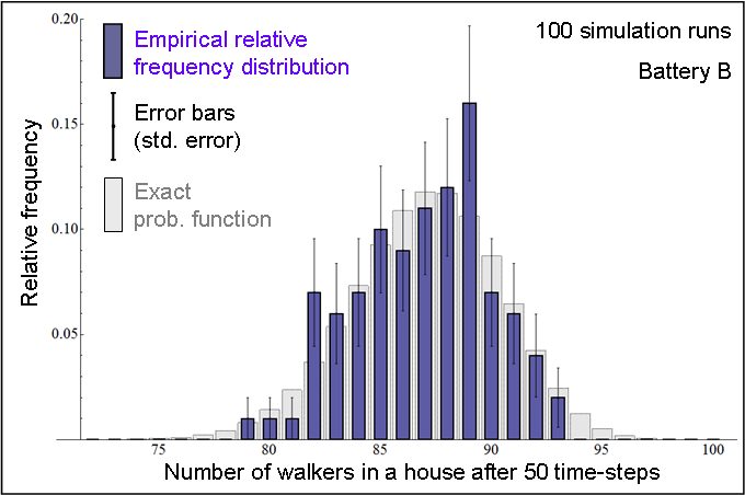
The empirical relative frequency distribution shown in Figure 5 has been created with CoolWorld.nlogo, using NetLogo 4.0. To replicate this experiment, open CoolWorld.nlogo within NetLogo 4.0, go to "Tools" in the menu, then select "BehaviorSpace", and conduct the experiment "figs_3_4_5" to obtain one set of 100 runs.
The exact probability function (in grey) has been computed using this file (CoolWorld-exact-distribution.nb), which has been programmed in Mathematica 6.0.
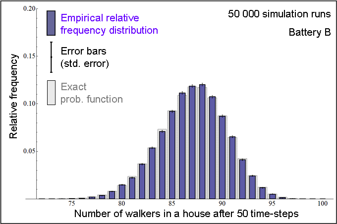
The empirical relative frequency distribution shown in Figure 6 has been created with CoolWorld.nlogo, using NetLogo 4.0. To replicate this experiment, open CoolWorld.nlogo within NetLogo 4.0, go to "Tools" in the menu, then select "BehaviorSpace", and conduct the experiment "figs_6_7" to obtain one set of 50000 runs.
The exact probability function (in grey) has been computed using this file (CoolWorld-exact-distribution.nb), which has been programmed in Mathematica 6.0.

The empirical relative frequency distribution shown in Figure 7 has been created with CoolWorld.nlogo, using NetLogo 4.0. To replicate this experiment, open CoolWorld.nlogo within NetLogo 4.0, go to "Tools" in the menu, then select "BehaviorSpace", and conduct the experiment "figs_6_7" to obtain one set of 50000 runs.
The exact probability function (in grey) has been computed using this file (CoolWorld-exact-distribution.nb), which has been programmed in Mathematica 6.0.
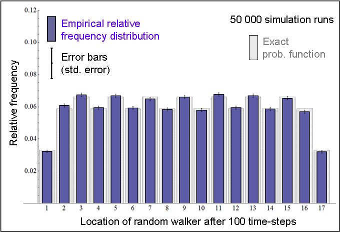
The empirical relative frequency distribution shown in Figure 10 has been created with 1D-Random-Walk.nlogo (applet 1 in the paper), using NetLogo 4.0. To replicate this experiment, open 1D-Random-Walk.nlogo within NetLogo 4.0, go to "Tools" in the menu, then select "BehaviorSpace", and conduct the experiment "fig_10" to obtain one set of 50000 runs.
The exact probability function (in grey) has been computed using this file (1D-RandomWalk-exact-distribution.nb), which has been programmed in Mathematica 6.0.
This (fig11.nb) is the Mathematica 6.0 file we used to produce figure 11. The execution of this program creates a directory named "fig11" where all the figures shown in the animation will be placed. Please make sure you save this file (map.png) in the same directory as fig11.nb before running the program.
Figure 12 has been created with CoolWorld.nlogo, using NetLogo 4.0. To replicate this experiment, open CoolWorld.nlogo within NetLogo 4.0, go to "Tools" in the menu, then select "BehaviorSpace", and conduct the experiment "fig_12". This experiment consists of one single run of 10000 time-steps.
Figure 13 has been created with CoolWorld.nlogo, using NetLogo 4.0. To replicate this experiment, open CoolWorld.nlogo within NetLogo 4.0, go to "Tools" in the menu, then select "BehaviorSpace", and conduct the experiment "fig_13". This experiment consists of 1000 runs of 1000 time-steps each.
This (fig14.nb) is the Mathematica 6.0 file we used to produce figure 14. The execution of this program creates a directory named "fig14" where all the figures shown in the animation will be placed.
This (fig15.nb) is the Mathematica 6.0 file we used to produce figure 15. The execution of this program creates a directory named "fig15" where all the figures shown in the animation will be placed.