©Copyright JASSS

JASSS logo ----

Kerry L. Shaw and Kyle Wagner (2008)

Cricketsim: a Genetic and Evolutionary Computer Simulation

Journal of Artificial Societies and Social Simulation vol. 11, no. 1 3
<https://www.jasss.org/11/1/3.html>

For information about citing this article, click here

Received: 20-Apr-2007    Accepted: 25-Oct-2007    Published: 31-Jan-2008

PDF version


* Abstract

We present cricketsim, an individual-based simulator of species and community dynamics that allows experimenters to manipulate genetic and evolutionary parameters as well as parameters affecting the simulated environment and its inhabitants. The simulator can model genotypic and phenotypic features of species, such as male signals and female preferences, as well as demographic and fitness-related features. The individual-based simulator creates a lattice (cellular) world in which males and females interact by moving, signaling/responding, and mating. One or more species evolves over simulation time as individuals of a species interact with others during its lifetime, possibly creating new offspring through successful mating. The program's design, parameters, execution and data collection are described, an example experiment is presented, and several applications are discussed.

Keywords:
Individual-Based Model, Genetic Algorithms, Communication, Sexual Signaling, Speciation, Evolution, Genetics

* Introduction

1.1
While many lab and field techniques are used to address evolutionary questions, the computer simulation has become a powerful means by which to design and execute experiments and consequently has seen a recent growth in interest and application (Way 2001). Many computational simulations have been used to explore important questions in biology and particularly in evolutionary biology (e.g., Seyfarth 1977; Axelrod 1987; Ikegami & Kaneko 1990; Ventrella 1996; de Bourcier 1996; Gheorghe et al. 2001; Wagner et al. 2001; Wagner & Reggia 2002; Grimm and Railsback 2005; DeAngelis and Wolf 2005).

1.2
In this paper we describe an individual-based evolutionary simulation, called cricketsim, designed to explore the evolution of communication features and the origin and maintenance of species under various external and internal factors. The simulation uses a medium-fidelity representation of genetics; base pairs and codons are not modeled, but individual alleles have a representation along a diploid strand. Some genetic-level processes (recombination and mutation) are represented, while many others (e.g., deletion, transposition) are not. The evolutionary process in the simulation is also medium-fidelity. Mate choice, population dynamics, heredity and diversity are represented. The code is freely available and may be modified by anyone familiar with the java and perl programming languages. Installation instructions, further documentation and the user's manual are available at http://www.bluegradient.org/cricketsim/cricketsim.html. We present a simple pilot experiment to illustrate the program's application.

* Overview

2.1
The cricketsim program is a computer simulation that can be used to explore various evolutionary and genetic questions relating to the evolution of male-female communication and to the origin and persistence of species. Cricketsim offers a graphical user interface (GUI) to the user who sets a large number of parameters and then begins a run of an experiment.[1] It simulates a two-dimensional grid world (a "lattice" world) where each cell in the grid may have a "terrain", or habitat, type and contains one or more individual organisms. Usually the world is filled with two separate, behaviorally distinct, species. One can designate several internal and external mating barriers between the two species, although simulations can be run with no mating barriers whatsoever (in which case we might consider the simulated units to be populations rather than species). Each species is differentiated from others by internal genetic markers as well as genetically-based, measurable traits. Each individual in the world has its own genome, a double-stranded list of values that can be configured to code for several traits, and therefore cricketsim would be best described as a "genetic" model in the terminology of DeAngelis and Wolf (2005).

2.2
Each run of the cricketsim simulation consists of creating a lattice world of a given size and terrain layout, establishing an initial population of organisms of a given species according to the simulator and genotype parameters, and distributing these organisms among the various cells in the world. The simulation proceeds by discrete timesteps wherein each individual performs one or several kinds of actions, having received input determined by its current location and the state of nearby organisms. All outcomes of their actions are computed, after which the next timestep begins. The simulation ends when the maximum number of timesteps has been reached. Offspring do not replace their parents but join the world with parents that have not completed their lifespan. Population size is an outcome of reproduction, longevity, crowding tolerance and size of the world.

* Potential Applications

3.1
Cricketsim was originally designed to simulate the behavior of a real-world system of acoustically diverse crickets that occur in the Hawaiian Islands (Otte 1994; Shaw 2000). Species of crickets in Hawaii are highly diverse, behaviorally distinct, yet, in many cases, very closely related (Mendelson and Shaw 2005). Hawaiian crickets provide systems that naturally lend themselves to studying the consequences of behavioral variation to species interactions and evolutionary diversification.

3.2
There are several major ways in which cricketsim might be employed to test interesting biological questions. Cricketsim was designed to accommodate the study of acoustic communication, but can also facilitate the study of male-female signaling systems in general, a research area of profound importance to understanding the evolution of biodiversity (Mead and Arnold 2004). Because male and female communication traits have separate genetic control, cricketsim qualifies as a "preference" model (Servedio 2000; as opposed to an "assortative mating" model where male and female mating traits are identical). Thus cricketsim allows one to examine the influence of different male and female communication trait values on the future evolution of two or more species participating in a simulation experiment. In addition, cricketsim enables the manipulation of female preference functions for signaling traits in order to examine the effect of preference function shapes (Shaw and Herlihy 2000) on signal evolution and species interactions. Cricketsim also facilitates the direct comparison of pre- and post-zygotic barriers to gene flow in the dynamics of hybrid zones. Moreover, through permutations of the genetic basis of traits underlying each of these systems, cricketsim allows one to explore the effect of the genotype-phenotype relationship on signal evolution and speciation. With cricketsim, one can easily manipulate genetic linkage among these traits as well, thus making it a very exciting and powerful tool for the testing of evolutionary hypotheses at both the phenotypic and genotypic levels. We discuss further advantages of cricketsim in relation to similarly motivated individual-based models in the discussion.

3.3
The following sections describe each aspect of the cricketsim simulator in more detail.

* Cricketsim Methodology

World

4.1
The world that the individuals inhabit is a rectangular grid of cells. Unlike many other artificial life simulations, the cricketsim world is nontoroidal (no wraparounds from one edge to the other) to better simulate realistic geographical constraints. Each cell can contain zero or more individuals. Male individuals send signals continuously that may be heard beyond their current cell (depending on the signal range parameter). Otherwise, individual activity is limited to other individuals within the same cell. Each female compares the signal from each male in her cell to her preference, and she also compares signals from nearby males. If the male whose signal is closest to her preference is in her cell, she remains there and mates with that male; otherwise, she moves to an adjacent cell closer to the male with the best signal. Males use the density of their cell to determine if they will move or stay, and overcrowding in a cell causes the individuals to age more quickly and consequently limits the rate of overall population growth.

4.2
The world's cell-based construction conveniently reduces the complexity of the communication algorithm. If the world were not divided into cells and all individuals were instead located with cartesian coordinates, all male signals would have to be distance-checked with respect to all females, and communication would take O(M*F)[2] operations (M = male population size, F = female population size). When signals are limited only to those females within range, communication takes about O((R×M×F) / (H×W)), where H and W are the height and width of the world, R is the number of cells a male's signal can reach. For populations of about 100 males and 100 females, with R = 9 (signal "radius" of one) and H=W=15. This means that a cartesian-based world would require on the order of 10,000 operations to process male-female communications, whereas the cell-based world only requires on the order of 400 communications.

4.3
Each cell also has a terrain type. Types are simply numbers, but can be thought of as different kinds of ground cover, elevation, temperature ranges, etc. For example, type 1 might be leaf litter in a forest, type 2 might be a grassy plain, and type 3 might be sand dunes. Nevertheless, terrain types differ from each other only in numerical value and have no other distinguishing properties. Individuals attempt to move to terrain types that match their own "ideal" terrain type. So those individuals that prefer grassy plains will move to type 2 cells. If they are already in a type 2 cell, and this is their ideal terrain, then they would normally stay in that cell. An individual in a cell which doesn't match its terrain type will age faster.

4.4
The number of rows (height) and columns (width) of the world can be specified. In addition, the number of terrain types and the distribution of the terrain types across the cells can also be specified. A random layout means that each cell is given a type at random. A "tile size" can be specified so that the random layouts occur in clusters of 2x2, 3x3 or other square cell clusters. A striped layout assigns adjacent columns of cells to the same terrain type. If there were ten columns in the world and five terrain types, a striped layout makes five double-column stripes of cells, each stripe containing cells all of the same terrain type.

Organisms

4.5
Cricketsim is an individual-level simulation; that is, it simulates individuals each with their own independent attributes and examines the emerging and evolving properties of the modeled species (Strand et al. 2002; Sadedin and Littlejohn 2003; Hilscher 2005). Trait values are determined by each individual's genome, the most important property of individuals (detailed below under Genomes). Each individual in Cricketsim is either male or female and inherits its trait values from its parents in a Mendelian fashion. Alleles may differ between parents and offspring through rare mutations (a user-specified probability); recombination among loci may occur (see Genomes section, below). Organisms can vary in fitness through two components: variable longevity and variable mating success.
Longevity

4.6
Individuals are randomly assigned a lifespan at birth, values of which are chosen from a normal distribution (e.g., if mean lifespan were set = 30 with a standard deviation of five, typical longevities would be between 20 and 40). An individual's age is one at birth, and increases one timestep for every timestep the individual is in the simulation. When an individual reaches its lifespan, it dies and is removed from the world. Optimal aging occurs when individuals age one unit per timestep, but external and internal fitness factors can influence longevity.

4.7
Each individual has an internal lifespan penalty determined by its genome. This value, along with a weighting parameter provided to the simulator, determines how much the individual ages during each timestep beyond the normal rate of aging. For example, if an individual's internal lifespan penalty is zero, it will age optimally at one timestep per timestep spent in the world. If its internal lifespan penalty is four, on the other hand, the individual will age 1+4=5 timesteps per timestep spent in the world. A user-provided constant can be set to any value to magnify or minimize this effect. If that constant is set to zero, crickets will suffer no aging penalty from their internal lifespan values.

4.8
In addition to internal lifespan penalties, each individual has an external lifespan penalty determined by its genome, stemming from its ideal terrain type. For simple worlds with 2 terrain types (TT=1 and TT=2), all individuals will have an ideal terrain type that is within this range. An individual's ideal terrain type (cTT) is actually a real value, in this case 1 ≤ cTT ≤ 2. For example, pure species individuals could have cTT=1 or cTT=2, while hybrids between them might have some value in between (a hybrid of these two species would have a cTT=1.5). This terrain factor can affect an individual's rate of aging. If the individual is in a cell such that TT=cTT, then it has no extra lifespan penalty. However, an individual in a cell with non-ideal terrain would age more than the normal one unit per timestep spent in the simulation. The external lifespan penalty is K × |cTT-TT|, where K is a constant provided by the user. If K=0, the external lifespan penalty would never be a factor in that particular run. Terrain type partially determines organism movement: if an individual's ideal terrain type doesn't match its current terrain type, and it can find a better terrain type in an adjacent cell, it will move to that type. Otherwise, it will stay and suffer a lifespan penalty.

4.9
A lifespan penalty can also occur for males under conditions of overcrowding. Each timestep, males will move or stay partially depending on the density of males in their current cell. A user-defined value specifies the ideal density, and a male in a cell with fewer or more males will move from that cell to an adjacent cell with a more ideal density. Overcrowding in a cell causes the individuals to age more quickly, at a rate specified by the user. The user can also specify whether terrain or density-based movement is prioritized.

4.10
Finally, females move based on terrain types as above, and on which male signal they prefer (see below). The user can likewise specify whether terrain or signal-based movement is prioritized.
Mating success

4.11
Male and female fitness can also vary according to how many matings they achieve, which will depend in part on user-determined preference functions. Females hear all males who signal near them based on male signal range, which is user-defined. Each female chooses to whom she responds on the basis of her preference function and the degree to which her preference value matches the male signal. The female preference function is a user-defined parameter, allowing one to test evolutionary outcomes as a function of how females make mating decisions. The function is computed by calculating a lower and upper range for the acceptable signal value (SV) of the male given the female's preference value (PV). If the male's SV falls within the allowed range, the female will consider the male. The female will choose the male whose SV is closest to her actual PV (with the exception of open-ended functions, see below). There is a user-supplied constant, C, the tolerance, which affects some of the functions. Available female preference functions include 1) best-proportional, where the female responds to the male whose signal is closest to her preference, with higher preference values accompanied by larger ranges of tolerance (PV-(PV/C) ≤ SV ≤ PV+(PV/C)); 2) best-inverse-proportional which is similar to best-proportional, but tolerance for signal deviations decrease as preference values increase (PV-(C/PV) ≤ SV ≤ PV+(C/PV)); 3) best-fixed where female tolerance for signal deviations does not vary with preference values (PV-C ≤ SV ≤ PV+C); 4) open-ended increasing, where the female responds to the male with the highest signal(SV ≥ PV); and 5) open-ended decreasing, where the female responds to the male with lowest signal (SV ≤ PV). A difference between the male's signal and the female's preference is computed, and if the difference is too great (based on her preference function), she will reject the male entirely, even if he has the best signal nearby. Otherwise, the preference function gives a "score" to each male's signal, and the female moves toward /mates with the male with the best score according to her preference function.

4.12
For example, in an acoustic system such as crickets display, if female 1 has a PV of 1.0, female 2 has a PV of 3.0, and a male sings at a SV of 2.0, the difference between the PV and the SV are computed; both differences are 1.0. For a best-fixed preference function, both females would have the same response to the male (either both would reject him or both would accept him, depending on the user-defined "preference function tolerance"). For best-proportional, female 1 would be less likely to accept the male than female 2 since her tolerance range is smaller - her PV is less than female 2's. For best-inverse-proportional, the opposite is true. The actual result (accept/ignore) would depend on the "preference function tolerance" parameter. For open-ended-increasing, female 1 would accept the male while female 2 would reject him (his SV is below her PV). The opposite result would be the case for open-ended-decreasing.

4.13
Individuals can reproduce immediately upon entering the world. When a female has decided to mate with a male (they must both be in the same cell for this to happen), they produce a random number of offspring, chosen from a normal distribution whose parameters are user-defined. Each offspring is produced by combining a randomly drawn, recombinant, chromosome from each parental individual, creating a new, diploid offspring. These new individuals are placed randomly in the world, within a user-determined radius of their parents, dictated by several user-defined parameters. Offspring join the world with parents that have not completed their lifespan. After mating, females can not mate until the refractory period (e.g., ten timesteps) has elapsed for them — another user-defined value.

Genomes

4.14
Each individual has a genome, which codes for its traits: sex, signal value, preference value, internal lifespan, and ideal terrain type. The values for each individual's genome come from its parents through recombination and through occasional mutations. The initial population's genomes (i.e., the alleles) are randomly generated, but they are constrained by distributions and min/max values.

4.15
Each individual's genome is diploid, with a total haploid length of 100.0 units. The number of loci and locus distributions in a genome are determined by user-defined parameters before the run begins (see below). The genomes of all individuals will have the same distribution of loci, even though the alleles at these loci may vary. To reproduce, each parent contributes one recombinant chromosome to its offspring. Recombination coincides with each reproductive event via a 1-point crossover. To achieve recombination, a random point is chosen on the chromosomes within each parent, the chromosomes are cut and alleles at each locus along the chromosome string to one side of the cut site are swapped between the chromosomes. One recombinant chromosome is chosen at random from each parent to make up the individual offspring.

4.16
Each gene is associated with a locus, the sole purpose of which is to make recombination among loci more spatially realistic. The alleles are stored in a list, but each allele is associated with a locus so that even if it is adjacent to another allele in the list, its "virtual" genomic location may be far away (discussed in more detail below). This would imply, in such a case, that a crossover might occur between two distantly located alleles, even if they are adjacent in the list of alleles coding for this individual. The justification for using virtual loci is to enable user defined distributions of loci across the genome. The location of loci underlying a trait will affect the degree to which recombination between them can occur, and thus the degree to which they evolve independently or as a unit. While a real organism's genome would contain many more genes than the individuals in our simulation, they do not play a functional role in this simulation. Nonetheless, we have facilitated the placement of the genes that do play a functional role (e.g. signal, preference, endogenous/exogenous fitness) at various virtual locations across the genome simulating the effect of a genome interspersed with other genes.

4.17
An example, shown in Figure 1, of a short, simple genome will help to illustrate possible genome content.


Chromosomal
location
0.557.265.974.187.087.287.499.0
allele10.30.10.40.21.01.02.0“X”
marker1AAAAAABA
allele20.20.20.280.191.02.01.0“O”
marker2AAABABAA

Figure 1. A short example genome from a male hybrid organism. Chromosomal location refers to the location on the chromosome of 100.0 units. The sex locus is positioned at 99.0 units. The signal loci are positioned at 0.5 and 57.2 units. The preference loci are positioned at 65.9 and 74.1 units. The fitness loci (for internal and external lifespan penalties) share the remaining loci at 87.0, 87.2, and 87.4 units.

4.18
In Figure 1, the individual has eight loci and two alleles per locus in its genome. The first locus contains 0.3 and 0.2 as values. The next locus is adjacent to the first, but is located almost half the total virtual length of the genome away from that first locus. Thus, recombination is more likely to happen between these two loci than between any other loci in this genome. These loci are specified by the user; each location is a real-valued number between 0.0 and 100.0, and each gene must have a unique locus to be placed along the genome.

4.19
Each allele also comes with a marker. In a single species simulation, this has no utility, but is very useful in a two-species simulation where hybrids may arise. Markers allow the user to track the species' origin of various alleles that make up the hybrid individual's genotype. For example, suppose alleles from the first and second species are marked with "A" and "B", respectively. With the "birth" of each individual, its overall "hybridity" can be determined by calculating how many loci have both "A" and "B" alleles, and then determining whether "A" or "B" is in the majority. In the example above (Figure 1), the genome mostly orginates from species "A", but there is hybridity at three loci. So the genome of this individual can be considered 81.25% (13/16) "A".

Encoding of traits

4.20
When setting up a simulation, the user can specify some architectural aspects of the genome. However, all individuals in a run, regardless of species, have the same genetic structure. This enables any individual from any species to breed with another during the simulation run, even if their offspring have poor fit to their environment. Each genome has one sex locus at a user-specified location. The value for an allele at the sex locus is either "X" or "O" (absence of the "X" allele). Females are "XX", while males are "XO" or "OX". "OO" is prevented by the simulator.

4.21
Both the number and virtual locations of male signal and female preference loci are user-specified. Initial values for alleles at these loci (for the initial population of individuals added to the world) are randomly generated from normal distributions whose means and standard deviations are also user-specified. The value of an allele at these loci can change between parent and offspring through the user-specified mutation rate, or the probability, per allele, that an allele's value will change when being passed on to an offspring. Individuals have NSV loci that encode for signal value (SV). The SV trait for an individual is calculated simply by adding up all of its SV alleles. The same is true for signal preference.

4.22
The number and virtual locations of lifespan penalty (internal fitness) and terrain type (external fitness) loci are also user-specified. Initial values for alleles at these loci are user-specified and constant for a given species. In addition, they remain unchanged throughout the simulation, and are not subject to mutation. An individual's internal lifespan penalty is calculated by sampling a user specified number of pairs of fitness loci. If there were five fitness loci, two loci would be chosen at random (with replacement) from this set and assessed for mismatches both within loci (i.e., are the alleles the same or different?) and between loci within each chromosome (i.e., are the alleles the same or different?), yielding four possible mismatches. Then another two loci would be chosen and assessed for mismatches. The parameter "#pairs of age loci to sample for heterozygosity" specifies how many pairs will be chosen in this manner. The total number of mismatches is the individual's "fitness mismatch score", or Sf. This value is multiplied by the "genetic age factor" parameter to determine how many extra timesteps the individual will age for every timestep spent in the world. Because the values for alleles at these loci are constant within a species, pure species individuals will never experience an internal lifespan penalty. However, this system provides a mechanism to lower the fitness of hybrid offspring, consistent with current speciation genetics theory and evidence (Brideau et al. 2006). It can also be set to zero if no internal fitness penalty is desired.

4.23
An individual's ideal terrain type (which might serve as an environmentally-based fitness penalty or mating barrier between species) is determined using the same "fitness loci" as for the internal fitness penalty. This trait's value is simply the average of all of the alleles found at these loci.

4.24
An example genome will show how cricketsim computes traits from the genome. Figure 1 shows a male hybrid genome with several alleles coding for each trait of an organism. Cricketsim must build a phenotype from the genome, extracting sex (locus 99.0), signal (loci 0.5 and 57.2) or preference (loci 65.9 and 74.1), internal fitness penalty and ideal terrain type traits (sharing the same loci at 87.0, 87.2 and 87.4). Because the individual is male, it will express the signal trait. Adding up all alleles (at positions 0.5 and 57.2 units) results in a signal value of 0.3+0.2+0.1+0.2 = 0.8. The individual's signal preference would be 0.4+0.28+0.2+0.19 = 1.17, but since the individual is male, it will not express preference. However, it will still pass these genes on to its offspring.

4.25
The individual's internal lifespan penalty is calculated by selecting several pairs of loci and comparing them for mismatches. Among loci 87.0, 87.2 and 87.4, suppose that two pairs are to be chosen ("#pairs of age loci to sample for heterozygosity" = 2). Let the first pair be <87.0,87.4>; the first locus has no internal mismatch ("Allele1" vs "Allele2"), the second does (1.0 is not the same as 2.0), and there is a mismatch in "Allele 1" across loci 87.0 and 87.4, but no mismatch between Allele 2 at loci 87.0 and 87.4. So there are two mismatches in total from this pair. A second pair of loci might be 87.2 and 87.4. There are mismatches within each locus, and mismatches across each locus, making four mismatches. The total is six mismatches, and with the parameter "Genetic age factor" set to 0.3, the organism ages one extra timestep (6×0.3=1.8, rounded down to 1) per timestep it is in the world.

4.26
The organism's ideal terrain type is computed by adding up all alleles at the same loci as those underlying the internal fitness penalty. This organism's ideal terrain type is (1.0+1.0+1.0+2.0+2.0+1.0)/6=(8.0/6)=1.25. Thus, the individual is more at home in TT=1 than TT=2, but it might still incur a small age penalty even in TT=1 (depending on the size of the "Terrain sensitivity" parameter).

Primary Parameters for Experimentation

4.27
Cricketsim is highly configurable. There are many parameters that affect the world or the simulator itself. The user can determine the dimensions of the world, terrain types and layout. In addition, the various internal and external aging penalty factors, male and female behavioral parameters (e.g., signal range, female preference algorithm, male and female movement priorities, male density parameters and female mating latency), and general demographic parameters (e.g., number of offspring per mating, offspring dispersal and optimal longevity) are flexible. The genetic basis of signaling and preference traits, and of fitness traits can be varied as well. In contrast to world and simulator parameters, some parameters affect all individuals across all populations in a simulation run, such as the genetic features of mutation and recombination and the genetic architecture of traits (i.e. the location and number of loci underlying specific traits).[3] Genetic architecture parameters must apply to all individuals so that individuals from different species will have compatible genomic structures to facilitate interbreeding.

4.28
Finally, each genotype and species must be specified. Each species can be associated with a different genotype, although two species can use the same genotype if so desired. Genotype parameters specify, for each genotype desired, what marker (e.g. A or B) will be associated with the genes of the individuals in the initial population associated with the genotype (these markers are used for data analysis to calculate hybridity). These parameters also specify the initial normal distributions from which the signal and signal preference genes' alleles will be sampled. Similarly, species parameters specify which genotype will be associated with initial members of the simulation run. Species parameters indicate how and where the initial individuals will be placed (clustered tightly in one spot or spread loosely around the world). Any hybrid offspring from two different species will not possess the original genotypes, but instead will possess some mixture of the two.

4.29
Cricketsim also has program-specific parameters (locations of datafiles, etc.) and display parameters: cricketsim can display real-time graphs and world views if desired, though at an appreciable slowdown in computation.

Data Collected

4.30
Data are collected at every timestep of the simulation. These data are comprised of tallies, averages, computations and snapshots of various states of the individuals, subpopulations, the whole population and the world.

4.31
The primary forms of data collected are data per individual, data for each species (based on genetic categorizations), data for males, data for females, and data on the spatial layout of the individuals. Individual-based data consist of averages of how many offspring were produced by each individual in its lifetime, and the signal and preference values of the individuals. Population-based data include classifying each individual (over time) into a histogram bin based on its "relative hybridity" (how "pure" of an "A" or "B" genome it has), and then computing mating success or number of individuals for each bin.

4.32
Spatial data attempt to show the spatial distribution of individuals based on their predominant genotype ("A" or "B"). Since most individuals will be at least partially hybrid after the simulation has run for a while, these classifications are only approximate.

4.33
Cricketsim outputs data to files, and it can graph most of these data real-time. Although this slows down the simulation, it can be very instructive to watch the population dynamics play out over the world or through changing hybridity graphs (see Figures 2 through 4).

Figure
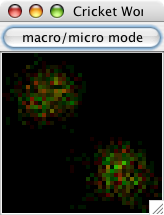
Figure 2. Screenshot of a 40×40 world after 25 timesteps, showing male and female densities in each cell (males are red, females are green, cells with a mixture have an interpolated color value between red and green). Black areas indicate that no crickets are in that cell. This is the "micro" mode display, showing information only about male/female densities. Each population began in a tightly-clustered area and has started to grow outwards.

Figure
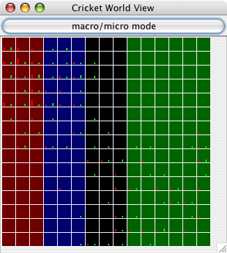
Figure 3. Screenshot of a 15×15 world after a few timesteps have elapsed. This is the "macro" mode display, which shows more information about each cell. Each cell displays its terrain type as a color (there are four terrain types in this particular run). Also, each cell has a bar whose height corresponds to the number of males (red) and females (green) in that cell. Notice that the fringes of each population cluster tend to be male-only or female-only and sparsely populated, while the center of each population (upper left and lower right) contains many males and females.

Figure
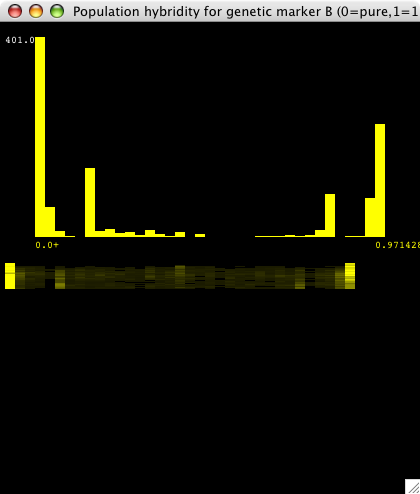
Figure 4. This is a real-time histogram of hybridity with respect to the "B" genetic marker (the marker for population 2). The tall bars at either end indicate that most individuals are either pure B (at 0.0) or pure A (at 0.97, which is a histogram bin containing 0.97 to 1.0 hybridity individuals). There are some significant hybrid populations as well. The "smear graph" below shows slices of the above histogram over time, with t=0 at the top. At t=0, and for a while, there are no yellow bars in between 0.0 and 1.0 except at the ends, so both populations are pure. As time goes on, some hybrid matings occur, which is reflected by the dim yellow bars that appear. The intensity of the bars corresponds to the height of the histogram at that point. This smear graph shows how the hybridity histogram changes over time.

* Pilot Experiment

5.1
To illustrate the use of cricketsim in an experimental setting, consider the question: if two species of cricket were placed in a world with two very different terrain types (say grassy versus a forest habitat), and each species was better adapted to one type, but both species used the same signal and preference values, would their signal and preference values change over time? In other words, would fitness associated with terrain type indirectly cause selection for signal and preference divergence? Cricketsim was run ten times under these conditions. Each population was given identical parameters except for their ideal terrain type (species "A" lived best in terrain type one, while species "B" lived best in terrain type two). The initial individuals from each species were given signal/preference alleles from the same normal distribution. Thus, there was initial variation (for example in signal pulse rate and pulse rate preference) in each population, but that variation was similarly distributed within each species. A control was run with the same parameters except that there was no penalty for terrain type differences (i.e., no external fitness penalty).

5.2
Following are the specific parameters used in this pilot experiment. The world was 15×15 cells, with the left half of the world being terrain type one and the right half being terrain type two. Each simulation ran for 5000 timesteps. Terrain sensitivity was 1.0 (this constant is multiplied by the external lifespan penalty — due to the discrepancy between ideal terrain type and actual terrain type experienced in a given timestep), internal lifespan penalty was 2.0 (moderately selecting against hybrid offspring) and females were expressing the best-proportional preference function (tolerance=2.0). Mean lifespan was 32 time steps, with a ten timestep mating latency for females. Each mating produced ten offspring, dispersed within a three cell radius of their parents. Each cricket's genome devoted eight loci to pulse rate (tightly grouped in locations 5.1 through 5.8), eight to pulse rate preference (tightly grouped in locations 35.1 through 35.8), and ten randomly located loci for internal and external fitness calculations. The sex allele was at location 95.0.

5.3
Two separate genotypes were used - one per species. They differed only by their terrain-type allele (1 or 2, to correspond to terrain types 1 and 2). The alleles for pulse rate and pulse rate preference for the initial species were chosen from a normal distribution with a mean of 0.15 and a standard deviation of 0.05; thus, both species had initial pulse rates and preference means of 0.15×8×2 (8 loci per trait, diploid), or 2.4 pulses per second. Fifty males and 50 females of each species were created in a tight cluster, but the two species clusters were far apart, one on each terrain type (the type that fit the initial population).

Results

Figure
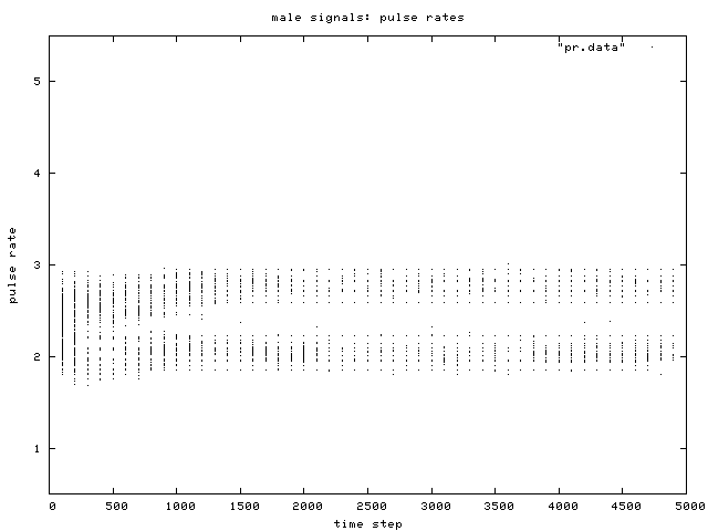
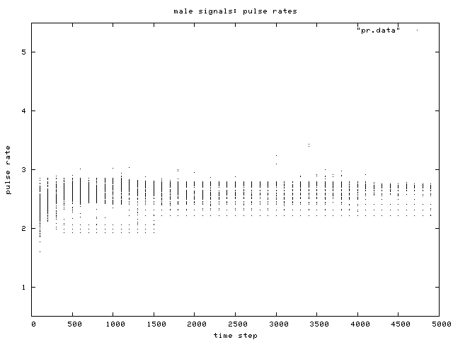
Figure 5. Scatterplot of individual male signal pulse rate values over time, for one simulation run. Two phenotypic groups are clear after about generation 500.

Figure
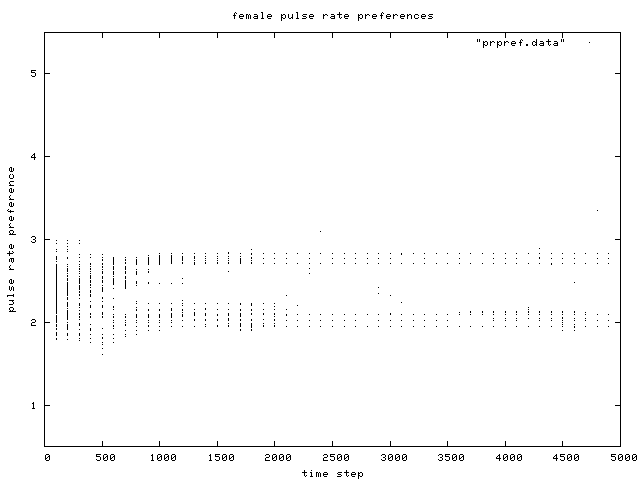
Figure 6. Scatterplot of individual female pulse rate (signal) preferences over time, for the same simulation run as in Figure 1. Like male pulse rate, two preference groups are clear after about generation 500.

Figure
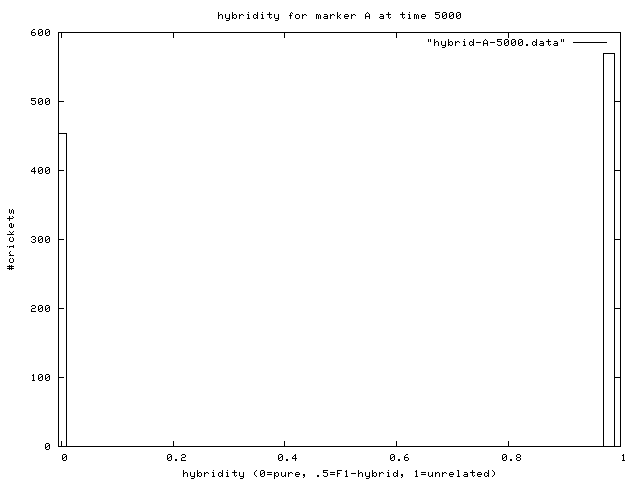
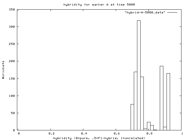
Figure 7. Hybridity of one experimental population at end of simulation. Pure A (right stack) and B (left stack) individuals are evident.

5.4
The purpose of the pilot experiment was to show how to use cricketsim. These results will show some of the data and measurements that cricketsim can produce, although a statistical analysis and full discussion of the results are beyond the scope of this paper. All data shown in Figures 5-8 are from a single simulation run. Ten runs of the simulation were made. In eight of ten runs, the two populations showed a clear divergence in male pulse rates (see Figure 5) as well as in female pulse rate preferences (see Figure 6); the other two runs show variation in signaling, but a more complex statistical analysis would be needed to demonstrate actual divergence between the two species. Importantly, the female preference values matched those of the male signal value within each species. Therefore, the species have diverged from each other in both pulse rate and preference, but both male and female traits remain matched within their respective species. The hybridity graph in Figure 7 shows that the "A"s are genetically distinct from the "B"s. In these simple experiments, the As are all expressing a very similar pulse rate/preference, and this is quite distinct from the pulse rate/preference of the Bs. From these results, the spatial distribution of the different population types at the start and end of the simulation (see Figure 8) and from other cricketsim data (not shown here for brevity), it is clear that the two species, initially only separated by location and genetics, are still separated by these factors, but are now also separated by their pulse rate/preference traits. A single control is shown here (see Figures 9, 10 and 11), suggesting that, in the absence of a penalty for terrain types, the two initial species will generally merge and become a hybrid swarm.


- A A A A - - - - - - - - - -
A A A A A A - - - - - - - - -
A A A A A A A - - - - - - - -
A - - A A - - - - - - - - - -
A - - - - - A - - - - - - - -
- - - - - - - - - - - B - - -
- - - - - - - - - - B - B - B
- - - - - - - - - B B B - B -
- - - - - - - - - - B B B B -
- - - - - - - - - B B B B B B
- - - - - - - - B B B B B B B
- - - - - - - - - B B B B B B
- - - - - - - - - - B B B B B
A A A A A A A A A - A A A A A
A A A A A A A - A A A A A A A
A A A A A A A A A A A A A A A
A A A A A A A A A A A A - A A
A A A A A A A A A A A A A A A
B B B A A B B B B A B B B B -
B B B B B B B B B B B B A B A
B B B B B A B B B B B B B - A
B B B B B B B B B B B B A B B
B B B B B B B B B B B B B B B
B B - B B B B B B B B B B B B

Figure 8. Initial and final spatial distribution of population types (A=more than 50% genes from A population, B=more than 50% genes from B population).

Figure
Figure 9. Scatterplot of individual male signal pulse rates over time, for one simulation run, control condition.

Figure
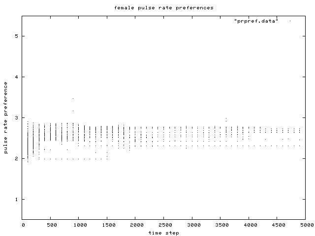
Figure 10. Scatterplot of individual female pulse rate (signal) preferences over time, for the same control condition simulation run as in Figure 6.

Figure
Figure 11. Hybridity of one control population at end of simulation. The hybridity of individuals is distinctly bimodal, although no splitting was evident in the signal and preference phenotypes.

* Discussion

6.1
The inspiration for cricketsim's world and inhabitants came from the extensive species diversity of crickets that are endemic to the Hawaiian islands (Otte 1994; Shaw 2000). The simulation was designed to explore genetic and evolutionary outcomes for small populations faced with the problem of finding genetically compatible mates in heterogeneous environments. On the one hand, cricketsim could simulate the dynamics of a great many species in a variety of situations. On the other hand, its results apply best to species that attract mates using a unique signal, have large family sizes with no parental care, and whose longevity depends primarily on some internal compatibilities or an environmentally-based fitness trait. This makes cricketsim applicable to some arthropods, fish, amphibians and reptiles, i.e., any system wherein the primary survival challenges can be modeled by a single spatial variable and/or some genetic incompatibilities between species.

6.2
Cricketsim allows an investigator to manipulate environmental, genetic and demographic variables in order to test evolutionary hypotheses, with an emphasis on speciation - its origin, maintenance, and evolution. Unlike population-level simulations and models (such as Lotka-Volterra's differential equations for population modeling, Lotka 1925,Volterra 1926), cricketsim is an individual-based model. Individual-based models can mimic the genomic basis of traits underlying individual behavior and have been considered more flexible than population-level models (DeAngelis and Wolf 2005). While both kinds of models have their uses (Grimm and Railsback 2005), individual-based models facilitate analysis of individual behaviors and properties, and the granularity needed to support population-level hypotheses using individual-level manipulations (see Henson et al. 2001 for other issues affecting population-level models).

6.3
The strength of the individual-based model, where questions about phenomena at a higher level are affected by the manipulation of variables at a lower level, are illustrated by our pilot experiment. Two populations evolved different pulse rates and preferences due to strong selection on different terrain types. The resulting pulse rates of these populations were an outcome of the simulation rather than an input variable. The selection pressures that caused evolution to occur came from a combination of an individual's lifespan penalty for being in the "wrong terrain" and the individuals' mate choice and resulting reproductive success. Experiments such as these must be compared to controls to show that the results are not inevitable. In this case, we saw different outcomes showing that certain results are not inevitable. Controlled experiments are crucial using the computer simulation methodology, just as they are in lab and field experiments. And, as with any good experiment, results are always stronger when supported by divergent approaches (e.g.,Schmitz 2000). Ideally, a computer simulation approach would be performed alongside lab and field experiments, possibly followed by a mathematical model to succinctly describe the phenomenon. A computer simulation may be performed before lab/field work to inspire empirical hypothesis testing, as a cost-saving or risk-mitigating measure, or it may be performed simultaneously or afterwards to provide support for a hypothesis.

Cricketsim Advantages

6.4
Cricketsim shows some advantageous differences to previously published individual-based models, particularly with respect to the flexibility of the genotype-phenotype relationship of traits. Some of these advantages are outlined below. For example, cricketsim enables the separate genetic coding of male and female traits (i.e., a "preference" model in the terminology of Servedio (2000), as opposed to an "assortative mating" model, e.g. Doebili and Deickmann (2000)). In addition, cricketsim allows for a variable number of loci valued between zero to effectively infinity by allowing alleles to take on non-integer values. In their simulation of sexual communication, Sadedin and Littlejohn (2003), model a specified ten loci, each containing alleles valued at zero or one, limiting integer trait values to between zero and 20. Furthermore, in cricketsim the chromosomal locations of loci (and thus their linkage relationships) are highly flexible, unlike Sadedin and Littlejohn's model which is limited to an absence of chromosomal linkages. Similar genetic constraints are found in the model of Hilscher (2005). While the above mentioned models were designed for specific applications, cricketsim has considerable flexibility to examine how the future evolution of two or more species might be affected by different male and female communication trait values, different levels of quantitative genetic control, and different degrees of linkage both within and between the male and female traits. Thus, one of the most exciting and powerful advantages of cricketsim is that it can explore the effect of varying genetic structures underlying the genotype-phenotype relationships on evolutionary outcomes.

6.5
Cricketsim is also distinctive in offering both internal (i.e., environment-independent) and external (i.e., environment-dependent) sources of variable individual fitness, each of which can be in effect alone, or with the other. Fitness variation can also be eliminated altogether. While Hilscher's (2005) model simulates an external fitness function, Sadedin and Littlejohn's (2003) simulates an internal fitness function, and neither model enables both sources of variable fitness. In addition, the variable fitness effects are realized in cricketsim with the possibility of overlapping generations, unlike the above-mentioned models.

6.6
Cricketsim possesses some algorithms and data structures that may be of additional interest. First, cricketsim uses a cell-based limit "radius" to contain events (e.g. signals). Thus, a male may send a signal, but it doesn't have to be processed by every female in the world (which would take time proportional to the square of the population size). Instead, a male's signal is localized to nearby females (with the radius parameter). Second, the program is implemented independently of the graphical interface, using a Model-View-Controller (MVC) Pattern. Because the simulation "engine" is separate from the parameter input windows, the buttons and the real-time output graphs, cricketsim can be modified for uses beyond its original purpose and new simulations can be built from the cricketsim code. Finally, the code underlying the genome/chromosome is flexible, allowing for any kind of structure to be built. While the current version of cricketsim simulates one diploid chromosome, the code provides for any number of chromosomes of virtually any ploidy level. The main cricketsim engine could be modified to accommodate, e.g., 23 diploid chromosomes of varying lengths and structures, such as are found in humans.

6.7
In summary, cricketsim simulates a diversity of interactions common to many species: movement, mate choice and the use of a signaling trait to attract and select a mate. It can be used to investigate hypotheses for evolution, population dynamics, genetics, and especially speciation. Cricketsim provides real-time graphical analysis and plots of population measures, geographical distributions, genetic and phenotypic diversity and hybridity. The simulation is open-ended in that it simulates actions of individuals in the world, the effect of genetic variation in the world and interactions among individuals. Cricketsim also can measure the change in individual traits and thereby monitor the effect of many variables on evolutionary outcomes.

* Acknowledgements

We thank three anonymous reviewers for comments that helped improve the manuscript. Kyle Wagner would like to thank Bill Timberlake, Mike Gasser and Jim Reggia for many helpful discussions of the proper application of simulation results to real scientific questions. Kerry Shaw would like to thank members of her lab for many stimulating discussions on the topic of speciation.


* Notes

1 Cricketsim can also be run in batch (i.e., non-interactive) mode, meaning that it can be run from a command-line script; batch mode allows an experiment to be repeated many times with a single command. This capability is documented in the code, which can be found at the program's website.

2 Big-O notation expresses the order of magnitude of work that an algorithm must perform. O(N) would mean that an algorithm operating on N items would require cN steps, where c is a numerical constant. Given small enough values of c (quite typically the case), an O(N) algorithm is much better than an O(N^2) algorithm.

3 Please refer to http://www.bluegradient.org/cricketsim/cricketsim.htmlfor a full description of these parameters as well as the many other parameters which can be set in the program.


* References

AXELROD, R (1987). "The evolution of strategies in the iterated prisoner's dilemma". In Davis L (Ed.) Genetic Algorithms and Simulated Annealing, Los Altos, CA: Morgan Kaufmann.

BRIDEAU, N J, Flores, H A, Wang, J, Maheshwari, S, Wang, X, Barbash, D A (2006). 'Two Dobzhansky-Muller genes interact to cause hybrid lethality in Drosophila'. Nature 314: 1292-1295.

DEANGELIS, D L, Mooij, W M (2005). 'Individual-based modeling of ecological and evolutionary processes'. Annual Reviews of Ecology and Systematics 36: 147-168.

DE BOURCIER, P (1996) 'Using a-life to study bee life: the economics of central place foraging'. In Maes, P et al. From Animals to Animats 4 ed. Bradford/MIT, MA.

DOEBILI, M, Deickmann, U (2000). 'Evolutionary branching and sympatric speciation caused by different types of ecological interactions'. American Naturalist 156: S77-S101.

GHEORGHE, M, Holcombe, M, Kefalas, P (2001). 'Computational models of collective foraging'. BioSystems 61: 133-141.

GRIMM, V, Railsback, S F (2005) Individual based modeling and ecology. Princeton, NJ: Princeton University Press.

HENSON, S M, Costantino, R F, Cushing, J M, Desharnais, R A, Dennis, B, King, A A (2001). 'Lattice effects observed in chaotic dynamics of experimental populations'. Science 294: 602-605.

HILSCHER, R (2005). 'Agent-based models of competitive speciation I: effects of mate search tactics and ecological conditions'. Evolutionary Ecology Research 7: 943-971.

IKEGAMI, T, Kaneko, K (1990). 'Computer symbiosis: emergence of symbiotic behavior through evolution'. Physica D 42: 235-243.

LOTKA, A J (1925) Elements of physical biology. Baltimore, MD: Williams & Wilkins Publishing.

MEAD, L S, Arnold, S J (2004). 'Quantitative genetic models of sexual selection'. Trends in Ecology and Evolution 19: 264-271.

MENDELSON, T C, Shaw, K L (2005). 'Rapid speciation in an arthropod'. Nature 433: 375-376.

OTTE, D (1994) The Crickets of Hawaii: Origin, Systematics, and Evolution. Orthoptera Society/Academy of Natural Sciences of Philadelphia.

SCHMITZ, O J (2000). 'Combining field experiments and individual-based modeling to identify the dynamically relevant organizational scale in a field system'. Oikos 89: 471-484.

SADEDIN, S, Littlejohn, M J (2003). 'A spatially explicit individual-based model of reinforcement in hybrid zones'. Evolution 57: 962-970.

SERVEDIO, M R (2000). 'Reinforcement and the genetics of nonrandom mating'. Evolution 54: 21-29.

SEYFARTH, R M (1977). 'A model of social grooming among adult female monkeys'. Journal of Theoretical Biology 65: 671-698.

SHAW, K L (2000). 'Further acoustic diversity in Hawaiian forests: Two new species of Hawaiian cricket (Orthoptera: Gryllidae: Laupala)'. Zool. J. Linn. Soc. 129: 73-91.

SHAW, K L, Herlihy, D P (2000). 'Acoustic preference functions and song variability in the Hawaiian cricket Laupala cerasina'. Proceedings of the Royal Society of London B 267: 577-584.

STRAND, E, Huse, G, Giske, J (2002). 'Artificial evolution of life history and behavior'. American Naturalist 159: 624-644.

VENTRELLA, J (1996) "Sexual swimmers: emergent morphology and locomotion without a fitness function". In Maes, P, Mataric M J, Meyer J-A, Pollack J, Wilson, S W (Eds.) From Animals to Animats 4, Bradford/MIT, MA. Pp 484-496.

VOLTERRA, V (1926). 'Variazioni e fluttuazioni del numero d'individui in specie animali conviventi'. Mem. R. Accad. Naz. dei Lincei. Ser. VI(2).

WAGNER, K, Reggia, J (2002). 'Evolving consensus among a population of communicators'. Complexity International, 9, http://www.complexity.org.au/ci/vol09/wagner01/wagner01.html.

WAGNER, K, Reggia, J, Wilkinson, G, Uriagereka, J (2001). 'Conditions enabling the emergence of inter-agent signaling in an artificial world'. Artificial Life 7: 3-32.

WAY, E (2001). 'The role of computation in modeling evolution'. BioSystems 60: 85-94.

----

ButtonReturn to Contents of this issue

© Copyright Journal of Artificial Societies and Social Simulation, [2008]