Umberto Gostoli (2008)

A Cognitively Founded Model of the Social Emergence of Lexicon

Journal of Artificial Societies and Social Simulation vol. 11, no. 1 2
<https://www.jasss.org/11/1/2.html>

For information about citing this article, click here

Received: 31-May-2006    Accepted: 28-Sep-2007    Published: 31-Jan-2008

Abstract

This paper suggests a model of the process through which a set of symbols, initially without any intrinsic meaning, acquires endogenously a conventional and socially shared meaning. This model has two related aspects. The first is the cognitive aspect, represented by the process through which each agent processes the information gathered during the interactions with other agents. In this paper, the agents are endowed with the cognitive skills necessary to categorize the input in a lexicographic way, a categorization process that is implemented by the means of data mining techniques. The second aspect is the social one, represented by the process of reiterate interactions among the agents who compose a population. The framework of this social process is that of evolutionary game theory, with a population of agents who are randomly matched in each period in order to play a game that, in this paper, is a kind of signaling game. The simulations show that the emergence of a socially shared meaning associated to a combination of symbols is, under the assumptions of this model, a statistically inevitable occurrence.

Keywords:

Social Conventions, Fast and Frugal Heuristic Theory, Emergence of Lexicon, Data Mining, Signaling Games

Introduction

1.1

This paper suggests a process for the emergence of a socially shared meaning in a population of agents, that is, the emergence of the convention by means of which all the agents of the population associate the same meaning to the same combination of symbols.

1.2

The emergence of the meaning of words is a topic that has attracted the interest of researchers both in the linguistic and social science fields. The main questions tackled are: how is it possible that all the agents in a population adopt the same convention without the help of any central authority? Who decides what the meaning of every word is? If the meaning of words is not decided by any central authority, how does it emerge? Answering these questions is of crucial importance in order to increase our understanding of the process through which one of the most peculiar and relevant skills that characterize human beings, language, has emerged.

1.3

The model presented in this paper has been developed through the combination of two connected but conceptually separated spheres: the cognitive sphere and the social sphere. The cognitive aspect of the model describes the internal process through which the agent computes the information it gathers from its environment in order to make a decision. The social part describes the way the agents in the population interact with each other and the structure of the strategic relations, that is, what each agent has, or wants, to do relatively to what the other agents have, or want, to do.

1.4

The last ten years have seen the proposal of many models that simulate the process through which language, and especially lexicon, emerge spontaneously from the random interaction among a population of agents (Yanco and Stain 1993;Steels 1996;Steels and Vogt 1997;Oliphant and Batali 1997;Oliphant 1999;Smith 2001;Vogt 2001;Steels and Kaplan 2002;Vogt and Coumans 2003).

1.5

These models differ from each other both for the structure of the game the agents play and for the cognitive process that take place inside the agents. While the first aspect determines the information the agents gather from the interaction, the second one concerns the algorithm through which the agents compute the information at their disposal in order to develop connections between symbols and meanings.

1.6

Regarding the structure of the interaction the models proposed so far adopt the general structure of the language game introduced by Steels (1996) in which there is an agent, the speaker, who produces a signal in order to communicate a certain meaning, and an agent, the hearer, who receives the signal and tries to assign a meaning to it. The game is successful when the meaning intended by the speaker matches the meaning understood by the hearer.

1.7

From this general model, two variants can be distinguished:

1. the models where the hearer can observe the meaning the speaker refers to with its signal (Oliphant 1999);
2. the models where the information about the meaning is not available to the hearer and where speaker and hearer can only assess the success of the interaction (Steels and Kaplan 2002).

1.8

Concerning the cognitive process through which the information is computed, there are many algorithms suggested by the literature on this subject. Among others, we can mention:

1. corrective feedback. Each agent is endowed with a vector of association scores that contains the weights of the connections between word-meaning pairs and that allows the speaker to associate, when facing a given meaning, a particular word and the hearer to associate a particular meaning to a given word. After every interaction these scores are updated: if the game has been successful the weight w between the meaning and the word observed in that game is strengthened by adding to it the value v, if the game has not been successful it is weakened by subtracting from it the value v, where v = w* p, with p being generally a real number between 0 and 1 (Yanco and Stain 1993;Vogt 2001;Vogt 2002;Steels and Kaplan 2002).
2. hebbian networks (Oliphant 1999). A network consists of two elements: a set of signals and a set of meanings. Each pair word-meaning is characterized by a connection with a certain weight. When the agent observes, during an interaction, a particular pair word-meaning it increases the weight of that connection by 1 and, at the same time, decreases by 1 the weights of:
   1. the connections between the observed word and the other (not observed) meanings;
   2. the connections between the observed meaning with the other (not observed) words;
   All the other weights are left unchanged.
3. Bayesian learning. According to this learning process, the weight of the connection between a word w and a meaning m is given by the conditional probability that given the meaning m_j we can expect the word w_i. If we have a number of words W and a number of meanings M, we will have a W × M matrix of conditional probabilities P(w/m), with the generic element p_ij representing the conditional probability that given the meaning m_j we can expect the word w_i. This conditional probability, that represents the weight of the connection between the pair w_i - m_j, is given by the formula (1):

   (1)

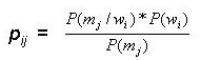
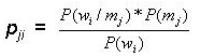
   However, with the same set of words and meanings, we can build a M x W matrix of conditional probabilities P(m/w) each element of which represents the conditional probability that given a word w_i we can expect the meaning m_j. The generic element of this matrix p_ji is given by the formula (2):

   (2)

   A speaker who uses this second conditional probability matrix, in a certain way, adopts the point of view of the hearer, asking itself what is the meaning that the hearer would expect to be associated to the word sent by the speaker. It is the so-called obverter learning introduced by Oliphant and Batali (1997).

1.9

Regarding the structure of the interaction, in this paper the speaker can show the meaning to the hearer with a certain cost, so it will do so only if the hearer does not understand correctly its signal. By communicating the real meaning, the speaker increases the chances that the next encounter among the two players will have a successful outcome. Concerning the cognitive process of the agents, an algorithm based on data mining techniques will be proposed, an induction process that allows the agents to develop decision trees through which they can associate a certain meaning to the signal they receive.

1.10

Compared to the existing literature on the argument, this paper not only proposes a new lexicon formation process but considers a much larger population, with 200 agents that are randomly matched in every period, while previous works on the subject consider much smaller populations. Even with this relatively large number of agents, the population reaches perfect coordination with a number of periods that is very low compared to the results that are typically obtained in this kind of models.

Theoretical framework

2.1

In this paper, the social aspect of the model is based on the framework of evolutionary game theory, where in each period every agent is randomly matched with another agent of the population in order to play a particular game. From the interaction each player gets a pay-off specified by the game's pay-off matrix. While in the classical evolutionary game theory each agent is associated with a strategy and its reproductive success depends on its cumulated pay-off, in this paper every agent can choose a strategy among a set of strategies and, so, every agent has to decide, in each match, what to do.

2.2

In a game, the best action for a player depends on the action of its partner. So, the problem an agent faces in each match is to forecast somehow its partner's move. The agent's forecast depends on the information it could get from the previous games (its experience), on the information it can get from the current game and on the decision process through which the agent computes this information.

2.3

One example is the decision process called fictitious play: the agent is endowed with a vector of frequency indexes (one for every strategy) that it updates after every match according to the strategy the agent's opponent played. This vector summarizes the historic information about the choices the agent's opponents made in the past matches, giving the agent a probability distribution over its opponent's choice. On the basis of this information, the agent can choose the strategy with the best expected pay-off.

2.4

Generally speaking, every model where the agents have to make a decision among a set of actions has to include assumptions about the information the agent can gather and the cognitive mechanism, or algorithm, through which the agent processes the information at its disposal.

2.5

The cognitive aspect of the model presented in this paper is based on the Fast and Frugal Heuristics Theory (FFHT) introduced by Gigerenzer and Goldstein (1996). In the decision process model suggested by the FFHT, the agent classifies a situation by means of a mental model built from its experience. The main point of the FFHT is that the agents classify the situations in a lexicographical way, that is, considering sequentially a certain number of attributes on the basis of their relevance in discriminating different situations. The mental model through which the agent classifies the situations can be represented by a decision tree where each node is an attribute and the branches that depart from it represent the possible attributes' states. For instance, considering situations characterized by three attributes (Attribute 0, Attribute 1 and Attribute 2) that can be in each period in one of two states (0 or 1) and an agent that is endowed with two possible actions (A or B), we can have the mental model illustrated in Figure 1.

2.6

The numbers in the ovals are the attributes' indexes, the numbers besides the arrows are the possible attributes' values and the letters in the rectangular shapes, the tree's leaves, are the agent's possible actions. The decision tree in Figure 1 shows that the agent looks first at Attribute 2's value and, if this value is 0, its decision process does not proceed further: it chooses action B. If, however, the value of Attribute 2 is 1, the agent considers Attribute 0's value: if it is 0 it will choose action A, otherwise it will consider the last attribute, Attribute 1. For example, given the mental model shown in Figure 1, facing the situation 011 the agent will choose action A. The mental model allows the agent to associate an action to every situation it can encounter.

2.7

The FFHT, however, does not tell us anything about the process through which the agent builds its mental model. Indeed, the purpose of the authors of this theory is to show that this lexicographic decision process is in many cases as successful as other classical classificatory techniques, such as the multiple linear regression.

2.8

In this paper I have tried to suggest a model of decision tree's formation and evolution based on an inductive process that the agents perform on the database of their experiences. In particular, the model of the induction process presented here is based on data mining techniques.

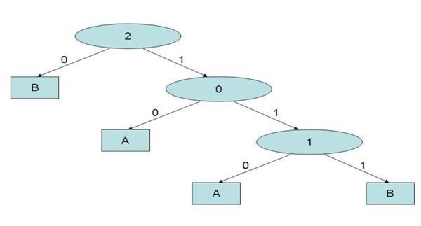
Figure 1. A mental model

Data Mining

3.1

Data mining techniques are used to look for regularity or patterns in a database composed by vectors of historical values of a certain number of variables and have been used in this paper to develop the model of the induction process that allows the agents to detect regularities, and so to make generalizations, from their experiences' database.

3.2

Data mining techniques differ from other forecasting techniques, like the multiple linear regression, for two characteristics that make these techniques particularly suitable for the construction of a model of the decision making process in this paper's context. First of all, the variables that compose the database on which the data mining techniques are applied are discrete. Also when the variables are continuous, they have to be transformed in discrete variables through the introduction of appropriate ranges. In the context of this paper, where social interaction takes the form of a game, this is an advantage because in a game, typically, the agent's strategy space is discrete.

3.3

Second, and most important, the regression techniques are compensatory, that is, all the variables are considered without any particular order: what we do is simply to add all the variables' values after having multiplied them by appropriate weights. The data mining techniques, instead, are lexicographic: they classify the different variables according to their relevance in the classification process. Indeed, while the output of a regression analysis is a linear equation, the outcome of the data mining analysis can be represented as a decision tree that orders hierarchically the independent variables from the most to the least relevant, with leaves that represent the outcome of the decision process.

3.4

For example, we can consider the database shown in Figure 2.

Figure 2: A generic database
Var. 1	Var. 2	Var. 3	Var. 4	Dep. Var.
0	0	1	0	0
0	0	1	1	1
0	1	0	0	0
...	...	....	....	...
1	0	1	1	1
1	1	0	0	0
1	1	0	1	2
....	....	....	....	...
2	1	1	1	0
2	0	1	0	0
2	0	0	1	2

3.5

This is a database composed by the values of five binary variables, four independent variables and one dependent variable. Each line of the database represents an instance: the first line, for example, represents an instance where Var. 1 is in the state 0, Var. 2 is in the state 0, Var. 3 is in the state 1 and Var. 4 is in the state 0, while the dependent variable is in the state 0. We can see that all the variables have discrete values: Var. 1 can be in the states 0, 1 or 2, Var. 2 can be in the states 0 or 1 and so on. What we want to know is the state of the dependent variable given the states of the four independent variables.

3.6

By applying the regression techniques, the outcome will be a linear equation in the following general form:

Dep. Var. = W1*Var. 1 + W2*Var. 2 + W3*Var. 3 + W4*Var. 4

where W1, W2, W3 and W4 are the weights of the independent variables.

3.7

The purpose of the application of data mining is, instead, to make the structure, or the logic, that lies behind this list of instances emerge. In other words, through the data mining techniques we can extract knowledge from the database, discovering not just statistical relations among variables, but the theoretical or logic structure of the database. Relatively to the database represented in Figure 2, these techniques would allow us to obtain, for example, the outcome shown in Figure 3.

3.8

Figure 3 shows a tree like the decision tree introduced as a model of the agent's mental model by the FFHT. We can see that the most important variable to forecast the value of the dependent variable is Var. 4: if it has the value 0, we don't need to consider any other variable because we can already forecast that the dependent variable will be in the state 0. If Var. 4 has the value of 1, instead, we need to consider also Var. 3 : if it has the value 0 we forecast that the dependent variable will have the value 2, otherwise we have to consider Var. 2. From this tree we can see that Var. 1 has no impact on the value of the dependent variable.

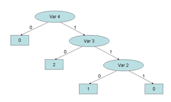
Figure 3. The decision tree resulting from data mining analysis performed on the database shown in Figure 2

3.9

While in the case of multiple linear regression we commonly speak of forecasting techniques, data mining is usually considered a classificatory technique. However, this distinction depends on the nature of the variables typically considered by the two techniques. In general, if the independent variables and the dependent variable are variables that belong to different periods we will normally talk of forecasting analysis. One example could be the analysis of a database consisting of independent variables that describe the meteorological conditions of a given day and the dependent variable representing the presence or absence of rain the following day. If, instead, the variables that compose the database do not have a temporal dimension we then talk of classificatory analysis. One example would be the analysis of a database where the independent variables are the attributes of a tree's leaf (dimension, shape, colour, etc.) and the dependent variable is the tree's kind.

3.10

To summarize, data mining techniques allows us to develop the decision tree by the means of which, according to the FFHT, the agent analyses the situations it has to react to. But while the FFHT does not tell us how to build this decision tree, data mining gives us the algorithm we need to build it from the database of the agent's experiences. In this way, the agent's decision tree becomes the product of two linked processes: the cognitive process, internal to the agent, and the social and historic process, represented by the agents' interactions with each other. In fact, here we have a feed-back process: the interactions among the agents produce their experiences; these experiences, through the induction process, produce the agents' mental models; the agents' mental models determine the agents' behaviour and, thus, the experiences they undergo.

3.11

Now, an example is presented to describe the data mining technique used in the model presented in this paper. We consider the database of Figure 4. It is formed by three independent variables ( I1, I2, I3 ) and one dependent variable (V), whose values have been stored for 20 periods. The first and the third independent variables and the dependent variable are binary variables: they can have values 0 or 1. The second independent variable can have the values 0, 1 or 2.

3.12

The first task of data mining is to find out the first independent variable of the decision tree. In order to do so, we have to compute the average information value of each independent variable.

3.13

According to the information theory, the information value of a database is 1 minus the entropy of the database. The database entropy is defined as the number of bits required to specify the class of an instance given that it belongs to the database. The entropy value can go from 0, if the information that an instance belongs to the database is all we need to classify the instance, to 1, if the fact that the instance belongs to the database does not gives us any useful information about its class.

3.14

If we call N the total number of instances in a database composed by an dependent variable that can have r values, n₀ the number of instances whose value is 0 and n₁ the number of instances whose value is 1, the entropy E of a database is given by (3):

E = - ( n 0/ N)log r ( n 0/ N) - ( n 1/ N)log r ( n 1/ N)

(3)

For example, if we look at the dependent variable column of the database of Figure 10, we see that there are 8 instances that have value 0 and 12 instances that have value 1. The entropy of this database is given by:

E(D) = - (8/20)log2 (8/20) - (12/20) log2 (12/20)

3.15

Therefore, the entropy of the database is 0.971. It represents the additional number of bits we need in order to classify an instance given that it belongs to the database. The information value of the database info(D) is:

info(D) = 1- 0.971 = 0.029

3.16

If the database was composed by an equal number of 0's and 1's, the entropy would be 1 and the information value of the database 0: the fact that an instance belongs to the database, in this case, would not give us any useful information regarding its class. Conversely, if the database was composed, for example, by twenty 1s, the database's entropy would be 0 and the information value 1. The fact that an instance belongs to the database would give us all the information we need to classify the instance: it has to belong necessarily to class 1.

Figure 4 A database
	I1	I2	I3	V
1	0	2	1	1
2	0	1	0	1
3	0	2	0	1
4	1	2	1	0
5	0	1	1	0
6	1	0	1	0
7	1	2	1	1
8	0	0	0	1
9	0	0	0	0
10	1	0	1	1
11	1	1	0	0
12	1	1	1	0
13	1	1	0	0
14	1	2	0	1
15	0	1	0	1
16	1	1	1	0
17	0	1	0	1
18	0	1	0	1
19	0	2	0	1
20	1	0	1	1

3.17

With these basic information theory concepts we are now able to compute the average information value of each independent variable. For each independent variable we can identify as many subsets of the dependent variable vector as the values the variable can have. For example, let's consider variable I1. It can have value 0 or value 1, so we can build two subsets from the initial database of Figure 4: the subsets of instances where I1 is 0, that we call V(I1=0), and the subset of instances where I1 is 1, V(I1=1) (Figure 5 and Figure 6). Now we can calculate the entropy of each database.

E[V(I1=0)] = - (2/10)log2 (2/10) - (8/10) log2 (8/10) = 0.722 E[V(I1=1)] = - (6/10)log2 (6/10) - (4/10) log2 (4/10) = 0.971

Figure 5: Figure 5: V(I1=0)
V(I1=0)
1
1
1
0
1
0
1
1
1
1

Figure 6: Figure 6: V(I1=1)
V(I1=1)
0
0
1
1
0
0
0
1
0
1

3.18

Being the dimension of both the subsets 10, the average entropy of variable I1, that we call E(I1), is:

E(I1) = (10/20) * 0.722 + (10/20) * 0.971 = 0.846

3.19

For the information theory, it means that if we know the value variable I1 has in a particular instance, to correctly classify that instance we need, on average, 0.846 additional bits. The average information value of I1, info(I1), is, consequently:

info(I1) = 1- 0.846 = 0.154

3.20

We now repeat the procedure for the second independent variable I2. First, we have to build the subsets of the original database. Being I2 a variable that can have three values, we will identify three subsets, that are represented below (Figure 7, Fig 8 and Figure 9).

3.21

The first database contains the class of instances where I2 has value 0, the second database contains the class of instances where I2 has value 1 and the third database contains the class of instances where I2 has value 2. We calculate the databases' entropies:

E[V(I2=0)] = - (2/5)log2 (2/5) - (3/5) log2 (3/5) = 0.971 E[V(I2=1)] = - (5/9)log2 (5/9) - (4/9) log2 (4/9) = 0.994 E[V(I2=2)] = - (1/6)log2 (1/6) - (5/6) log2 (5/6) = 0.649

Figure 7: V(I2=0)
V(I2=0)
0
1
0
1
1

Figure 8: V(I2=1)
V(I2=1)
1
0
0
0
0
1
0
1
1

Figure 9: V(I2=2)
V(I2=2)
1
1
0
1
1
1

3.22

Given the databases' dimensions (respectively 5, 9 and 6), the average entropy of variable I2 is:

E(I2) = (5/20) * 0.971 + (9/20) * 0.994 + (6/20) * 0.649 = 0.885

3.23

The average information value of I2 is:

info(I2) = 1- 0.885 = 0.115

3.24

Following the same procedure, we find the average information value of variable I3:

info(I3) = 1- 0.912 = 0.088

3.25

So, the most informative variable, that is the variable with the highest average information value, is variable I1 and so this is the first variable of the decision tree. Being variable I1 a binary variable, the root of the decision tree will have two branches, one for each possible value of variable I1 (Figure 10).

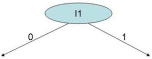
Figure 10. First node

3.26

The next step is to find out the variable with the highest average information value for each branch, excluding variable I1 that has already been chosen as root of the decision tree. This means building a database for each branch: a database of instances where I1 has value 0 and a database where I1 has value 1 (Figure 11 and Figure 12).

Figure 11: D(I1 = 0)
	I2	I3	V
1	2	1	1
2	1	0	1
3	2	0	1
4	1	1	0
5	0	0	1
6	0	0	0
7	1	0	1
8	1	0	1
9	1	0	1
10	2	0	1

Figure 12: D(I1 = 1)
	I2	I3	V
1	2	1	0
2	0	1	0
3	2	1	1
4	0	1	1
5	1	0	0
6	1	1	0
7	1	0	0
8	2	0	1
9	1	1	0
10	0	1	1

3.27

For each of them we will calculate the average information value of I2 and I3 and we will choose for each node the variable with the highest average information value, determining in this way the two second best variables of the decision tree.

The Model

4.1

The model presented in this paper is an agent-based computational model and, as such, it has to be described at two different levels: the agent's level and the population level. At the first level we have to describe the agent, with its characteristics and skills, while, at the second level, we have to describe the way the agents who compose a population interact with each other.

4.2

In this model, each agent is endowed with a string of three attributes, or symbols. Each of them can be freely set by the agent in state A or B. The agents, therefore, can set the state of the whole string to one of eight possible states (AAA, AAB, etc.). Moreover, each agent can see the state of the string of other agents with whom it interacts, so the string becomes a way the agents can send messages to their partners in each game.

4.3

The agents are endowed with a memory where they store the messages observed in the past. The size of the memory, that is the number of instances in the agent's database, is a parameter of the model. New experiences enter the agent's database with a FIFO system: when the agent's memory is full the oldest experience in the database is discarded to make room for the most recent experience.

4.4

The agents are endowed with the cognitive capacity to perform data mining algorithms on their memory's database, a capacity that allows them to draw deductive inferences from their experiences. To see the use the agents make of these gathering, storing and processing skills, we have to describe the second level of the model, the social process of reiterate interactions among the agents of the population.

4.5

The game can be defined as a common-interest signaling game: one of the two players, Player S (the sender) draws a number from an urn containing the eight integers from 0 to 7 and, after having seen the number, sends a message to its partner, Player R (the receiver). The information about which number has been drawn by Player S is not available to Player R, who can observe only the message sent to it by Player S. Player S can send one of the eight possible messages by combining the three binary attributes it is endowed with. The fact that one of the players sends a message to the other player makes the game a signaling game.

4.6

The pay-off the two players get from the interaction depends on the capacity of Player R to guess correctly which number has been drawn by Player S: if Player R guesses correctly both players get a pay-off of 1, while if it guesses wrongly both get a pay-off of 0. The fact that it is in the interest of both players that Player R guesses correctly makes the game a common-interest game.

4.7

At the end of the game, if Player R's guess is wrong, Player S discloses the number it meant with its message. This information exchange does not increase the players' pay-off in the current game but, given the positive likelihood that the two players will meet again in subsequent games, it is in the interest of Player S to disclose this information in order to increase the chance that the two players will coordinate in the future. Therefore, we can say that in the game proposed in this paper, the sender has the role of the teacher and the receiver the role of the learner.

4.8

To summarize, in each match Player S draws a number and sends a message to Player R, who observes the message and guesses which number has been drawn by Player S. After Player R's guess, if the guess is wrong Player S will show its partner which number it actually meant by its message.

4.9

At the beginning of the simulation there is no socially shared convention that associates a number to a message, so the only thing Player S can do is to send Player R a message chosen randomly among the eight possible messages. At the same time, Player R can only make a random guess among the eight integers Player S can draw. Of course at the beginning Player R's guesses will be right, on average, one every eight matches.

4.10

After every match, the players will update their database with the information they could get from the interaction: a message and a number associated to the message. Both players will memorize the message sent by Player S with the number it drew. In the database of the two players, each one of the three attributes of the message represent an independent variable and the number associated to the message represents the dependent variable. For instance, the database of a generic agent, who we call agent Tom, could be the one shown in Figure 13.

4.11

The last row tells us the input coming from agent Tom's last experience. In this last game agent Tom could be the sender or the receiver. In the first case, 2 is the number it drew and AAB is the message it sent to its partner. If agent Tom was, instead, the receiver, then 2 is the number drew by its partner and AAB is the message it was sent by Player S.

4.12

In every period, new couples are randomly formed, so that in every game each agent is likely to meet a different agent from the one it met in the previous game. Moreover, in every game the roles are randomly assigned, so that each player will find itself to be, on average, the sender in half of the games and receiver in the other half.

Figure 13: Agent Tom experiences' database
Symbol 0	Symbol 1	Symbol 2	Number
A	B	A	5
B	A	A	0
B	B	A	7
...	....	....	...
B	A	B	2
B	B	A	6
A	A	A	6
....	....	....	...
A	B	B	4
A	B	B	3
A	A	B	2

4.13

As said before, for the first matches the players will choose random messages and will make random guesses. However, after a certain number of matches, a number that is a parameter of the model and that in the simulations presented below has been set equal to the agent's memory size, the agents will begin to draw inductive inferences from their experiences. These inferences will allow each player to develop expectations regarding the meaning a particular message has for the other players: Player S will use these expectations to send the right message given the number it has drawn and Player R will use them to guess the right number given the message it has been sent. In other words, Player S will send the message that it believes Player R will associate to the number Player S has drawn, and Player R will choose the number it believes Player S associates to the message Player S sent.

4.14

The tool the agents use to draw inductive inferences from the database of their experiences is the data mining technique described above. So, their expectations about other agents' messages meaning will take the form of a decision tree. The agent's expectations will be referred to as the agent's mental model. For example, let's consider a match with two players having developed the mental models shown below in Figure 14 and Figure 15.

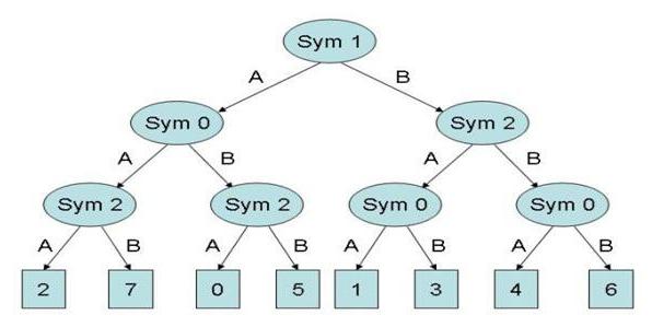
Figure 14. Player S Mental Model

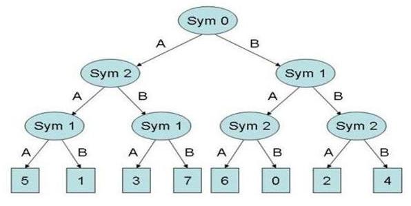
Figure 15. Player R Mental Model

4.15

Player S draws the number 7. Its mental model (Figure 14) tells it that the message the other player is likely to associate to the number 7 is AAB, because the number 7 is at the end of the path where the second symbol of the message (Sym 1) is A, the first symbol (Sym 0) is A and the last symbol (Sym 2) is B. So, it sends the message AAB to Player R. Player R gets this message and reads it through its mental model (Figure 15). It tells the agent that with the message AAB the other player probably meant the number 3 because this is the number we find following the path (Sym0=A)-(Sym2=B)-(Sym1=A). Therefore, the number 3 is its guess. In this match, Player B's guess is wrong so both players get a pay-off of 0. At this point, Player S communicate to Player R the right number and both players will update their database with this last experience, memorizing the message AAB associated to the number 7. The updated database will cause both players to draw new inductive inferences and, thus, to change their mental model.

4.16

The number of experiences after which the mental model gets updated, that we will call the mental model updating lag, represents the third parameter of the model: its value can go from 1, if the agent makes new inductive inferences after every match, to the agent's memory size.

4.17

What has been described above is a feed-back process where the experiences the agents make determine their mental models and their mental models, in turn, determine their behaviour and, so, their experiences. The question we try to answer with the simulation that will be presented below is: what will be the outcome of this process? Will the population ever reach an equilibrium where the agents' mental models get confirmed by their experiences? That is, will the system develop a socially shared lexicon, a convention where the agents associate the same numbers to the same messages?

Simulation Results

5.1

The aim of the simulations is to show if a population of agents having the cognitive skills specified above will ever develop a common understanding of the messages they can produce, that is, if the agents will develop a socially shared convention that makes them mean the same thing with the same combination of symbols. In this case, the agents will reach a perfect coordination equilibrium, a situation where in every match that takes place in every period, Player R can always guess, by reading the message it gets from Player S, the number drawn by the latter.

5.2

To run the simulations the following parameters are set:

• number of agents: 200
• number of words: 8
• length of memory (periods): 60
• mental model updating lag (periods): 1

5.3

The number of agents who successfully coordinate with their partner is the variable we want to track. Considering a population of 200 agents, this number can vary from 0, when in all the 100 games the players failed to coordinate, to 200, when in all the games the players coordinated successfully. Of course, at the beginning, when all the receivers guess randomly, the value of coordination degree will fluctuate around the value of 25 because in only one every eight games Player R will guess the number Player S actually drew.

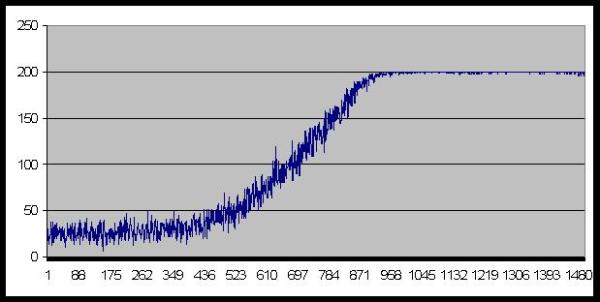
Figure 16. Number of agents who coordinate successfully

5.4

A typical result of the simulations is shown in Figure 16. As the graph shows, after the first stage, lasting approximately 400 periods, the number of agents who coordinate successfully begins a quite rapid growth that ends after about 900 periods, when a social convention gets established that allows a perfect coordination among the agents. The simulation shows that the population as a whole converges quite rapidly towards an equilibrium represented by a situation where the same message means the same thing for all the agents of the population. The emergence of a socially shared lexicon looks like a transition phase.

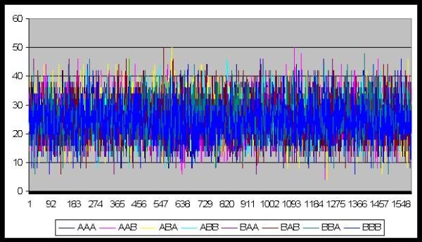
Figure 17. Number of messages chosen

5.5

Regarding the messages chosen by the agents, Figure 17 shows that all the 8 words are chosen statistically with the same frequency. This means that the cognitive process proposed is successful in assigning a word to each number and synonyms do not emerge.

5.6

The following four graphs show the result of simulations run with parameters set at different values, in order to tackle the issue of scalability of the model. The four main parameters we focused on are:

• the number of agents
• the number of words and numbers
• the memory's length
• the mental model updating lag

5.7

The graphs shown in Figure 18, 19, 20 and 21, show the average number of periods that it took to reach the perfect coordination over 10 runs with different parameters values. As we can see from he graph shown in Figure 18, the time it takes to reach equilibrium increases less than proportionally increasing of the number of agents: doubling the population's size from 200 to 400 (+100%) increases the average time to reach the equilibrium from 900 to 1100 (+22%).

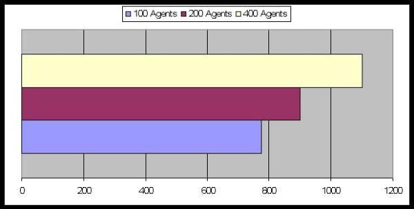
Figure 18. Average Number of Periods to reach equilibrium: the effect of the population's size

5.8

Instead, the graph shown in Figure 19, shows that the complexity of the environment the agents face, that is the number of objects they have to name and the number of words the agents can produce, is a crucial factor for the emerge of a shared lexicon: in fact, doubling the number of words from 8 to 16 increases the number of periods it takes to reach the equilibrium by a factor of 2.7, from 900 to around 2500 periods. This may suggest that the expansion of a population's vocabulary is a process that proceeds by stages: once the agents in the population have succeeded in naming few basic concepts by the means of short set of symbols, they can use these strings of symbols as building blocks to name other, more complex, concepts.

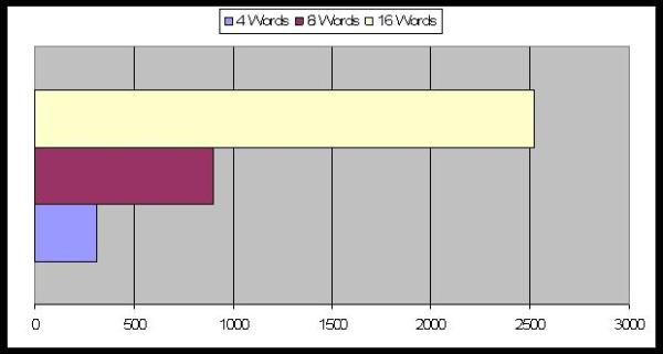
Figure 19. Average Number of Periods to reach equilibrium: the effect of the words' number

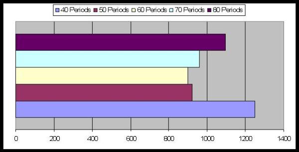
Figure 20. Average Number of Periods to reach equilibrium: the effect of the memory's length

5.9

The graphic of Figure 20, shows the effect of the memory's length on the average time it takes to reach the equilibrium. It shows that there is an optimal length, that in this case is 60, below and above which the average number of periods increases. This may suggest that there is a trade-off between the variability of the mental models, and, so, the variability of the agents' behaviour, and the rigidity of the mental models relatively to out-of-date experiences. In other words, the mental models should be stable enough to constitute a reliable basis for other agents' expectations but should not be so stable not to adapt to new evidence.

5.10

Finally, the graphic of Figure 21 shows the effect of different mental memory updating lags. The graphic shows that the more often the mental models are updated the better for the emergence of the social convention, but the effect is less than proportional.

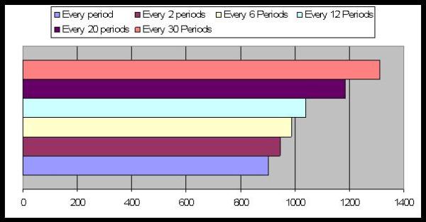
Figure 21. Average Number of Periods to reach equilibrium: the mental model updating lag

Conclusions

6.1

This paper has proposed a model of the process through which different combinations of symbols are assigned a socially shared meaning by a population of agents without any central authority intervention. The simulations have shown that, given certain assumptions about the agents' cognitive skills, a process of iterated bilateral interactions among randomly paired agents leads inevitably to the emergence of a social convention that allows the agents to 'understand' each other. The simulations show that, given the induction process presented in this paper, a social convention can emerge in relatively few periods even with a relatively large population, a result that distinguishes the results of this paper from the results of previous studies on the argument, where the emergence of a shared convention takes a very long time even with few agents.

6.2

Of course, every simulation leads to a different convention. With eight messages available to describe eight objects, there are 40320 different conventions. Which one of them is actually adopted by the population depends on a series of random fluctuations, or historical accidents. However, after a particular convention emerges it is very stable because every agent's behaviour confirms every other agent's expectation. We can say that the feed-back process experiences-expectations-experiences reaches a steady state, or equilibrium, where the expectations produce experiences that confirm the expectations.

6.3

We have to observe that once a convention has emerged, the decision about what message to send and what to respond to a message that has been received does not need to go through all the data mining process that allowed the selection of a particular equilibrium: the agents simply learn to associate a message to a number, in an automatic way.

6.4

This model, not only suggests a possible mechanism for the emergence of the meaning of words, but supports, indirectly, the cognitive process suggested by the FFHT, that is, the lexicographic analysis of input by the means of a decision tree. The model presented in this paper goes a step further because it suggests a possible endogenous process, implemented using data mining techniques, through which the agents' decision trees form and co-evolve on the basis of the agents' experiences.

Acknowledgements

This paper is based on my PhD thesis "The formation of mental models in social contexts: a computational model", the outcome of a three-year research period at the University of Bologna.

I wish to thank my PhD supervisor Prof. Roberto Scazzieri for his constant support during all the stages of the research.

I am grateful to Prof. Nigel Gilbert who, during the three-month research period I spent at the University of Surrey, gave me precious advice that helped me to critically reconsider my work, allowing me to amend some of its weak points.

I wish to thank Prof. Pietro Terna and his PhD students for the invaluable help they gave me regarding the technical aspects of the agent-based simulation.

Appendix

The code has been written in Java and consists of two classes: the agent and the class containing the function main() that we called Society.

The Agent class

import java.util.ArrayList;
import java.util.Random;
public class Agent {
private int Address;
private int Object;
private int Age;
private boolean Forecast;
private boolean DT;
private int[] Word;
private int MemoryLenght;
private int Period;
private int[][] Sym;
private int[] Meaning;
private int Root;
private int[] SnNode;
private int[][] TrNode;
private int[][][] TrNodeLeaf;
private int Guess;
private int numberObjects;
private int wordLenght;
private int numberSymbols;
Random rand = new Random();
private int numAgents;
private int LearningPeriod;
public Agent (int i, int no, int wl, int ns, int p, int m) {
	rand.setSeed(Society.get_Seed()*(i+1));
	Address = i;
	numberObjects = no;
	wordLenght = wl;
	numberSymbols = ns;
	numAgents = p;
	Period = 0;
	MemoryLenght = m;
	LearningPeriod = MemoryLenght-2;
	Root = -1;
	DT = false;
	Sym = new int[wordLenght][MemoryLenght];
	Meaning = new int[MemoryLenght];
	Word = new int[wordLenght];
	SnNode = new int[numberSymbols];
	TrNode = new int[numberSymbols][numberSymbols];
	TrNodeLeaf = new int [numberSymbols][numberSymbols][numberSymbols];
}

public void build_DecisionTree() {
	if ( Period > LearningPeriod && rand.nextDouble() < 0.2 ) {
	DT = true;
	double[][] cs = new double[wordLenght][numberSymbols];
	double[][][] csm = new double[wordLenght][numberSymbols][numberObjects];
	double[] infoVal = new double[wordLenght];
int[][][][] countWord = new int[numberSymbols][numberSymbols][numberSymbols][numberObjects];
	for ( int i = 0; i < numberSymbols; i++ ) {
		for ( int j = 0; j < numberSymbols; j++ ) {
			for ( int y = 0; y < numberSymbols; y++ ) {
					for ( int k = 0; k < numberObjects; k++ ) {
					countWord[i][j][y][k] = 0;
					}}}}
	for ( int j = 0; j < wordLenght; j++ ) {
		infoVal[j] = 0;
		for ( int i = 0; i < numberSymbols; i++ ) {
			cs[j][i] = 0;
				for ( int z = 0; z < numberObjects ; z++ ) {
					csm[j][i][z] = 0;
				}}}
	for ( int j = 0; j < wordLenght; j++ ) {
		for ( int y = 0; y < numberSymbols; y++ ) {
		for ( int i = 0; i < Period ; i++ ) {
			if ( Sym[j][i] == y )
			 cs[j][y] += 1;
			for ( int z = 0; z < numberObjects ; z++ ) {
				if ( Sym[j][i] == y && Meaning[i] == z )
					 csm[j][y][z] += 1;
			}}}}
	for ( int j = 0; j < wordLenght; j++ ) {
		for ( int i = 0; i < numberSymbols; i++ ) {
				for ( int z = 0; z < numberObjects ; z++ ) {
if ( cs[j][i] != 0 && csm[j][i][z] != 0 )
infoVal[j] += 
cs[j][i]*(-1*(csm[j][i][z]/cs[j][i])*Math.log(csm[j][i][z]/cs[j][i]));
			}}}
	double bestIV = infoVal[0];
	for ( int j = 1; j < wordLenght; j++ ) {
		if ( infoVal[j] < bestIV ) { 
			bestIV = infoVal[j];
		}}
	int[] check2 = new int[wordLenght];
	for ( int k = 0; k < wordLenght; k++ ) {
		check2[k] = 0;
	}
	for ( int h = 0; h < wordLenght; h++ ) {
		if ( infoVal[h] == bestIV )
			check2[h] = 1;
	}
	int f;
	do {
		f = rand.nextInt(wordLenght);
	}while (check2[f] == 0);
	Root = f;
	int countSR;
	for ( int q = 0; q < numberSymbols; q++ ) {
		countSR = 0;
		for ( int r = 0; r < Period ; r++ ) {
			if ( Sym[Root][r] == q ) 
				countSR += 1;
		}
	int[][] srSym = new int[wordLenght-1][countSR];
	int[] srMea = new int[countSR];
		for ( int j = 0, y = 0; j < wordLenght-1 && y < wordLenght; ) {
			int p = 0;
			if ( Root == y )
				y += 1;
			for ( int i = 0; i < Period ; i++ ) {
				if ( Sym[Root][i] == q ) {
				srSym[j][p] = Sym[y][i];
				srMea[p] = Meaning[i];
				p += 1;
				}
				}
			j += 1;
			y += 1;
		}
		double[][] sr_cs = new double[wordLenght-1][numberSymbols];
		double[][][] sr_csm = 
            new double[wordLenght-1][numberSymbols][numberObjects];
		double[] sr_infoVal = new double[wordLenght-1];
				for ( int j = 0; j < wordLenght-1; j++ ) {
					sr_infoVal[j] = 0;
					for ( int i = 0; i < numberSymbols; i++ ) {
						sr_cs[j][i] = 0;
					for ( int z = 0; z < numberObjects ; z++ ) {
						sr_csm[j][i][z] = 0;
							}}}
				for ( int j = 0; j < wordLenght-1; j++ ) {
					for ( int y = 0; y < numberSymbols; y++ ) {
					for ( int i = 0; i < countSR ; i++ ) {
						if ( srSym[j][i] == y )
							sr_cs[j][y] += 1;
						for ( int z = 0; z < numberObjects ; z++ ) {
							if ( srSym[j][i] == y && srMea[i] == z )
								sr_csm[j][y][z] += 1;
						}}}}
				for ( int j = 0; j < wordLenght-1; j++ ) {
					for ( int i = 0; i < numberSymbols; i++ ) {
				      for ( int z = 0; z < numberObjects ; z++ ) {
			if ( sr_cs[j][i] != 0 && sr_csm[j][i][z] != 0 )
 sr_infoVal[j] += sr_cs[j][i]*
(-1*(sr_csm[j][i][z]/sr_cs[j][i])*Math.log(sr_csm[j][i][z]/sr_cs[j][i]));
						}}}
				double sr_bestIV = sr_infoVal[0];
				for ( int j = 1; j < wordLenght-1; j++ ) {
					if ( sr_infoVal[j] < sr_bestIV )  
						sr_bestIV = sr_infoVal[j];
					}
				for ( int k = 0; k < wordLenght-1; k++ ) {
					check2[k] = 0;
					}
				for ( int h = 0; h < wordLenght-1; h++ ) {
					if ( sr_infoVal[h] == sr_bestIV )
						check2[h] = 1;
					}
				do {
					f = rand.nextInt(wordLenght-1);
				} while (check2[f] == 0);
				SnNode[q] = f;
				if ( Root == 0 ) {
					SnNode[q] += 1;
				}
				if ( Root == 1) {
					if ( SnNode[q] > 0 )
					SnNode[q] += 1;
				}		
			     for ( int k = 0; k < numberSymbols; k++ ) {
			     for ( int i = 0; i < wordLenght; i++ ) {
				if ( i != Root && i != SnNode[q] )
					TrNode[q][k] = i;
								}
				for ( int v = 0; v < numberSymbols; v++ ) {
				for ( int h = 0; h < numberObjects; h++ ) {
			      for ( int t = 0; t < Period; t++ ) {
	if ( Sym[Root][t] == q && Sym[SnNode[q]][t] == k && 
        Sym[TrNode[q][k]][t] == v && Meaning[t] == h )
           countWord[q][k][v][h] += 1;
		}
      int bestMeaning = 0;
	for ( int h = 0; h < numberObjects; h++ ) {
	if ( countWord[q][k][v][h] > bestMeaning )
	bestMeaning = countWord[q][k][v][h];
				}
	int[] countTNL = new int[numberObjects];
for ( int h = 0; h < numberObjects; h++ ) {
countTNL[h] = 0;
}
for ( int h = 0; h < numberObjects; h++ ) {
	if ( countWord[q][k][v][h] == bestMeaning )
	countTNL[h] = 1;
}
	do {
      f = rand.nextInt(numberObjects);
	}while(countTNL[f] == 0 );
	TrNodeLeaf[q][k][v] = f;
}}}}}

public void update_DataSet() {
	for ( int j = 0; j < wordLenght; j++ ) {
	for ( int i = Period-1; i > -1 ; i-- ) {
		Sym[j][i+1] = Sym[j][i];
		}
	}
	for ( int i = Period-1; i > -1 ; i-- ) {
		Meaning[i+1] = Meaning[i];
		}
	for ( int j = 0; j < wordLenght; j++ ) {
	Sym[j][0] = Word[j];
	}
	Meaning[0] = Object;
	if ( Period < MemoryLenght-1 )
		Period += 1;
}

public void think_Word() {
	if ( DT == true ) {
		int c = 0;
		int[][] word = new int[numberSymbols*numberSymbols*numberSymbols][wordLenght];
		for ( int i = 0; i < numberSymbols; i++ ) {
			for ( int j = 0; j < numberSymbols; j++ ) {
					for ( int k = 0; k < numberSymbols; k++ ) {
		        if ( TrNodeLeaf[i][j][k] == Object ) {
		        	word[c][Root] = i;
		        	word[c][SnNode[i]] = j;
		        	word[c][TrNode[i][j]] = k;
		        	c += 1;
		        }}}}
		if ( c != 0 ) {
		int f = rand.nextInt(c);
		for ( int j = 0; j < wordLenght; j++ ) {
			Word[j] = word[f][j];
			}	}
		else {
			for ( int j = 0; j < wordLenght; j++ ) {
				Word[j] = rand.nextInt(numberSymbols);;
				}}}
		else {
			for ( int j = 0; j < wordLenght; j++ ) {
				Word[j] = rand.nextInt(numberSymbols);;
				}}}

public void draw_Object() {
	Object = rand.nextInt(numberObjects);
}

public void guess_Object() {
	if ( DT == true ) {
		int a = Word[Root];
		int b = Word[SnNode[a]];
		int c = Word[TrNode[a][b]];
		Guess = TrNodeLeaf[a][b][c];
		if (  Guess == -1 )
		Guess = rand.nextInt(numberObjects);
		}
		else {
			Guess = rand.nextInt(numberObjects);
		}
	if ( Guess == Object )
		Forecast = true;
	else
		Forecast = false;
}


public void get_Guess(Agent a) {
	Guess = a.guess();
	if ( Guess == Object )
		Forecast = true;
	else
		Forecast = false;
}

private int guess() {
	return Guess;
}

public int get_Object() {
	return Object;
}

public int[] get_Sig() {
	return Word;
	
}

public void get_Message(Agent a) {
	Object = a.get_Object();
	int[] word = a.get_Sig();
	for ( int j = 0; j < wordLenght; j++ ) {
		Word[j] = word[j];
		}
}

public boolean get_Forecast() {
	return Forecast;
}

public int get_Word0() {
	return Word[0];
}

public int get_Word1() {
	return Word[1];
}

public int get_Word2() {
	return Word[2];
}

}

The Society class

import java.util.LinkedList;
import java.util.Random;
public class Society {
	private static final long Seed = 918273;
	private static int numAgents = 200;
	private static int Memory = 60;
	private static int numberObjects = 8;
	private static int wordLenght = 3;
	private static int numberSymbols = 2;
	private static int TotalPayOff = 0;
	private static int Time = -1;
	static java.util.List<number> urn;
	static Random rand = new Random();
	public static void main(String[] args) {
		rand.setSeed(Seed);
		urn = new LinkedList<number>();
		Agent[] agent = new Agent[numAgents];
		for ( int i = 0; i < numAgents; i++ ) {
			agent[i] = new Agent(i, numberObjects, wordLenght,    numberSymbols, numAgents, Memory);
		}
		for (int t = 0; t < 2000; t++) {
		for (int i = 0; i < numAgents; i++ ) {
			urn.add(new Number(i));
			}
		for (int i = 0; i < numAgents/2; i++ ) {
			int f;
			int r;
			Number n;
			f = rand.nextInt(urn.size());
			n = urn.get(f);
			r = n.draw_Number();
			urn.remove(f);
			Agent a = agent[r];
			f = rand.nextInt(urn.size());
			n = urn.get(f);
			r = n.draw_Number();
			urn.remove(f);
			Agent b = agent[r];
			a.build_DecisionTree();
			b.build_DecisionTree();
			a.draw_Object();
			a.think_Word();
			b.get_Message(a);
			b.guess_Object();
			a.get_Guess(b);
			a.update_DataSet();
			b.update_DataSet();
		}
		int tpo = 0;
		for (int i = 0; i < numAgents; i++ ) {
			Agent a = agent[i];
			if ( a.get_Forecast() == true ) 
				tpo += 1;
		}
		}
	}
	public static long get_Seed() {
		return Seed;
	}
	public static int get_Time() {
		return Time;
	}
}

References

GIGERENZER, G., and Goldstain, D. G. (1996) "Reasoning the Fast and Frugal Way: Models of Bounded Rationality" Psychological Review: 103, 650-669.

OLIPHANT, M. (1999) "The Learning Barrier: Moving from Innate to Learned Systems of Communication" Adaptive Behaviour: 7, 371-384. OLIPHANT, M. and Batali, J. (1997) "Learning and the Emergence of Coordinated Communication" Centre for Research on Language Newsletter, 11(1).

SMITH, A. D. M. (2001) "Establishing Communication Systems without Explicit Meaning Transmission" Proceedings of the 6th European Conference on Artificial Life. Eds. J. Kelemen and P. Sosik. Berlin: Springer-Verlag.

STEELS, L. (1996) "Emergent Adaptive Lexicons" From Animals to Animats 4: Proceedings of the Fourth International Conference On Simulating Adaptive Behaviour. Ed. P. Maes. Cambridge, Mass.: MIT Press.

STEELS, L. and Kaplan, F. (2002) "Bootstrapping Grounded Word Semantics" Linguistic Evolution through Language Acquisition: Formal and Computational Models. Ed. T. Briscoe. Cambridge: Cambridge University Press.

STEELS, L. and Vogt P. (1997) "Grounding Adaptive Language Games in Robotic Agents" Proceedings of the Fourth European Conference on Artificial Life. Eds. C. Husbands and I. Harvey. Cambridge, Mass.: MIT Press.

VOGT, P. (2001) "The Impact of Non-Verbal Communication on Lexicon Formation" Proceedings of the 13th Belgian/Netherlands Artificial Intelligence Conference. Eds. B. Kröse, M. De Rijke, G. Schreiber and M. Van Someren.

Vogt, P. (2002) "The Physical Symbol Grounding Problem" Cognitive Systems Research, 3(3): 429-457.

VOGT, P. and Coumans, H. (2003) "Investigating Social Interaction Strategies for Bootstrapping Lexicon Development" Journal of Artificial Societies and Social Simulation, 6(1)4 https://www.jasss.org/6/1/4.html.

YANCO, H. and Stein, L. (1993) "An Adaptive Communication Protocol for Cooperating Mobile Robots" From Animals to Animats 2:Proceedings of the Second International Conference On Simulating Adaptive Behaviour. Eds. J. A. Meyer, H. L. Roitblat and S. Wilson. Cambridge, Mass.: MIT Press.

Return to Contents of this issue

© Copyright Journal of Artificial Societies and Social Simulation, [2008]