Sylvie Huet, Margaret Edwards and Guillaume Deffuant (2007)

Taking into Account the Variations of Neighbourhood Sizes in the Mean-Field Approximation of the Threshold Model on a Random Network

Journal of Artificial Societies and Social Simulation vol. 10, no. 1
<https://www.jasss.org/10/1/10.html>

For information about citing this article, click here

Received: 30-Jun-2006    Accepted: 27-Sep-2006    Published: 31-Jan-2007

Abstract

We compare the individual-based "threshold model" of innovation diffusion in the version which has been studied by Young (1998), with an aggregate model we derived from it. This model allows us to formalise and test hypotheses on the influence of individual characteristics upon global evolution. The classical threshold model supposes that an individual adopts a behaviour according to a trade-off between a social pressure and a personal interest. Our study considers only the case where all have the same threshold. We present an aggregated model, which takes into account variations of the neighbourhood sizes, whereas previous work assumed this size fixed (Edwards et al. 2003a). The comparison between the aggregated models (the first one assuming a neighbourhood size and the second one, a variable one) points out an improvement of the approximation in most of the value of parameter space. This proves that the average degree of connectivity (first aggregated model) is not sufficient for characterising the evolution, and that the node degree variability has an impact on the diffusion dynamics. Remaining differences between both models give us some clues about the specific ability of individual-based model to maintain a minority behaviour which becomes a majority by an addition of stochastic effects.

Keywords:

Aggregate; Individual-Based Model; Innovation Diffusion; Mean Field Approximation; Model Comparison; Social Network Effect

Introduction

1.1

Individual-based models are more and more commonly used in ecological modelling (Grimm 1999), or to model social and economical processes (Axelrod 1995;Ellison 1993;Epstein and Axtell 1996;Gilbert and Troitzsch 1999). This work aims at studying the interest of an individual based model compared to an aggregated one. In both cases, we are interested in aggregated variables but the aggregated modelling requires lower computer capacity and time. Therefore, it is interesting to identify the conditions in which an individual based model can be replaced by its aggregated approximation. Recent studies have sought to compare individual-based to aggregate models. De Angelis and Gross (1992) study the influence of transforming continuous variables into discrete distributions in models of ecological dynamics; Picard and Franc (2001) show that space-dependent individual based models and aggregated models (regarding either spatial influence or description of the population) of forest dynamics lead to different results. Fahse et al. (1998) and Duboz et al. (2003) use individual-based models to extract parameters for population-level dynamics.

1.2

This work follows the one presented in Edwards et al. ( 2003a; 2003b) in which an individual based model of innovation diffusion (Valente 1995; Morris 1997) studied by Blume (1993; 1995) and Young (1998; 1999) is aggregated following the principles of sociodynamics (Weidlich 2000; 2002). This model represents individuals who choose between two behaviours (A or B) according to a utility function based on a social benefit (depending on the behaviour of their neighbours and a payoff related to each behaviour) and an individual benefit. Following Blume and Young, we consider that the individual benefit is the same for all the individuals, which allows us to focalise our study on the role of social influence in the dynamics. For convenience we put this individual benefit to zero. The choice is randomised by a Gibbs function with a given temperature (Kirkpatrick, Gelatt and Vecchi 1983).

1.3

Edwards et al. approximate the individual based threshold model on a random network by an aggregate model assuming a network with a fixed number of neighbours for each individual (number of links at each node of the graph). This strong approximation yields pretty good results. The asymptotic behaviours of the two models are identical and can be of two kinds: 0% of A behaviour and 100% of A behaviour. Both models have a bifurcation: following the temperature of the Gibbs function, there can be either one or two possible final attractors. The convergence towards one or the other is linked to the initial percentage in A behaviours. The position and shape of this bifurcation zone depend essentially on the randomness of the individual decision function (temperature of the Gibbs function), on the payoff of A and the mean number of neighbours for an individual for the rest.

1.4

However, we could observe that two types of differences between the individual based model and its aggregated approximation persisted:

• under some conditions the models can exhibit different limits of attraction basins, in terms of initial proportion of A. Therefore, the aggregated model can fail at predicting correctly the threshold value of A behaviours leading to a change of the final state for the IBM;
• In some cases the final state of the individual based model takes an intermediate value between the possible final states predicted by the aggregated model: 0% and 100% of A. Moreover, for some initial conditions, when observing the individual simulations, this value of the final state appears to vary from one run to the other, leading to a bimodal distribution of final states. The aggregated approximation with a fixed neighbourhood size never shows such a behaviour.

1.5

We call the first type of difference — on which we will concentrate — "strong difference" because the final states of respectively the individual-based model and the aggregated models are located on opposite attractors (corresponding respectively to 0% of behaviours A and 100% of behaviours A). We will show that this strong difference is related to the fixed neighbourhood size simplification. Indeed, when the neighbourhood has a strong impact on the decision function, differences between the models can appear.

1.6

To improve the approximation, we propose an extended version of the aggregated model in which we used a Poisson distribution to approximate the variable neighbourhood size in a random network.

Aggregating an individual based threshold model on a random network

The individual based model of innovation diffusion

2.1

The threshold model is initially inspired from the sociology of innovation diffusion (Granovetter 1978). Its principle is that the decision of an individual to change its behaviour relies on a trade-off between a social pressure (considering the behaviour of its neighbours), and an intrinsic, personal interest. Focalising on the influence of social interaction, Blume and Young have only considered the case where the personal interest is zero for all. We do the same here, and we consider the stochastic version of the decision model, which is introduced by Luce (1959) and uses a Gibbs function. We recall hereafter the main features of the model.

2.2

We consider N individuals, having the choice between two behaviours: A and B. N is constant over time. The individuals are connected to each other through a random graph (social network): we choose a priori a number of links for the whole population, and pick pairs of individuals at random to define the links. Afterward, each individual e has a neighbourhood V(e) (individual social network), which is the set of individuals he is connected with through the graph. The social network is therefore characterised by an average number of links v for an individual (average neighbourhood size).

2.3

To take an example, let's consider a village, the watering practices of which we would like to follow; A represents scarce watering and B generous watering. Individuals choose how much to water, following their own estimation of their plants' potential needs (temperature and rainfall in the past and following days), but are also influenced by the practices of their neighbours, who might have benefited from some extra information.The choice to adopt either the A or the B behaviour ensues from utility computation. The utility U_e(A) and U_e(B) of individual e to choose A or B is expressed as:

(1)

(2)

where V(e,A) and V(e,B) are the proportion of neighbours of individual e respectively of behaviour A or B and the gA, gB are parameters of the model.

2.4

One gets a positive social utility when following the behaviour of one's neighbours, because it strengthens links and provides interesting subjects for conversation (this corresponds to the terms gAV(e,A) and gBV(e,B)). The order between the utilities depends on gA and gB : if gA=gB, the greater utility will correspond to the dominant behaviour in the neighbourhood. If gA=2gB, it will be sufficient that every third neighbour follows A to get U_e(A)>U_e(B): this could correspond to a case where the behaviour A spreads easily because it appears attractive (for instance, if rain is announced). Nevertheless, if all neighbours follow B, U_e(B) > U_e(A).

2.5

In order to take into account individual variability and uncertainty in the decision, a stochastic response is often introduced.

2.6

The probability for an individual e of adopting A or B is defined by a Gibbs function:

(3)

(4)

2.7

Parameter β plays the role of the inverse of a temperature:

• For β=0 (high temperature), the function is purely random. Both behaviours have the same probability of 0.5. In this case the choice of individuals doesn't depend on their social context traced by the computation of utilities. The greater β is, the more the difference between the utilities appears in the probabilities, by favouring the behaviour with the greater utility.
• For β → ∞ (low temperature), this function becomes quasi deterministic: if U(A)>U(B), P(A) becomes very close to 1, whereas P(B) nears 0.

Aggregating and Mean Field Approximation

2.8

We propose a new aggregate model which takes into account the variable neighbourhood size in a random network.

2.9

Let us describe the method by which we approximate the distribution of a random network before presenting the new aggregated model.

Approximating the Distribution of Neighbourhood Sizes in a Random Network

2.10

The random network, presented by Paul Erdös and Alfred Rényi in 1959, is now well known and the neighbourhood sizes can be approximated as follows: let a node in a random network be linked with the probability p to each of the (N — 1) other nodes of the graph. The probability p_i that its neighbourhood size is i is given by the Binomial distribution:

(5)

Note that the mean number of links for one node is z = (N-1)p. Therefore, we can write:

(6)

where the last approximate equality expresses that a binomial law tends to a Poisson distribution when N tends to infinity. Since our simulations involve 10.000 individuals, we shall consider that it is justified to follow this approximation.

2.11

An Aggregated Model Taking into Account Distribution of Neighbourhood Sizes

2.12

We build the aggregate model within the socio-dynamics framework (Weidlich 2000;Ben-Naim et al. 2003) approach which is inspired from physics. The principle is to consider a set of aggregate states, and the probability for individuals to go from one aggregated state to the other. The flows between the aggregated states yield the "master equation" which rules the dynamics of the model.

2.13

We are interested by the evolution in the population of the behaviour A versus the behaviour B. Therefore, we only consider the flow between the two sub-populations of individuals who follow either A or B. The variation dp_A of the population of behaviour A is given by:

(7)

2.14

In the individual-based model, the probability of an individual to choose A or B is calculated by the classical decision function called Perturbed Best Reply (see eq. (3) and (4)). For this function, the behaviour chosen ensues from the proportion of A and B in the neighbourhood of an individual and from the value of parameter gA.

2.15

The calculation of respective probability of choosing A or B is a function of the number of A neighbours over the neighbourhood size in the individual-based model, for i>0:

(8)

E

(9)

where P(A,k_A/i) and P(B,k_A/i) are the respective probability of: choosing A (respectively B) given the number k_A of A neighbours over the neighbourhood size i. For i = 0, the probabilities of behaviour A and B are both equal to 0.5.

2.16

Therefore, in order to compute dp_A, we have to define the probability S(A,k_A) for an individual of following the behaviour A and of finding himself environed with k_Aneighbours of behaviour A over i neighbours, and S(B,k_A), the probability for an individual of following the behaviour B and of being environed with k_Aneighbours of behaviour A over i neighbours. The increase or the decrease in the population of the proportion of individuals following the behaviour A can be now written:

(10)

2.17

The possibility to calculate the probabilities S(A,k_A/i) and S(B,k_A/i) is the key point of this model. It is possible, with p^t_A, the proportion of A behaviour in the population at t, to calculate the individual probability of having k_A neighbours with A behaviour over the neighbourhood size i, supposing it follows a binomial law:

(11)

2.18

Therefore, the probability of states S(A,k_A/i)^t and S(B,k_A/i)^t at time t is:

(12)

(13)

2.19

The aggregated model can now be iterated until it reaches its stationary state by calculating the proportion of A behaviour at t+1 :

(14)

2.20

The proportion of B behaviour is the complementary of the A proportion because the population size is constant : p^t+1_B = 1 -p^t+1_A.

2.21

In fine, the state of the system is defined by a vector of probabilities to have A behaviour with 0, 1…i neighbours following A, i varying from 0 to N-1, and the probability having B behaviour with 0, 1…i neighbours following A, i varying from 0 to N-1. The system state vector S(C, k_A/i)^t at time t has a of (i^_+3i+2)/2 with C ∈ {A,B}, k_A ∈ {0,…,i} and i ∈ {0,…,N-1}:

(15)

2.22

In practice, we do not sum the second member of (10) for i = 0 to N-1. We only sum neighbourhood sizes which have a probability lower than a threshold. For the comparison with the individual-based model running with 10000 individuals, we set the value of this threshold of the aggregated model to 0.0001.

2.23

Moreover, we use a potential function similar to the one defined in (Edwards et al. 2003) to determine the points of equilibrium. We deduce the increase dA in A behaviours in the population between t and t+dt for a given initial proportion of A from the evaluation of flows between behaviors used for constructing the aggregated model.

2.24

Moreover, in line with (our) previous work (Edwards et al. 2003), we derive from the aggregated model its potential function. This function gives us at very low cost a first overview of the models' behaviour by specifying its attractors and the limits of attraction basins. This allows us to focus the costly IBM simulations around parameter values where the IBM is liable to display interesting or complex behaviour, such as transitions between different possible final states.

2.25

Starting from the equations determining the probability of choosing one or the other behaviour, we evaluate the potential increase in A behaviours: dA, between t and t+dt for a given proportion of A behaviours in the population.

(16)

2.26

In this way we estimate the derivative of an approximate potential function of the evolution of proportion of A in the population over time. A unit time step is defined as the time necessary for the re-evaluation of behaviors for the whole population, following the rules proposed by Young (1999).

2.27

More precisely this potential function allows us to determine whether for a given proportion in A behaviours the model will compute a new proportion higher (positive derivative) or lower (negative derivative) than the previous one. Therefore the values for which the potential function becomes zero allows us do define equilibrium points or transition points between attraction basin. The equilibrium points represent attractor values (i.e. final number of A behaviours). They correspond to the values for which the derivative decreases to zero. Unstable points are those representing the limit of attraction basins. They correspond to the values for which the derivative increases to zero. Equilibriums correspond to maxima of the potential function, and unstable points, to minima. Final states of aggregated models, and particularly the limit of attraction basin when there is one, can therefore be quickly defined without simulating the aggregated models.

Experimental Comparisons

3.1

We are now going to describe our experimental method for comparing the individual-based model to the aggregated models. We will then describe the results of this comparison. These results show that the new aggregated model (which assumes a variable number of neighbours) improves the evaluation of the limits of attraction basins. However, there remains some differences between the individual-based model and the new aggregated one. Before discovering this in detail, let's start with the experimental design.

Experimental Design

3.2

We want to determine whether the new aggregated model improves or not the approximation of the individual-based model given by the previous aggregated model (which assumes a constant number of neighbours). More precisely we focus the comparison on the evaluation of the limit between attraction basins. Thus, to estimate the quality of this new aggregated model, we are going preferentially to conduct experiments on the individual-based model for parameter values leading to a difference of results between the two aggregated models.

3.3

We use the potential function to conduct a first systematic experimental plan. We notice that both aggregated models have globally the same attractors "0% of A behaviours" and "100% of A behaviours". The plan also allows us to find out when both aggregated models are different. To do so, we compare the limits of the attraction basins predicted by the aggregated model with fixed neighbourhood size, with those predicted by the aggregated model with variable neighbourhood size. We consider the results for five average neighbourhood sizes (3, 5, 8, 15 and 25), for gA parameter values starting from 0.5 to 1 by step of 0.02 and for 52 increase values of β parameter varying from 5 to 920. Notice that as gA + gB = 1, so testing various parameter values for gA implies the test of various values for gB.

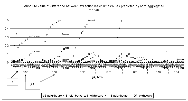
Figure 1. Absolute value of difference between attraction basin limit values predicted by the two aggregated models for part of the tested values. We show here the most significant results

3.4

Figure 1 illustrates this comparison. The comparison indicator is the absolute value of "limit of attraction basin value predicted by the aggregated model with fixed neighbourhood size - limit of attraction basin value predicted by the aggregated mode with variable neighbourhood l". We observe that differences increase in value and frequency when the average number of neighbours decreases. Very few differences can be found with 25 neighbours on average, whereas they are very important for 3 neighbours on average.

3.5

From this comparison obtained from a first experimental plan, we define a second experimental plan to be led on the individual-based model. Selected values of the average neighbourhood size, of gA and β chosen for this second experimental design are listed in table 1. We choose to focus on small average neighbourhood sizes.

3.6

The tested values of parameter "initial proportion of A behaviour" are all integer values located in a range of 5% to 7% around the value corresponding to the attraction basin limit predicted by the aggregated model with variable neighbourhood size. In the case where the aggregated model does not predict the attraction basin limit observed for the individual-based model, we add some values. For instance, if we consider an average size of neighbourhood of 5, gA = 0.59, β = 620, the aggregated model with variable neighbourhood predicts the limit of attraction basin for a proportion of 0.50 A behaviour. Thus, first values of "initial proportion of A behaviour" tested with the individual-based model are {0.45, 0.46, 0.47, 0.48, 0.49, 0.50, 0.51, 0.52, 0.53, 0.54, 0.55, 0.56, 0.57}. Since these values appear to correspond to a final state of "100 % of A behaviour", we continue testing all integer various values of "initial proportion of A behaviour" lower than 0.45 until we reach a final state of "0% of A behaviour": {0.44, 0.43, 0.42, 0.41, 0.40, 0.39, 0.38, 0.37, 0.36, 0.35, 0.34, 0.33, 0.32, 0.31, 0.30, 0.29}. You can read this example on figure 3.

Table 1: Experimental design for gA, β and average neighbourhood size — values of experimental design for initial proportion of A in the population are obtained as explained in the paragraph above
Mean size of neighbourhood	gA (behaviour A payoff)	β (level of randomness in decision function)
3	0,51	7 - 8 - 9 - 10 - 11 - 12 - 13 - 17 - 30 - 25 - 45 - 50 - 60 - 70 - 80 - 90 - 100 - 200 - 300 - 400 - 700
	0,57	12 - 16 - 21 - 23 - 35 - 240 - 940
5	0,55	7,6 - 8 - 10 - 12 - 14 - 16 - 20 - 25 - 50 - 60 - 80 - 250 - 500 - 800 - 1200
	0,59	8,98 - 10 - 11 - 13 - 15 - 20 - 25 - 60 - 250 - 470 - 620 - 800 - 1200
	0,6	9,46 - 9,6 - 10 - 11 - 12 - 13 - 14 - 15 - 17 - 20 - 25 - 26 - 30 - 32 - 38 - 40 - 50 - 60 - 80 - 100 - 120 - 140 - 160 - 200 - 260 - 300 - 800 - 1200
	0,61	12 - 14 - 16 - 18 - 20 - 23 - 27 - 30 - 40 - 50 - 60 - 70 - 80 - 90 - 100 - 150 - 200 - 300 - 400 - 500 - 600 - 700 - 800 - 1200
	0,65	13,1 - 15 - 16 - 25 - 30 - 40 - 60 - 100 - 800 - 1200
	0,67	14,6 - 18 - 19 - 20 - 22 - 25 - 30 - 35 - 80 - 100 - 230 - 320 - 470 - 650 - 800 - 1200
	0,7	18,1 - 22 - 25 - 27 - 28 - 29 - 30 - 35 - 60 - 110 - 250 - 470 - 800 - 1200
8	0,66	11 - 12 - 13 - 14 - 15 - 16 - 18 - 25 - 40 - 130 - 220 - 320 - 620
	0,67	11 - 12 - 13 - 14 - 15 - 16 - 18 - 25 - 40 - 130 - 220 - 320 - 620
	0,74	20 - 21 - 22 - 23 - 24 - 25 - 40 - 130 - 220 - 320 - 620
	0,75	21 - 22 - 23 - 24 - 25 - 27 - 30 - 33 - 36 - 40 - 130 - 220 - 320 - 620
	0,76	21 - 22 - 23 - 24 - 25 - 27 - 30 - 33 - 36 - 40 - 130 - 220 - 320 - 620
25	0,84	31 - 32 - 33 - 35 - 40 - 45 - 50 - 55 - 60 - 65 - 70 - 90 - 110 - 130 - 150 - 170 - 220 - 270 - 320 - 420 - 520 - 620 - 720

3.7

As we explained in a previous article (Edwards et al. 2003a), the equilibrium states of the aggregated models can be found by considering the values of p_A for which dp_A=0. We use the same method here.

3.8

We compare these results with the individual-based model simulations for 200 time steps with 10.000 individuals. One time step corresponds to the asynchronous updating of all individuals of the population. We notice that the speed of quasi-convergence of the individual-based model varies depending on whether the model is tested with values allowing to reach the attractor or the limit of the attraction basin. It goes very quickly to its final state when it corresponds to attractor values (about 5 iterations) and becomes longer when the final state bring closer to the limit of attraction basin. In this case, 200 time steps allow generally to define the final state. For few particular transition states, simulations with more than 200 times steps have been run. 50 runs are performed for each combination of parameter settings.

Simulation Results

3.9

The model with variable neighbourhood size is closer to the individual-based model in most cases than the one with fixed neighbourhood size. However, some differences remain between the individual-based model and the aggregated model with variable neighbourhood size.

A Global Improvement of the Approximation

3.10

In order to have measures to compare the models, we define the following thresholds. They correspond to attraction basin limits for the three models:

• Let IBM₅ be the lowest initial proportion of behaviour A which allows to obtain at least 5% of behaviours A as final state (for the individual based model);
• Let IBM₉₉ be the lowest initial proportion of A behaviours which allows us to obtain at least 99% of behaviour A as final state (for the individual based model) or the lowest initial proportion of behaviour A for which the model converged to a value close to 100% of A (notice that for three neighbours and gA = 0.51 and 0.57, the model never gives 100% of A ; it stops to a value comprised between 90% of A for low value of β and 96% of A for high values of β because of the large proportion of individuals which has 0 neighbours when the average of the connectivity is low (this part has a totally stochastic decision) ;
• A_b the highest initial proportion of behaviour A which allows us to obtain 0% of behaviour A as final state (for both aggregated models).

3.11

Values between IBM₅ and IBM₉₉ correspond to initial proportions of A behaviours for which the individual-based model's final states are unstable: this indicates that the model is changing its attraction basin. We consider models as different when the value of attraction basin limit of the aggregated model (A_b) is outside the range of values corresponding to the change of attraction basin for the individual-based model.

3.12

We measure this difference by a distance D. This distance permits us to evaluate if the aggregated model with variable neighbourhood size has really improved the approximation of the individual based model. This distance between the aggregated model and the individual-based model is:

(17)

3.13

The modality "No error" corresponds to an attraction basin limit of the aggregated model situated in the zone of attractor change for the individual-based model (cf. figure 3 for example).

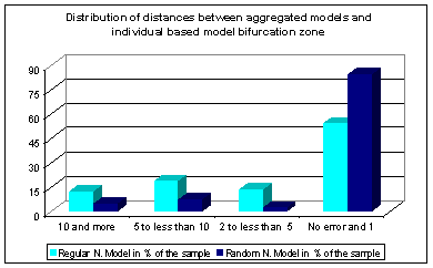
3.14

Results are presented in figure 2 below in which D is grouped following its value into three intervals plus the modality "no error and 1". The value 1 is comprised in "no error" because the derivative result has a precision of ± 1% of necessary initial A to change of equilibrium.

Figure 2. Global improvement of our approximation

3.15

The aggregated model with variable neighbourhood size predicts in most cases the correct value for the attractor change of the individual-based model. It results appear significantly better than the aggregated model assuming a regular neighbourhood. We notice that the aggregated model with variable neighbourhood size approximates well the individual based model in 85% of the cases while the aggregated model with the fixed neighbourhood does so in only 55% of the cases. Moreover, when an error still exists, the variable neighbourhood size model always makes it in less cases than the regular network model.

3.16

After this bird's eye view, let us get a closer view of the results and the error produced by the new aggregated model.

A Better Approximation But Can Be Still Locally Significantly Wrong

3.17

From where does the residual error of approximation come? Let us look at the graphs below, which present some of the results.

3.18

For all these graphs, we distinguish three zones which corresponds to three individual-based model final states:

• The darker zone represents all the initial conditions which lead to 0% of A behaviour for the final state;
• The light orange zone represents all the initial conditions for which the model is changing attractor (i.e. unstable zone);
• The white zone represents all the initial conditions, which lead to 100% of A behaviour for the final state.

A commented illustration is in figure 3.

3.19

We compare the conditions of change of attractor for the three models in the case of a network with 5 neighbours on average (figure 3). We see that in most cases, the aggregated model with variable neighbourhood size succeeds in predicting the attractor's change in the interval where it occurs for the individual based model (with a precision of ± 1% of initial behaviour A). However, for a high value of gA (0.7) and a low value of β (28, 29), both aggregated models predict two attractors although the individual based model has only one. The same is true for gA equal to 0.65 and 0.67. Notice that, similarly, for an average neighbourhood size of 8 and gA equal to 0.74, 0.75 and 0.76, two attractors are predicted by the aggregated models when there exists only one for the individual based model even though no difference is observed for gA=0.66.

Figure 3. Three models bifurcations conditions for 5 neighbours on average

3.20

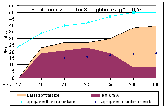
For 3 neighbours on average, we observe another type of error (see figure 4). For gA equal to 0.57 and a low value of β (16), the aggregated model with variable neighbourhood size predicts one attractor while the individual based model has two. Moreover, always for low values of β (21, 23, 35), the approximation of the initial condition needed for attractor's transition is bad. For gA equal to 0.51, no difference is observed.

Figure 4. Three models bifurcations conditions for 3 neighbours mean

3.21

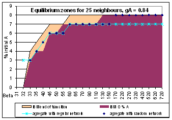
Figure 5 confirms the approximation quality of aggregated models for large average neighbourhood sizes, as well as the better accuracy of the variable neighbourhood approximation.

Figure 5. Three models bifurcations conditions for 25 neighbours mean

3.22

It seems in general that the differences appear for low values of β and high values of gA relatively to the neighbourhood size: the aggregated model with variable neighbourhood size foresees two attractors for gA ≤ 0.59 when the average neighbourhood is 3; for gA ≤ 0.74 when the average neighbourhood is 5; for gA ≤ 0.8 when the average neighbourhood is 8.

3.23

Moreover, we keep in mind that there is no difference for a high value of average neighbourhood size while they exist for small average neighbourhood sizes (3, 5, 8 neighbours). We notice that when the average neighbourhood size is 25, the probability of having exactly 3, 5 or 8 neighbours is too small to be considered significant here.

3.24

The variable neighbourhood aggregated model predicts often the correct value for the attractor change of individual-based, more often than the regular neighbourhood aggregated model.

3.25

However, there remain some final state differences between aggregated and individual-based model when the following three conditions are filled:

• β is weak (lowest values of β which allow the individual-based model to join the stable attractors zone);
• and
• gA takes the highest values in the parameter zone where the model has two stable attractors (for superior gA values, the final state model is always 100% A behaviours);
• and
• The average neighbourhood size is small (less than 10 neighbours).

3.26

We distinguish two types of difference:

1. the variable neighbourhood aggregated model has two final states; it is sensitive to the initial proportion of A while the individual-based model has only one final state (cases 5 and 8 neighbours on average).
2. the variable neighbourhood aggregated model is not sensitive to the initial proportion of A and always has a 100% A behaviours final state while the individual-based model has two final states (case 3 neighbours on average).

A Possible Explanation of the Difference between the IBM and the Variable Neighbourhood Aggregated Model

4.1

In the first case, the remaining difference, between the individual-based and the variable neighbourhood aggregated model, can be explained by the individual-based model's ability to maintain a minority behaviour, which becomes a majority when a set of favourable random events occurs.

4.2

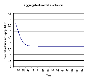
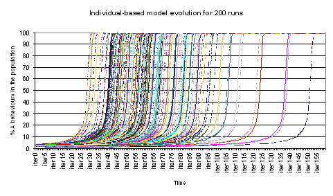
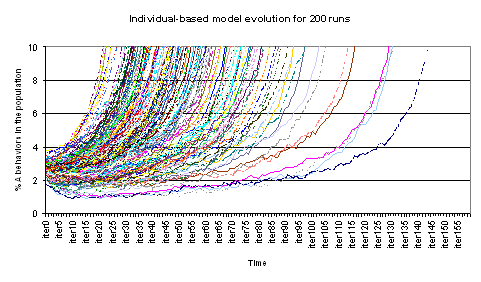
On figures 6 and 7, we observe that the individual-based model always goes to 100% A behaviour even if a long time is necessary (see 7a). It generally begins by decreasing, then stabilises for a variable length of time, then increases slowly and finally dramatically (see 7b). The aggregated model goes to a plateau of 1.73% of A behaviours after a decrease from 4% to 1.73% (see 6).

Figure 6. Evolution of % A behaviours for the variable neighbourhood aggregated model for β = 29, gA=0.7, 5 neighbours and 4% initial A behaviours

Figure 7a. Evolution of % A behaviours for the variable neighbourhood aggregated model for β = 29, gA=0.7, 5 neighbours and 4% initial A behaviours

Figure 7b. Details on the evolution of % A behaviours on time for the individual-based model for 200 runs for β = 29, gA=0.7, 5 neighbours and 4% initial A behaviours

4.3

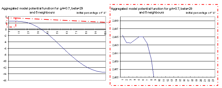
We have noticed that both models can maintain a minority, at least for a certain time for the individual based model. The difference is due to the fact that the aggregated model has no stochasticity to allow the minority to spread. Let's see figure 8 which presents the aggregated model potential function (see equation 16).

Figure 8. Aggregated model potential function for β = 29, gA=0.7, 5 neighbours

The potential function shows that the aggregated model cannot increase to 100 % of A behaviour when it begins with less than 5% of A behaviour (see the zoom on the right hand side), because it is caught in the potential minimum which appears in the zoom. The stochastic events taking place in the individual based model allow it to climb out and to join 100% of A behaviour.

4.4

In the second case of difference, for which the aggregated model goes to 100% of A behaviours while the individual based model converges to a percentage of A behaviours close to 0, the difference is easier to understand. It can be totally explained by the fact that, in the aggregated model, A behaviours obtained by the individual with 0 neighbours (who has in consequence a random decision) influence, at the next step, the individuals of all neighbourhood sizes through the equation 10. The aggregated model makes indeed the assumption that A behaviours are, at each time, homogeneously distributed on the social network. On the contrary, in the individual based model, the A behaviour which has been adopted by individuals with 0 neighbour can not have an effect on the behaviour of individuals with one or more neighbours. The A behaviour is in consequence artificially favoured and can be spread to the entire population whereas it is not the case in the individual based model.

Discussion — Conclusion

5.1

We worked on a simplified version of a classical threshold model. We have just considered the case where all have the same personal interest fixed to zero. To be as general as possible, we place ourselves in the case where little is known about the interactions and therefore consider a random network. A previous work compared this model to an aggregated approximation, based on a simplification assuming a fixed neighbourhood size. In this paper, we propose a refined version of aggregated approximation, based on a Poisson distribution of the neighbourhood sizes.

5.2

The comparison between the three models points out that the variable neighbourhood aggregated model better predicts the final state of the individual based model. This underlines the major role of the network characteristics, and more particularly of the node degree variability in the diffusion dynamics. Indeed the average degree of connectivity (first aggregated model) appears to be not sufficient for characterising the evolution.

5.3

Indeed the aggregated model is in itself a tool to formalise and test possible links between assumptions at the individual level and collective behaviours. Through its simplifying hypotheses, it permits to test the pre-eminence of specific factors on the dynamics. It can also be an approximate substitute to analytical resolution when such a resolution is made impossible by the complexity of the IBM.

5.4

The results of this article show that the node variability has an impact on the diffusion dynamics, particularly on the non-linear phenomena observed in the transition zone between the attractors. Indeed in this zone the network characteristics determine whether the A-behaviour spreads or not in the population. Strong variability of the IBM outcomes can be linked firstly to the persistence or disappearance of the A-behaviour in isolated groups (and so to the connectedness of the interaction network) but also secondly to the variety of dynamics introduced by a heterogeneous interaction network. Indeed even when hypothesizing a homogeneous connectivity degree, the value of this degree can lead to very different dynamics.

5.5

However, there remain some differences between individual based and the refined aggregated model. We showed that this happens in particular when the aggregated model is caught in a very small local minimum of its potential. This minimum is not stable for the individual based model, because the stochastic events are strong enough to extract it from such a minimum, and send it to a much deeper one.

Acknowledgements

This work has been led partly under the responsibility of Laurent Deroussi and Michel Gourgand from LIMOS (University Blaise Pascal of Clermont-Ferrand). I thank them for their support.

References

AXELROD, R. (1995) "Convergence and stability of cultures: local convergence and global polarization". Ann Arbor, Institute of Public Policies Study 34, University of Michigan.

BEN-NAIM, E., Krapivsky, P.L., Vazquez, K.F. and Redner S. (2003) Unity and discord in opinion dynamics. Physica A. 330(1-2): 99-106.

BLUME, L. (1993) The statistical mechanics of strategic interaction. Games and economic behaviour 4:387-424.

BLUME, L. (1995) The statistical mechanics of best-response strategy revision. Games and economic behaviour 11:111-145.

de ANGELIS, D.L., Gross, L.J. Editors (1992) Individual-based models and approaches in ecology, Chapman & Hall .

DUBOZ, R., Ramat, E., Preux, P. (2003) "Scale transfer modelling : using emergent computation for coupling an ordinary differential equation system with a reactive individual model". Systems Analysis Modelling Simulation, 43(6): 793-814.

EDWARDS, M., Huet, S., Goreaud, F., Deffuant, G. (2003a) Comparing individual-based model of behaviour diffusion with its mean field aggregated approximation. Journal of Artificial Societies and Social Simulation 6(4) https://www.jasss.org/6/4/9.html.

EDWARDS, M., Huet, S., Goreaud, F., Deffuant, G. (2003b) Comparaison entre un modèle individu-centré de diffusion de l'innovation et sa version agrégée dérivée par champ moyen pour des simulations à court terme. Actes du colloque Modèles Formels d'Interactions91-100, éditeurs: A. Herzig, B. Chaib-draa. Ph. Mathieu Cépaduès-éditions.

ELLISON, G. (1993) Learning, Social interaction, and coordination. Econometrica 61:1047-71.

EPSTEIN, J. and Axtell, R. (1996) Growing artificial societies: Social science from the bottom up. Cambridge Massachussetts, MIT Press.

FAHSE, L., Wissel, C., Grimm, V. (1998) Reconciling classical and individual-based approaches of theoretical population ecology: a protocol to extract population parameters from individual-based models. American Naturalist 152:838-852.

GILBERT, N., Troitzsch, K. G. (1999) Simulation for the social scientist Open University Press.

GRANOVETTER, M. (1978) Threshold models of collective behaviour. American Journal of Sociology 83:1360-1380.

GRIMM, V. (1999) Ten years of individual-based modelling in ecology: what we have learned and what could we learn in the future?, Ecological Modelling, 115:129-148.

KIRKPATRICK, S., Gelatt, C.D., Vecchi, M.P. (1983) Optimization by Simulated Annealing, Science, 220(4598):671-680.

LUCE, R.D. (1959) Individual Choice Behaviour: a Theoretical Analysis, 1979, Greenwood Press Reprint.

MORRIS, S. (1997) "Contagion". Working paper, Department of Economics, University of Pennsylvania.

PICARD, N. and Franc, A. (2001) Aggregation of an individual-based space-dependant model of forest dynamics into distribution-based and space-independant models, Ecological Modelling 145:68-84.

VALENTE, T.W. (1995) Network models of the diffusion of innovations. Cresskill, New Jersey: Hampton Press, Inc.

WEIDLICH, W. (2000) SocioDynamics: a Systematic Approach to Mathematical Modelling. Harwood.

WEIDLICH, W. (2002) Sociodynamics: a systematic approach to mathematical modelling in the social sciences. Nonlinear Phenomena in Complex Systems, 5(4): 479-487.

YOUNG, P. (1998) Individual Strategy and Social Structure, Princeton University Press.

YOUNG, P. (1999) Diffusion in Social Networks, Working Paper No 2., Brookings Institution.

Return to Contents of this issue

© Copyright Journal of Artificial Societies and Social Simulation, [2007]