Journal of Artificial Societies and Social Simulation vol. 1, no. 3, <https://www.jasss.org/1/3/1.html>

Abstract

The article argues that using cellular automata (CA) is a promising modelling approach to understand social dynamics. The first section introduces and illustrates the concept of CA. Section 2 gives a short history of CA in the social sciences. Section 3 describes and analyses a more complicated model of evolving support networks. The final section summarises the advantages of the CA approach.

Keywords:

cellular automata, social dynamics, modelling

Introduction

1.1

In 1884, Edwin A. Abbott published a work of mathematical science fiction entitled Flatland - A Romance of Many Dimensions under the pseudonym "A. Square" (Abbott 1987). Square is presented as an inhabitant of Flatland which, as its name suggests, is a two-dimensional world. What is more, A. Square is a square. The decisive event in the novel is a strange encounter between Square and Sphere, a solid and three-dimensional being. For some hours, Sphere gives Square an opportunity to look at Flatland from "above", a previously unimaginable perspective. Square learns that there is a third dimension with extraordinary properties. By entering it, one can leave rooms which Flatlanders regard as closed and enter them again wherever one wants. However, in Flatland, expressing the view that a third dimension exists is forbidden by law. Square tries hard but cannot avoid talking about what he has experienced. From time to time he expresses solidarity with the lunatic underground whose members believe in a third dimension populated by spheres and cubes. On one occasion, he observes that prophets and inspired people are always considered mad by the majority. On another, he describes his voyage in space - although he presents it as an imaginary event in the first instance. Not surprisingly, Square is arrested. Although the court is sympathetic to his defence, he fails to convince them on two counts. Firstly, he is not able to explain his notion of "upwards" and the way in which it differs from "northwards". Secondly, he cannot provide a convincing description of what he is pleased to call a "cube". As a result, Square is sentenced to comfortable but permanent imprisonment. At the end of the novel, after he has already served seven years in prison, Square states: "It is part of the martyrdom which I endure for the cause of the Truth that there are seasons of mental weakness, when Cubes and Spheres flit away into the background of scarce-possible existences; when the Land of Three Dimensions seems almost as visionary as the Land of One or None; nay, when even this hard wall that bars me from my freedom, these very tablets on which I am writing, and all the substantial realities of Flatland itself, appear not better than the offspring of a diseased imagination, or the baseless fabric of a dream" (Abbott 1987, p. 91).

Cellular Automata and the Idea of Low Dimensional Societies

2.1

Square's memoirs are a plea to think about higher dimensions and the book is devoted to readers willing to do so. However, despite the sympathy that brave Square deserves, this paper takes the opposite approach: we seek to demonstrate that models based on rigorous simplification (especially those that one might call Flatland or checkerboard models) are a promising method for understanding our real world of higher dimensions.

2.2

The class of models I will focus on are called cellular automata (CA). The basic features of a CA are:^[1]

• Cells are arranged in a regular D-dimensional grid.
• Every cell adopts a state from a finite set of states.
• Time is discrete.
• Cells change their states according to local rules.
• The same transition rule applies to all cells.
• In each period cells are updated (simultaneously or sequentially).

2.3

In this paper, we will show that low-dimensional (and especially two-dimensional) CA are a promising modelling approach for understanding social dynamics. In the remainder of this section, the basics of CA modelling are introduced and illustrated. Section 2 provides a short history of CA in the social sciences and illustrates typical insights produced by CA based models. Section 3 describes and analyses a more complicated CA model of evolving support networks. This section also explores the claim that effective use of CA is more likely to be endangered by excessive complexity than by simplicity. Section 4 concludes and summarises the advantages of a CA approach.

2.4

A basic feature of CA is the assumption of discrete space or an underlying grid structure. Figure 1 provides examples of possible lattices for a two-dimensional CA. To the left we have a finite 9×9 grid. To the right, the corresponding edges of another finite grid have been "pasted together", resulting in a three-dimensional solid called a torus.

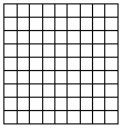
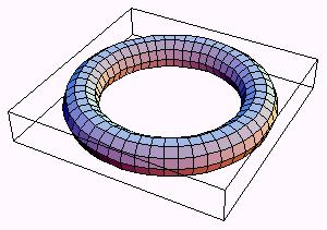
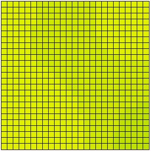
Figure 1: Two-dimensional CA. Left: without edges pasted. Right: with edges pasted.

2.5

A second decisive feature of a CA is locality. This means that all interactions take place only within well defined spatial neighbourhoods. Figure 2 illustrates three different kinds of neighbourhoods in a two-dimensional lattice. Figure 2a shows the so-called von Neumann neighbourhood. For this type of neighbourhood, cells to the north, south, east and west of the dark centre cell are defined as neighbours. Since the centre cell is always part of its own neighbourhood by definition, the centre cell has 5 neighbours in total. In Figure 2b and 2c, Moore neighbourhoods of different sizes are shown. A Moore neighbourhood also includes diagonal cells to the north east, north west, south east and south west. These always form a square pattern. Obviously Moore neighbourhoods of all sizes are possible, subject only to the dimensions of a given cellular world.

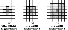
Figure 2: Different neighbourhood templates.

2.6

Von Neumann and Moore neighbourhoods are based on a rectangular grid structure. However, triangular, hexagonal and irregular grid structures are also possible (Hegselmann et al. 1998).

2.7

To illustrate the other essential features of the CA approach, we will present a simple model of opinion dynamics.^[2] We assume a finite, rectangular, 2-dimensional grid and von Neumann neighbourhoods. All cells are occupied by individuals i who have opinions. These opinions are the states of our cells. They are taken from the real interval [0, 1]. Individuals update their opinions by averaging over the opinions of all their neighbours. (Recall that each individual is part of their own neighbourhood.) The same weight is given to the opinion of each neighbour. Let u_j(t) stand for an individual j's opinion in period t, N_i for the set of i's neighbours and #N_i for the number of neighbours. This gives:

.

[1]

2.8

A problem arises because without any "correction", this type of averaging leads to an infinite set of possible opinions. By definition, the number of states should be finite in a classical CA. We therefore transform [1] to satisfy the requirement of a finite opinion space. A finite number of opinions is produced by discretising the infinite set of opinion values using the functions shown in Figure 3.

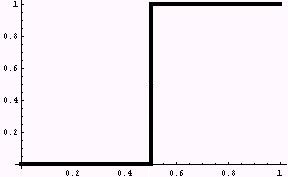
if x < 1/2, then y = 0 if x >= 1/2, then y = 1

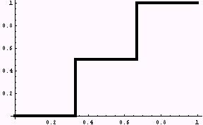
if x < 1/3, then y = 0 if x >= 1/3 and x < 2/3, then y = 0.5 if x >= 2/3, then y = 1

Figure 3. Top: two possible opinions (0 and 1). Bottom: three possible opinions (0, 0.5, and 1).

2.9

The possible values of the step functions are the only opinions which can be held. Those values are the input to which we apply the dynamics given by [1]. The result is an opinion u_i^*(t+1) that in most cases is not in the set of possible opinions. However, the step function then returns u_i^*(t+1) for an opinion u_i(t+1) and that is invariably one of the finite set of possible opinions. Subsequently, this output opinion is used as the input for the next period and so on.^[3] In short, the procedure to keep opinions discrete is:^[4]

.

[2]

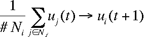
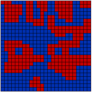
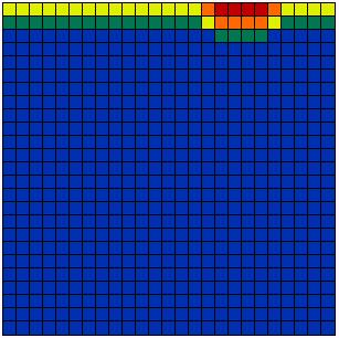
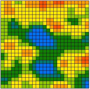
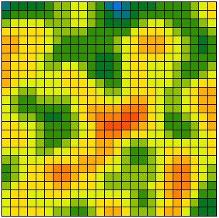
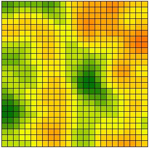
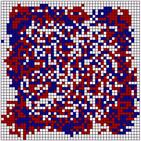
[2] is the universal transition rule. It is applied sequentially to randomly selected cells, which is to say that the updating procedure used is sequential updating. (Simultaneous updating involves simultaneously applying [2] to all cells.) Figure 4 shows the typical results of simulation runs with 2, 5, 10, 15, and 30 different opinions. At the beginning all possible opinions have the same frequency in the population. Obviously in all cases, opinion patterns and clusters emerge. The structures shown are stable for ever. In the continuous case shown in Figure 4(f), no step function is applied and the dynamics are driven by [1] instead of [2]. It can be proved analytically that these dynamics always lead to ubiquitous agreement when t tends to infinity (Hegselmann et al. 1998).

(a) 2 possible opinions	(b) 5 possible opinions
(c) 10 possible opinions	(d) 15 possible opinions
(e) 30 possible opinions	(f) continuous opinions
color coding of opinions
Figure 4: Results of simulation runs with 2, 5, 10, 15 or 30 discrete opinions and with continuous opinions.

2.10

Figure 4 suggests that the more possible opinions there are, the closer the stable results get to universal consensus and the smoother are the transitions between areas of differing opinion. This observation is borne out by the results of further simulation runs shown in Figure 5. The x-axis indicates the number of different opinions for differing degrees of discretisation. The first degree of discretisation yields just 2 opinions, 0 and 1. The second produces 3 opinions: 0, 0.5 and 1. The final degree produces 50 possible opinions. For each degree of discretisation, picture the y-axis divided into intervals corresponding to the appropriate step function so that the y-axis, ranging from 0 to 1, is divided into 2 intervals for 2 opinions, into 3 for 3 opinions and so forth - although this is not directly visible in Figure 5. We then colour each interval to show the frequency of individuals with that opinion after the system has stabilised. For reliability, we computed the mean frequency of 10 simulation runs per degree of discretisation. The simulations were run on a finite 25 × 25 grid with sequential updating, von Neumann neighbourhoods, step functions like those in Figure 2 and dynamics given by [2].

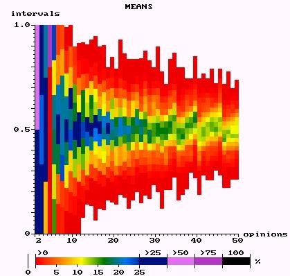
Figure 5: Discrete opinion dynamics with up to 50 possible opinions: Mean frequencies of opinions after convergence.

2.11

Figure 5 demonstrates that discretisation of opinions matters a lot. While a system with continuous opinions ends up in ubiquitous agreement, we obtain stable polarisation for discrete opinion change, a dramatically different result. Moreover, Figure 5 shows that the closer we get to the continuous opinion case, the more the stable end configuration is centred on the middle of the opinion space.

2.12

The model just described illustrates some important points about CA based modelling of social dynamics:

• CA models cover basic features of a significant class of social processes in the real world: Over a period of time numerous people interact, interactions and information are local and the neighbourhoods of interaction overlap. Therefore, the CA framework provides a multi agent system that is based on locality and overlapping interaction structures.
• CA based models make it quite clear how certain macro effects are dynamic consequences of decisions and mechanisms operating only at the micro level. Order, structure, clustering and segregation are all generated by such micro level rules. The basic features of CA make it almost impossible not to focus on the evolution of macro structure and emergence of macro properties. From this perspective, we can expect that CA based modelling will contribute to a better understanding of micro/macro relations.^[5]
• An essential feature of CA is discretisation of space, time and state. The model above illustrates that discretisation can matter. The qualitative behaviour of discrete dynamics may be quite different from that in the continuous case. Therefore, if carried out incautiously, CA based modelling may produce artefacts!^[6]

In short, though its use is not always completely transparent, CA based modelling seems to be a promising approach for providing a better understanding of social processes.

A Short History of CA Based Modelling in the Social Sciences

3.1

In the natural sciences CA were introduced by John von Neumann and Stanislaw Ulam at the end of the nineteen forties (Neumann 1966) mainly to provide a reductionist abstractions of life and self-reproducing systems. Usually CA based models require a lot of iterated computations. Since computers have become more widely available, many new CA based models have been developed in science and engineering. Nowadays they are used extensively in applications ranging from crystal growth, soil erosion, diffusion and fluid dynamics to modelling the collisions of galaxies (Burks 1970, Demongeot et al. 1985, Wolfram 1986, Toffoli and Margolus 1987, Gutowitz 1991). Moreover, CA can be regarded as parallel processing computers and are therefore of interest to computer scientists. Preliminary steps towards a classification of CA have been made (Wolfram 1984) but analytical understanding has generally remained poor. For this reason, simulation has continued to play an important role in CA research.

3.2

It appears that CA based modelling started at about the same time in the social and natural sciences. James M. Sakoda was the first person to develop a CA based model in the social sciences. The model did not see the light of the day as part of the CA literature at the time or make any reference to previous CA research. It was baptised a "checkerboard model". Sakoda published the article The Checkerboard Model of Social Interaction in 1971^[7] but the basic design of the model was already present in his unpublished dissertation of 1949. The central goal of his model was to understand group formation. The model "grew out of an attempt to portray the interaction in a relocation center during World War II" (Sakoda 1971, p. 120), where members of the Japanese minority in the US were evacuated after Japan's attack on Pearl Harbour.

3.3

In Sakoda's model, members of two groups are living on a checkerboard. They have positive, neutral or negative attitudes to each other, called valences. These valences are given by integers. V_ij is the valence of an individual j for an individual i. P is the set of all individuals and not all cells are occupied. Individuals get the chance to move to empty sites in their 3 × 3 neighbourhood. If there are no empty cells then an individual is permitted to jump over one cell but migration is always local or permitted only within certain limits. An individual i uses a migration option to move to sites where:

.

[4]

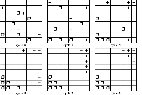
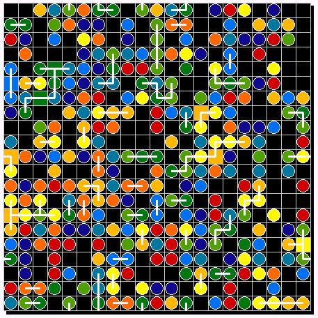
is maximised. d is the Euclidean distance between i and j. w determines how strongly valences are discounted by distance. The greater w, the less the valences are discounted by distance. Sakoda's world is an 8 × 8 checkerboard occupied by two groups, each with 6 members. The members of one group are represented as squares and members of the other as crosses. Sakoda analyses different combinations of attitudes. One of these is called segregation, another is called suspicion. These attitudes are shown in Figure 6.

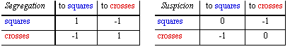
Figure 6: The attitude combinations segregation and suspicion.

3.4

Figure 7 shows the dynamics of group formation under the attitude combination called segregation. It takes very little time before the two groups have organised themselves.

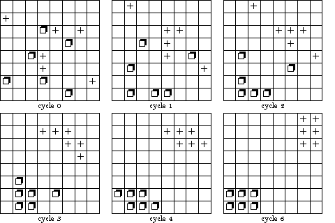
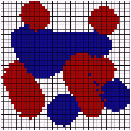
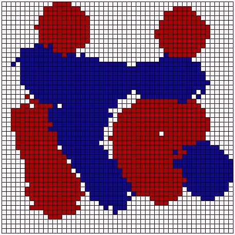
Figure 7: The dynamics of segregation (Sakoda 1971, p. 127).

3.5

It is no surprise that the segregation attitude combination leads to two groups living in opposite corners as shown in Figure 7. But the dynamics of suspicion shown in Figure 8 are a surprise:

Figure 8: The dynamics of suspicion (Sakoda 1971, p. 126).

3.6

Obviously individuals with neutral attitudes to each other may nevertheless form a segregated group, driven only by negative attitudes to members of another group. However, there is something even more surprising which was not observed by Sakoda: a negative attitude towards the other group combined with indifference towards one's own group may lead to much more massive clusters than under positive feelings for one's own group. To see this effect, larger groups living on larger checkerboards are necessary, something that nowadays can easily be done even with the cheapest computers. Figure 9 demonstrates the effect in a 40 × 40 world which has groups with 180 members each. "Squares" are now blue cells and "crosses" are red ones. Everything else is kept constant in the replication.

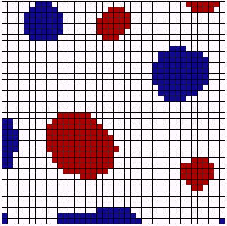
Figure 9. Left: segregation Right: suspicion. Both dynamics were started with the same random distribution of cells.

3.7

Once this effect has been observed, it is not difficult to explain why neutral attitudes towards one's own group leads to more complete polarisation and clustering. Both attitude patterns, segregation and suspicion, motivate people to run away from members of the other group. If, under the segregation attitude pattern, members of the same group meet each other while fleeing, the meeting point acquires attraction and may become attractive enough to cause those meeting to stay where they are. Under indifference towards one's own group, this is not the case and getting as far away from the others group as possible is the only objective. As an unintended consequence people end up living in one massive cluster of their own colour - with the exception of one blue and one red person who did not escape fast enough and became immured.

3.8

These results underline that CA based modelling may contribute to "insight into basic principles of behavior" (Sakoda 1971, p. 121) and especially to a better understanding of micro/macro relations in dynamic social processes. At the same time there is a methodological lesson which is that, for certain effects, the size of a cellular world may matter!

3.9

Another early - and much better known - example of CA based modelling was provided by Thomas Schelling.^[8] In Schelling (1969) he analyses segregation processes. Individuals are assumed to live on a line and belong to two different classes: black and white or, in more abstract terms, stars and zeros. Each individual is in a Moore neighbourhood and receives migration options. Individuals use these to leave their actual neighbourhood if it does not have a required minimum frequency of individuals of their own class. For instance, individuals might wish to live in a neighbourhood where their class is not in a minority. If that requirement is not met, an individual will move to the nearest alternative site where it is. Schelling (1971) elaborates the model and analyses it in more in detail, in particular using a two-dimensional checkerboard world to represent the underlying spatial structure.

3.10

Figure 10 demonstrates the results of a neighbourhood formation process. Individuals tried to find neighbourhoods where they were not in a minority position. Each individual is in a 3 × 3 Moore neighbourhood. It is noteworthy that Schelling did the simulations without using a computer.

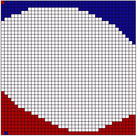
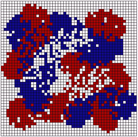
Figure 10. Left: random distribution (Schelling 1971, p. 155). Right: segregation (Schelling 1971, p. 157).

3.11

Obviously an extremely high degree of segregation may result from decisions based only on the principle that an individual does not want to live in a minority. Even with a neighbourhood preference which requires as little as 30% of one's own group, we still obtain severe segregation as Figure 11 demonstrates, based on a replication of Schelling's model by computer simulations. All four simulations start with the same random distribution of blue and red cells. The neighbourhood size is 11 × 11 and empty cells count as "others". Dissatisfied individuals move to locations which are as near as possible to their neighbourhood preference. They are indifferent between all locations which meet their neighbourhood preference.

Preference: <= 90%	Preference: <= 50%
Preference: <= 30%	Preference: <= 20%
Figure 11: Experiments with different neighborhood preferences.

3.12

Obviously, a high degree of segregation occurs whether individuals only dislike being in a minority position or are far more clannish and require at least 90% of their own kind in the neighbourhood. Only a neighbourhood preference of significantly less than 30% for one's own group can prevent severe segregation. As in Sakoda's case, the fundamental insight is again that rules applied on a micro level may produce macro effects that are surprising from the researcher's perspective and unintended from the actor's point of view.

3.13

Sakoda never referred to CA and neither did Schelling. The concept (as used in the natural sciences) was obviously not known to them at the beginning of the seventies. Nevertheless, checkerboard models share with CA basic features like discrete space, discrete time and the importance of neighbourhoods and locality. That the checkerboard models of both Schelling and Sakoda essentially focus on migration (moving around and looking for partners or attractive neighbourhoods) does not matter: moving is just an application of a rule by which an occupied cell and an empty one exchange their states.

3.14

The first person who explicitly classified checkerboard models as CA was the economist Peter S. Albin in his book The Analysis of Complex Socioeconomic Systems (Albin 1975, see also Albin 1998). He was also the first to stress the enormous potential of CA and finite automata for understanding social dynamics.

Nevertheless, it is only within the last decade that CA based models have been used more frequently in the behavioural and social sciences.^[9] In social psychology, Nowak et al. (1990) have developed a two-dimensional CA model of evolution in attitudes. In economics, Keenan and O'Brien (1993) use a one-dimensional CA to model and analyse pricing in a spatial setting. Axelrod (1984, pp. 158ff.) made the first steps in analysing the dynamics of cooperation within a CA framework, although he did not refer to his model as a CA. Nowak and May (1992, 1993) developed the idea and studied the dynamics of cooperation using a two-dimensional CA with two-person games as building blocks. Bruch (1993) and Kirchkamp (1994) follow the same line, but use different and more sophisticated learning rules. The same framework is used in Messick and Liebrand (1995), who analyse the dynamics of three different decision principles.^[10] A substantial number of the artificial societies described in Epstein and Axtell (1996) are based on CA modes. Gaylord and D'Andra (1998) describe a toolkit for CA based modelling of social dynamics using MATHEMATICA.

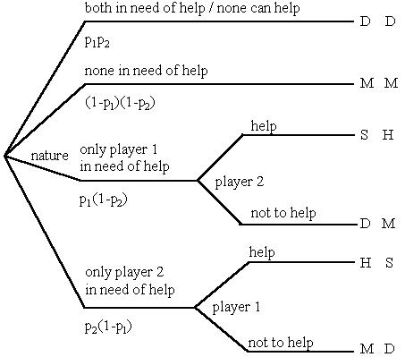
The Evolution of Support Networks^[11]

4.1

The agents and environments in the models described by Sakoda and Schelling are fairly simple. In this section, we present a model in which the agents are more individualistic, have much better developed cognitive capacities and cope with tasks of greater complexity. The central question the model addresses is how networks of mutual support can evolve in a world:

• which is exclusively inhabited by rational egoists,
• who are unequal in that they need help with different probabilities,
• must choose their partners themselves,
• and will choose those partners in opportunistic ways?

4.2

The general idea is to model support relationships using a two person support game. Agents play that game simultaneously with all their neighbours. From time to time, agents get the chance to migrate in their two-dimensional checkerboard world. Migration allows agents to move to neighbourhoods they find more attractive. The following subsections describe the central components of the model in more detail.

(A) Support Game

4.3

The basic game is specified in figure 12. It is a fundamental characteristic of the game that both players will become dependent on help with a certain probability, p₁ or p₂. These probabilities remain constant throughout the game. (1-p₁) and (1-p₂) are therefore the probabilities that player 1 and player 2 will not become needy. The first move of the game is made by Nature. According to the probabilities p₁ and p₂, Nature decides whether both players, only one player, or neither is in need of help. If a player needs help, they cannot help anyone else. On the other hand, a player who is not in need of help has to decide whether they want to help or not. This decision is a move in the game and players who are not able to help cannot make a move. Thus, depending on Nature's chance moves, player 1, player 2 or neither is in a position to make a move.

S :	Saved	D: Drowned	S > D
M:	Move on	H: Help	M > H
p1 :	probability that player 1 will become needy
p2:	probability that player 2 will become needy
0 < p1, p2 < 1
Figure 12: Support game[12]

4.4

Because M > H, neither player will give support to the other at their respective decision nodes. For this reason, not helping at all is a dominant strategy. This remains true even when the mutual support is profitable for both players. That is the case if for both players it holds that:

.

[5]

Provided that the condition in [5] is fulfilled the expected payoff for mutual support is greater than the expected payoff for not giving support to each other. Therefore [5] describes a condition under which the solution of the support game becomes inefficient. If characterised as a matrix game one can easily verify that [5] describes a condition under which the support game turns into a 2-person Prisoner's Dilemma. We will refer to [5] as the PD-condition.

4.5

It is a well-known fact (Taylor 1987, Axelrod 1984, Friedman 1986) that iterated Prisoner's Dilemma games can have cooperative equilibria resulting from "supergame strategies" supporting cooperation in all constituent games. In this sense Prisoner's Dilemma games are "cooperatively soluble", a result which is also applicable to support games.^[13] This result can be interpreted as asserting that cooperative supergame equilibria exist if the probability of being involved in a further iteration of the game is sufficiently high.

An iterated support game has a cooperative solution if and only if, for both players, it holds that:

.

[6]

[6] is based on the assumption that it is only in cases of unilateral emergency that one player can infer whether the other is cooperating or defecting. I will refer to [6] as the COOP-condition.^[14]

(B) Interaction Structure

4.6

It is assumed that individuals belong to nine different risk classes which become needy with probabilities 0.1, 0.2, ... , 0.9. They live on the surface of a torus and the interaction neighbourhood is von Neumann. An initial distribution of individuals and empty cells is randomly generated.

(C) Migration Options

4.7

In each period a random number generator allocates migration options according to an exogenous probability. Individuals are not obliged to use the migration options which are allocated to them. Migration is possible within a certain migration window, but only to vacant destination cells. Migration options are evaluated and used in sequential order according to the results of a lottery. After all migration options have been dealt with, a new period starts. The migration window (a square with a side length which is always an odd number of cells centred on the individual with the migration option) has the same size for all individuals. 11 cells on a side is a typical value.

(D) Generally Accessible Information and Intelligence

4.8

Each individual knows the risk classes of all his real (or potential) neighbours and the payoffs of the support game. The probability of getting migration options is common knowledge and is used to calculate a pessimistic proxy for retaining ones neighbours and therefore having a further round of play with them in the next period. "Pessimistic" means that individuals assume that every migration option will be used. If q is the probability for getting a migration option the probability of stability, a, is (1-q)². Using all this information, each individual decides whether conditions [5] and [6] are fulfilled. If both conditions are met, two neighbours will support each other.^[15] Otherwise, both of them will defect.

(E) Partners Of Different Attractiveness

4.9

Everyone knows that partners of different risk classes are of different attractiveness. All individuals can work out that, relative to their own risk class, they are in the best possible social position when surrounded by four individuals which are members of the best risk class willing to engage in support relationships with them. On the other hand, the worst social positions involve being surrounded by empty cells or individuals with whom support relations are not possible. An individual will be satisfied with any social position which offers a certain fraction of the difference between the payoff in the best and the worst social positions. This fraction is called minimum level. Satisfied individuals will migrate only if they can move to a position which is at least as good as that they currently occupy. Dissatisfied individuals will take every migration option they are offered, even moving to worse locations in the hope of gaining access to better positions which may be accessible from the new location.

4.10

In the following subsections, I will describe three experiments. The initial conditions can be seen in Figure 13. They differ with respect to the probabilities with which individuals get migration options. Note that the possibility of functioning support relations between members of different risk classes is affected by that probability. All other parameters are kept constant.

---

Support Networks

Basics

interaction window:	von Neumann neighbourhood.
migration window:	11 × 11 with the given position in the centre.
world:	21 × 21 (torus).

Class structure
individuals per risk class: 35, giving a total of 315 individuals and 136 empty sites.

Payoffs and minimum level
Saved = 5, Drowned = 1, Move on = 7 and Help = 6 so (S - D) / (M -H) = 4 and the minimum level is 50%.

Probabilities for getting migration options

0.05	=>	a = 0.903 (first experiment)
0.10	=>	a = 0.810 (second experiment)
0.15	=>	a = 0.723 (third experiment)

Use of migration options

• Dissatisfied individuals choose the best alternative location.
• Satisfied individuals move only if the alternative location is at least as good as their current one.
• Individuals who know they cannot find partners at all move randomly.

---

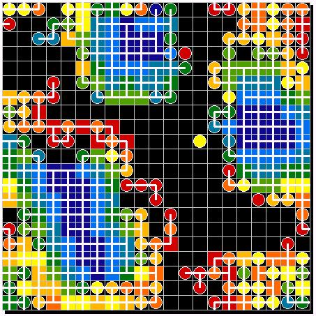
Figure 13: Initial conditions

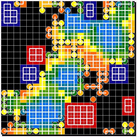
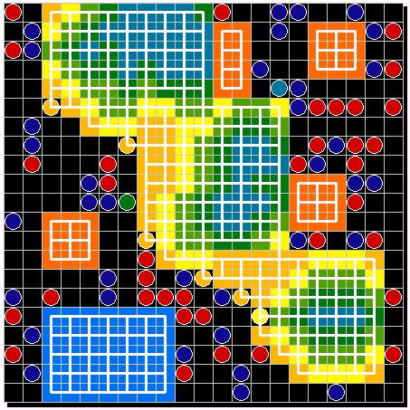
4.11

Figures 14 to 16 show the evolved structures of the different societies after 2000 periods. Each society started with the primordial soup shown in Figure 13. Note that:

• Black cells are empty.
• Round cells are dissatisfied because they either get less than the minimum expected payoff level of 50% or because under the given conditions they do not have any chance of finding partners for mutual support.
• Filled cells are satisfied.
• Short white lines connecting two individuals indicate functioning support relations between them.
• Different colours represent different risk classes according to the legend underneath the figures. Risk class 1 (dark blue) becomes needy with a probability of 0.1, risk class 2 (light blue) with a probability of 0.2 and so on.

Figure 13: primordial soup	Figure 14. First experiment: chance for migration 5%
Figure 15. Second experiment: chance for migration 10%	Figure 16. Third experiment: chance for migration 15%

4.12

Even a superficial inspection makes it clear that well-ordered support networks emerge from the primordial soup. This shows that support networks can evolve even in a world of rational egoists, differently endowed by nature and choosing their partners opportunistically. Closer inspection reveals more interesting details of the support networks.

4.13

In the first experiment, members of class 1 establish support relations mostly amongst themselves. However, some support relations also exist with members of class 2. Members of the latter class live on the perimeter of the areas occupied by class 1. Quite often we find members of class 3 themselves on the perimeter of the areas occupied by class 2, and members of classes 4 and 5 follow the same annular pattern. Class 9 members can find partners only in classes 8 and 9 so members of these classes live as "outcasts" at the outer borders of the network. It is also clear that class segregation is less strong among those in intermediate risk classes.

4.14

In the second experiment, members of the extreme risk classes establish support relations only amongst themselves. In different areas we find closed networks of members of those classes. Members of class 2 seem to form the cores of networks which are often surrounded by members of class 3. Around these, we find members of classes 4 and 5. It is now members of classes 6 and 7 who are living on the edges of the networks. As before, it is individuals in the intermediate risk classes which display the least class segregation.

4.15

In the third experiment, members of classes 1 and 9 cannot find partners at all and it is now classes 2 and 8 whose members establish support networks only amongst themselves. Often members of class 3 form the nucleus for networks in which they are surrounded by members of class 4 with members of classes 5, then 6, around them. The members of class 7 are strongly segregated, living almost entirely as neighbours of either class 6 members or members of their own class.

4.16

For a deeper understanding of this network structure, one should ask two questions:

• Which classes are capable of establishing support relations?
• How attractive are partners from different classes?

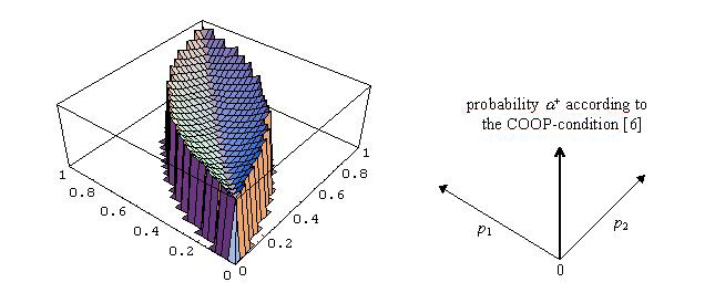
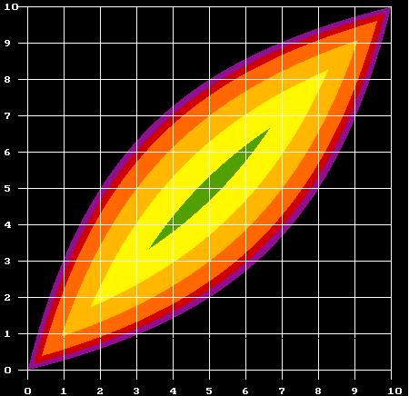
Figure 17: PD and COOP-condition for (S-D)/(M-H) = 4.

4.17

The first question is answered in Figure 17, which presents the PD and COOP-conditions visually. The horizontal axis represents the probabilities of becoming needy (p₁ and p₂). The vertical axis indicates the threshold probability of stability (a⁺) which makes support relations an equilibrium according to [6]. If there is no a⁺ value, then condition [5] is not met and this is a case in which mutual support does not pay off at least for one of the players. Figure 18 is a 2-dimensional version of Figure 17. In Figure 18 the a⁺ value is presented using a colour code.

4.18

Looking at Figures 17 and 18 suggests two conditions for the existence of functioning support relations between different classes:

• The risk classes must not be too far apart.
• Intermediate risk classes may be further apart than extreme risk classes.

4.19

The two figures also suggest two conditions regarding the probability of stability, which is necessary for mutual support:

• The further apart risk classes are, the more stringent the conditions for stability.
• The stringency of the stability conditions rises as the risk classes that are paired become more different in their neediness.

The last point - a direct consequence of [6] - may seem surprising at first glance. The explanation is that two individuals of extreme risk classes are facing a problem which members of intermediate classes only experience to a much lesser degree. It is very likely that two members of the least needy risk class will not need help. Two members of the most needy risk class will probably be in need of help simultaneously and thus neither of them will be in a position to help the other. In both cases, unilateral emergencies become rare events. For this reason, the expected utility of mutual support decreases at the extremes. At the same time, it becomes more difficult to find out whether other individuals are cooperating or defecting. Therefore, probabilities of stability which makes support relations effective for intermediate risk classes may not be sufficient for the extreme risk classes.

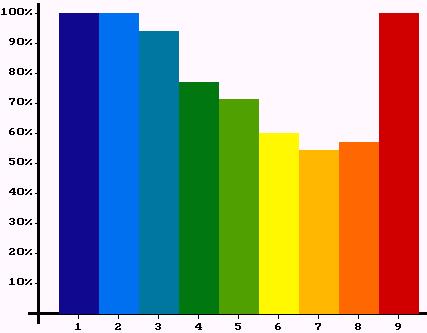
Figure 18: The colours indicate the probability (a+) that has to be exceeded to meet the COOP-condition [6] for a given pairing of risk classes. Black indicates that the PD-condition [5] is not met for that pair of risk classes. As before (S-D)/(M-H) = 4.

4.20

Using these figures, it is easy to explain some of the features of the evolved networks displayed in the experiments. With an increasing probability of getting migration options, the pessimistic proxy for the probability of stability decreases. Therefore the lens shaped area of pairs for which mutual support is a feasible solution shrinks. In the first experiment we have functioning support relations even amongst members of classes 1 and 2 and, furthermore, amongst members of classes 8 and 9. In the second experiment, based on a lower probability of stability, those classes were too far apart to make mutual support a possibility. In the third experiment, mutual support in classes 8 and 9 is also ceases, owing to the fact that the continuing decrease in stability progressively removes the possibility of mutual support for the extreme classes. Figure 19 gives a general overview of problems of pairing in our setting.

RISK CLASS	quite bad	middle risk	quite good
quite bad	COOP-condition tends not to be fulfilled.		COOP and PD-condition tend not to be fulfilled.
middle risk		COOP and PD-condition can comparatively easy be fulfilled.
quite good	COOP and PD-condition tends not to be fulfilled.		COOP-condition tends not to be fulfilled.
Figure 19: Problems of pairing.

4.21

To understand the annular structure of the evolved networks, one cannot only concentrate on pairings for which mutual support is possible. It is also necessary to consider the differential attractiveness of classes. By doing this one finds the answer to the second question posed above. The decisive point is the size of the support surplus (P_ij) which is the difference between the expected benefits and costs for a member of class i engaging in mutual support with a member of class j.

.

[7]

4.22

Only if the surplus is positive will a rational egoist consider engaging in mutual support (the PD-condition). Only if the probability of stability is high enough, will they actually support each other (the COOP-condition). P_ij depends on p_j (the other's probability of becoming needy) and can be maximised by finding a partner belonging to the lowest risk class in which conditions [5] and [6] are still met. Consequently, members of more needy classes try to become neighbours with members of less needy classes with whom support relations are nonetheless feasible. Unfortunately for them, these less needy individual are themselves looking for neighbours who are less needy still. More needy classes are satisfied with less needy neighbours, but it is just that which makes those less needy individuals willing to move. This effect becomes more severe when there are wider possibilities for functioning support relations between different risk classes. The widest possibilities exist in the first experiment, and that is precisely the experiment in which we find the highest frequency of dissatisfied agents (coloured circles). Figure 20 compares the first and second experiments.

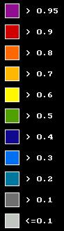
Figure 20: Percentages of satisfied agents in different classes. Left: first experiment. Right: second experiment.

4.23

Since the evolved network structures in both experiments are not totally stable, the frequencies of satisfied individuals fluctuates, but only slightly. Turning to the third experiment, note that the dark blue circles (class 1) and the dark red circles (class 9) are circles only because, with the prevailing probability of stability, there isn't any class with whom they can establish support relations, not even their own. Therefore, under our previous definition of satisfaction, they are satisfied: trivially, they get at least 50% of what they could get if all their neighbours were members of the best risk class willing to engage in mutual support with them because that class is null. Agents are realistic and their view of an ideal neighbourhood is not based on wishful thinking about who is prepared to take part in mutual support relations with them. That explains why, in the first experiment, less than 30% of class 9 individuals are satisfied, while in the second experiment they all are. In the second experiment, members of class 9 know that they can only establish support relations within their own class and this they do. In the first experiment, better partners exist for members of class 9, namely members of class 8, but the latter group are looking for members of better classes themselves. In short: The wider the possibilities for pairings between classes, the more dissatisfied agents one can expect to observe.

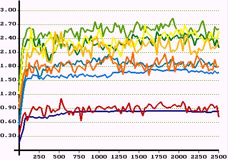
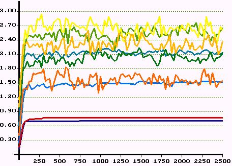
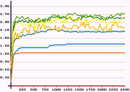
Figure 21. Average network dividend in all classes over 2500 periods. Top: first experiment. Middle: second experiment. Bottom: third experiment. Colours indicate classes.

4.24

The fact that finding a partner makes an agent better off is a trivial truth in our simulated world. But who gains what? An agent neither giving nor getting help in any of the 4 support games with his neighbours receives the payoff:

.

[8]

Obviously, the lower p_i, the higher . Let be the total payoff for a member of class i in period t. Then:

[9]

is what a member of class i gets in period t due to successfully established support relations. Let's call the network dividend. Figure 21 shows the development of the average network dividend for all 9 classes over 2500 periods for the three experiments.

4.25

The decisive point about the network dividend is that obviously the winners are in neither the best nor the worst risk classes. The winners are those in intermediate risk classes. In consequence, despite the class segregation accompanying the evolution of the network, equality (measured by the Lorenz curve or the Gini coefficient) increased in all three experiments.^[16] At the same time, the total wealth expressed in terms of aggregated payoffs increased as well.

4.26

The model shows at least five interesting effects:

• Even in a world of rational egoists with unequal endowments, support networks can evolve.
• These networks will be characterised by some class segregation.
• For intermediate classes, it is easier , comparatively speaking, to find partners for mutual support. In terms of network dividend those in intermediate neediness classes are the winners.
• The wider the range of classes whose members could establish functioning support relations among each other the higher the frequency of individuals dissatisfied with their network position.
• With the evolution of support networks and despite the accompanying class segregation, the equality of the payoff distribution increases.

4.27

One might summarise the situation rather provocatively: rational egoism, class segregation, increasing equality and increasing wealth go hand in hand. Nevertheless, as the chances of finding more attractive partners become better, more people will end up dissatisfied even with higher payoffs - at least in our model. The latter point has to be stressed since we did not address the question of empirical adequacy at all.

Why CA Based Modelling and Simulations?

5.1

The foregoing examples were presented to provide some evidence that CA based modelling is a fruitful approach to the understanding of social dynamics. Locality, overlapping neighbourhoods, and repeated interaction are properties of a significant class of dynamic social processes. CA based models include those features and are particularly well suited to contribute to a better understanding of micro/macro relations. However, they also have additional advantages:

• The macro effects in CA based models are often good examples (and sometimes even paradigmatic cases) of unintended consequences in social action. In Schelling's models, individuals do not intend to live in completely segregated areas. Nevertheless, that is where they end up living. In the support network model described above, individuals are interested in maximising their utilities and not in segregation (or increasing overall equality). But the latter effects are exactly what they produce by their maximising behaviour. Thus, CA based modelling can contribute to a better understanding of unintended consequences.
• Using CA based models of "artificial" worlds, it will often be possible to produce both quantitative explanations and predictions. But one can use these to learn about the "real" world as well. What can often be taken away from CA models might be called qualitative understanding of mechanisms. For instance, analysts finding racial segregation of neighbourhoods without racist neighbourhood preferences of their inhabitants could try to explain their findings via Schelling's segregation model. At the same time analysts may get an increased confidence in their findings if they are supported by results in an artificial world which is "similar enough". (Obviously a great deal of methodological work is yet to be done in order to clarify concepts like "similarity", "qualitative understanding", "stylised facts" etc. These concepts are widely used. But our understanding of them has remained intuitive and poor. It is a pity that philosophy of science has not yet discovered modelling and simulation as a frontier of methodological research.)
• The CA approach does not exclude centralised institutions in the model. For example, one might have an institution providing certain kinds of common knowledge about what is going on in the world. CA based modelling is therefore flexible enough to allow for narrow or wide definitions of locality and provides a natural framework for studying social self-organisation and corresponding political or economic manifestations based on the "invisible hand" paradigm. According to that paradigm, individuals acting in a more or less self-interested way will nevertheless produce desirable collective results on the macro level. Since that claim is a hypothesis and not an a priori truth, CA based modelling is an important framework for basic research on a fundamental question about societal organisation (Epstein and Axtell 1996, Guenther et al. 1997).
• Just as the CA approach may demonstrate unintended consequence for individuals, it may also indicate to researchers the surprising and previously unsuspected consequences of their theoretical assumptions. In general, our deductive capabilities are not that good. This becomes crucial when we are trying to understand processes in which numerous agents interact repeatedly. Since modelling these dynamic processes requires complex and numerous calculations, simulation is a useful deductive method for exploring the consequences of our theories. Simulation results can be related to existing empirical knowledge, they can stimulate new empirical studies and suggest theorems which can then be proved by analytical means. Modelling and simulation are therefore appropriate tools both for exploring current theoretical assumptions and developing new theories.
• CA based modelling also provides a convenient modelling environment for analysing the effects of different microfoundations in human decision making. It is possible to compare agents making use of adaptation and learning with those which are more rational, calculative and anticipatory (Flache and Hegselmann 1998). We can also compare agents with egoistic and altruistic preferences.
• In CA based models, one finds an inherent "spirit of simplicity" when approaching complexity. With regard to social applications, the subjects of analysis may be single elementary social interactions and mechanisms: looking for attractive partners, deciding to cooperate or defect, undergoing mutual influence, or finding a neighbourhood which meets certain requirements. Models of this type are totally different from "climate" models, where numerous different mechanisms and modules interact and interfere. "Thick models" (Kliemt 1996) like this make sense only if all their components are sufficiently well understood. Such models therefore tend to be found in more mature sciences and not usually in the social sciences.^[17] CA based modelling allows us to focus on the dynamics of elementary social interactions. Given the modest state of the art in the social sciences, CA based modelling seems to be an appropriate approach.

Notes

¹ A short and well written introduction to CA is provided in Casti (1992, volume 1, chapter 3).

² The model is basically a special case of French (1956), Harary (1959) and Abelson (1964). See also Nowak et al. (1990) and Hegselmann et al. (1998).

³As states we use a finite number (n) of real valued opinions. It would be just as easy to represent opinions by integer values but this would not affect any of the arguments presented in the paper.

⁴Obvously, the step functions in Figure 3 are not the only method for obtaining a finite number of possible opinions from an infinite set of real valued opinions. For example, it might be more realistic to assume that a particular opinion is adopted with a probability that declines with the distance between that opinion and u_i^*(t+1). However, we do not investigate this possibility, because this paper focuses on illustrating the CA framework rather than demonstrating the empirical adequacy of a particular model.

⁵That includes the possibility of modelling and understanding micro/macro feedback loops within the CA framework.

⁶For a discussion of artefacts related to updating procedures see Huberman and Glance (1993) and Hegselmann (1996).

⁷This model plays an important role in Lehman (1977), an early introduction to computer simulations for social scientists.

⁸ Another early application of checker board modelling is Hägerstrand (1965) where it is used to analyse the diffusion of new agricultural techniques.

⁹This is due to the fact that those models ask for a great deal of iterated computation even if very simple assumptions are used. It has become progressively easier since user-friendly programming languages and powerful debugging tools have been created. Nowadays corresponding hardware and software is also available to social scientists.

¹⁰ For recent overviews of research on social dilemmas see Schulz et al. (1994) and Liebrand and Messick (1996).

¹¹ The model was originally developed in Hegselmann (1994a, 1994b).

¹² In what follows, it is always assumed that D < M. When D > M we get support games in which those in need of help are those with favourable opportunities which they cannot take advantage of without support from another actor.

¹³ But notice that there are also many other equilibria.

¹⁴ The proof of [6] only exists as a manuscript available from the author.

¹⁵ This implies that we can assume that the equilibrium selection problem has been solved!

¹⁶ Details will be demonstrated in another article.

¹⁷ For an analysis of different types of simulations see Hartmann (1996), Kliemt (1996) and Troitzsch (1998).

References

ABBOTT, E A (1987) [1884] Flatland: A Romance of Many Dimensions. Penguin: Harmonsdworth.

ABELSON, R P (1964) Mathematical Models of the distribution of attitudes under controversy. In: N. Frederiksen and H. Gulliken (eds.) Contributions to mathematical psychology. Holt, Rinehart and Winston: New York, NY. pp. 142-160.

ALBIN, P S (1975) The Analysis of Complex Socioeconomic Systems. Lexington Books: London.

ALBIN, P S (1998) Barriers and Bounds to Rationality: Essays on Economic Complexity and Dynamics in Interactive Systems. Princeton University Press: Princeton, NJ.

AXELROD, R (1984) The evolution of cooperation. Basic Books: New York, NY.

BRUCH, E (1993) The evolution of cooperation in neighbourhood structures. Manuscript, Bonn University.

BURKS, A W (1970) Essays on cellular automata. University of Illinois Press: Urbana, IL.

CASTI, J L (1992) Reality rules: Picturing the world in mathematics , Volume I: The Fundamentals, Volume II: The Frontier. John Wiley and Sons: New York, NY.

DEMONGEOT, J, GOLES, E and TCHUENTE, M (eds.) (1985) Dynamical systems and cellular automata. Academic Press: London.

EPSTEIN, J M and AXTELL, R (1996) Growing Artificial Societies: Social Science from the Bottom Up. MIT Press: Cambridge, MA.

FRENCH, J R P (1956) A Formal Theory of Social Power. Psychological Review 63. pp. 181-194.

FLACHE, A and HEGSELMANN, R (1997) Rational vs. adaptive egoism in support networks - How different micro foundations shape different macro hypotheses. In: Leinfellner, W and Köhler, E (eds.) Game Theory, Experience, Rationality. Kluwer: Dordrecht. pp. 261-275.

FRIEDMAN, J W (1986) Game theory with applications to economics, second edition 1991. Oxford University Press: Oxford.

GAYLORD, R J and D'ANDRA, L (1998), Simulating Society: A MATHEMATICA Toolkit for Modelling Socioeconomic Behavior. Springer: New York, NY.

GUENTHER, O, HOGG, T and HUBERMAN, B A (1997) Market organizations for Controlling Smart Matter. In: R. Conte, R. Hegselmann and P. Terna (eds.) Simulating Social Phenomena. Springer: Berlin. pp. 241-257.

GUTOWITZ, H (ed.) (1991) Cellular automata: theory and experiment. MIT Press: Cambridge, MA.

HÄGERSTRAND, T (1965) A Monte Carlo approach to diffusion. European Journal of Sociology 63. pp. 43-67.

HARARY, F (1959) A Criterion for Unanimity in French's Theory of Social Power. In: D. Cartwright (ed.) Studies in Social Power. Institute of Social Research, University of Michigan: Ann Arbor, MI. pp. 168-182.

HARTMANN, S (1996) The world as a process: Simulations in the natural and social sciences. In: R. Hegselmann, U. Mueller and K. G. Troitzsch (eds.) Modelling and simulation in the social sciences from a philosophy of science point of view . Kluwer: Dordrecht. pp. 77-100.

HEGSELMANN, R (1994a) Zur Selbstorganisation von Solidarnetzwerken unter Ungleichen - Ein Simulationsmodell. In: K. Homann (ed.) Wirtschaftsethische Perspektiven I - Theorie, Ordnungsfragen, Internationale Institutuionen. Duncker and Humblot: Berlin. pp. 105-129.

HEGSELMANN, R (1994b) Solidarität in einer egoistischen Welt - Eine Simulation. In: J. Nida-Rümelin (ed.) Praktische Rationalität - Grundlagen und ethische Anwendungen des rational choice-Paradigmas. Walter de Gruyter: Berlin. pp. 349-390.

HEGSELMANN, R (1996) Cellular automata in the social sciences: Perspectives, restrictions and artefacts. In: R. Hegselmann, U. Mueller and K. G. Troitzsch (eds.) Modelling and simulation in the social sciences from a philosophy of science point of view . Kluwer: Dordrecht. pp. 209-234.

HEGSELMANN, R, FLACHE, A and MÖLLER, V (1998) Solidarity and Social Impact in Cellular Worlds - Results and Sensitivity Analyses. In: R. Suleiman, K. G. Troitzsch and N. Gilbert (eds.) Social Science Microsimulation: Tools for Modeling, Parameter Optimization and Sensitivity Analysis. Springer: Berlin 1998, to appear.

HUBERMAN, B A and GLANCE, N S (1993) Evolutionary Games and Computer Simulations. Proceedings of the National Academy of Science 90. pp. 7716-7718.

KEENAN, D C and O'BRIEN, M J (1993) Competition, Collusion, and Chaos. Journal of Economic Dynamics and Control 17. pp. 327-353.

KIRCHKAMP, O (1994) Spatial evolution of automata in the prisoners' dilemma. Manuscript, Bonn University.

KLIEMT, H (1996) Simulation and rational practice. In: R. Hegselmann, U. Mueller and K. G. Troitzsch (eds.) Modelling and simulation in the social sciences from a philosophy of science point of view . Kluwer: Dordrecht. pp. 13-28.

LEHMAN, R S (1977) Computer simulation and modeling: An introduction. Lawrence Erlbaum Associations: Hillsdale, NJ.

LIEBRAND, W B G and MESSICK, D (eds.) (1996) Frontiers in Social Dilemmas Research. Springer: New York, NY.

MESSICK, D M and LIEBRAND, W B G (1995) Individual heuristics and the dynamics of cooperation in large groups. Psychological Review 102. pp. 131-145.

NEUMANN, J von (1966) Theory of self-reproducing automata , edited and completed by Arthur W. Burks. University of Illinois Press: Urbana, IL.

NOWAK, A, SZAMREZ, J and LATANÉ, B (1990) From private attitude to public opinion - Dynamic theory of social impact.Psychological Review 97. pp. 362-376.

NOWAK, M A and MAY, R M (1992) Evolutionary games and spatial chaos. Nature 359. pp. 826-829.

NOWAK, M A and MAY, R M (1993) The spatial dilemmas of evolution. International Journal of Bifurcation and Chaos 3. pp. 35-78.

SAKODA, J M (1949) Minidoka: An analysis of changing patterns of social interaction. Unpublished doctoral dissertation, University of California: Berkeley.

SAKODA, J M (1971) The checkerboard model of social interaction. Journal of Mathematical Sociology 1. pp. 119-132.

SCHELLING, T (1969) Models of segregation. American Economic Review 59. pp. 488-493.

SCHELLING, T (1971) Dynamic models of segregation. Journal of Mathematical Sociology 1. pp. 143-186.

SCHULZ, U, ALBERS, W and MUELLER, U (eds.) (1994) Social Dilemmas and Cooperation. Springer: Berlin.

TAYLOR, M (1987) The possibility of cooperation . John Wiley and Sons, London.

TOFFOLI, T and MARGOLUS, N (1987) Cellular automata machines: A new environment for modeling. MIT Press: Cambridge, MA.

TROITZSCH, K G (1998) Multilevel modeling in the social sciences - Mathematical analysis and computer simulation. In: W. B. G. Liebrand, A. Nowak and R. Hegselmann (eds.) Computer Modeling of Social Processes. Sage: London.

WOLFRAM, S (1984) Universality and complexity in cellular automata. Physica D. 10. pp. 1-35.

WOLFRAM, S (ed.) (1986) Theory and applications of cellular automata. World Scientific: Singapore.

Return to Contents of this issue

© Copyright Journal of Artificial Societies and Social Simulation, 1998