Equation-Based Versus Agent-Based Models: Why Not Embrace Both for an Efficient Parameter Calibration?

and
Universidade de São Paulo, Brazil
Journal of Artificial
Societies and Social Simulation 26 (4) 3![]()
<https://www.jasss.org/26/4/3.html>
DOI: 10.18564/jasss.5183
Received: 08-Feb-2022 Accepted: 10-Jun-2023 Published: 31-Oct-2023
Abstract
In this work, we propose 2LevelCalibration, a multi-stage approach for the calibration of unknown parameters of agent-based models. First, we detail the aspects of agent-based models that make this task so cumbersome. Then, we conduct extensive research on common methods applied for this purpose in other domains, highlighting the strong points of each approach that could be explored to efficiently calibrate the parameters of agent-based models. Finally, we present a multi-stage method for this task, 2LevelCalibration, which benefits from the simplicity of equation-based models, used to faster explore a large set of possible combinations of parameters and to quickly select the more promising ones. These values are then analysed more carefully in the second step of our method, which performs the calibration of the agent-based model parameters' near the region of the search space that potentially contains the best set of parameters, previously identified in our method. This strategy outperformed traditional techniques when tested to calibrate the parameters of an agent-based model to replicate real-world observations of the housing market. With this testbed, we show that our method has highly desirable characteristics such as lightweight implementation and consistency, which are ideal for agent-based models' development process.Introduction
Agent-based models are a valuable tool for modeling complex systems by allowing the representation of the heterogeneity in the constituents parts of a system (Dilaver & Gilbert 2023). This level of disaggregation makes the analysis of emergent behaviours and second-order effects possible, in opposition to traditional top-down modelling that can hardly capture them (Van Dyke Parunak et al. 1998). Such appealing characteristic make them very common in domains that study the consequences of human systems, such as Economics (Hamill & Gilbert 2015; Tesfatsion & Judd 2006), Social Sciences (Borrill & Tesfatsion 2011; Retzlaff et al. 2021; Squazzoni 2010) and Epidemiology (Hunter et al. 2017; Marshall & Galea 2015).
The most prominent characteristic of agent-based models is nonetheless one of its main impediments for a widespread adoption. To validate a model, typically we compare the output of the simulation against real-world data. This is an obstacle for agent-based models for the following reasons: (i) usually we have access only to surveys, census and the results of aggregated data, which cannot bring the complete information required to model the individual behaviour of the agents in the system; (ii) as agent-based models are commonly used in the realm of human systems, mental processes, feelings and expectations are frequent concepts adopted in the models, despite the impossibility of objectively measuring and attributing a precise numerical representation to them. The process of calibrating unknown model parameters is hence a vital step on the validation process of those who adopt an agent-based approach, as many of the parameters required for the simulation should be estimated from an incomplete and limited set of data observed from a real-world phenomenon (Moss 2008).
The task of parameter calibration can present several degrees of difficulty, varying from satisfactorily applying simple linear regression to exploring huge and rough search spaces. Unfortunately, agent-based models parameter calibration is usually closer to the latter, mostly due to its own structure. The decision process that governs agent behaviour can be as detailed as desired, so frequently we are faced with large search spaces, as each parameter to be calibrated increases in one dimension this search space. Additionally, the surface that must be explored to find the most probable set of parameters is rugged, with plenty of local minimums and maximums resulting from the non-linear relationship among the parameters. As if it was not enough, frequently the output of the simulation is non-deterministic due to the inherent randomness of the model, which might make the process of assessing the likelihood of a set of parameters even more difficult.
As the calibration of parameters in an agent-based model is a crucial, yet remarkably challenging task (Banks & Hooten 2021), in this work we propose a new strategy for this purpose, tailored to the idiosyncrasies of agent-based models while making use of the best practices applied in other modelling approaches.
The Challenge of Calibrating Parameters in Agent-Based Models
A model is an abstraction of reality as it performs a simplification of the real world that is good enough for its purpose (Robinson 2008; Zeigler et al. 2018). In essence, to build a model we should choose which aspects (input variables) we take into account, and how we define the relationship among such aspects. A system’s functioning can be described either mathematically or by computationally simulating the interaction of each system’s component. The first approach, also commonly called top-down, extracts the dependence between the selected input variables. This mathematical relation is expressed in an analytical form (i.e., by means of a mathematical equation), or can rely on numerical approximation methods that extensively sample the search space to estimate such relationship. In contrast, a computational model (or also a bottom-up model) does not require explicitly the definition of a mathematical formula; it relies on the modeling of the constituent parts of the systems and their interplay with the environment and other particles.
At first glance, it is clear that a computational model can be largely more expensive than an equation-based model, as it scales with the number of particles of the system that usually outnumber the input parameters of a mathematical model. However, there is extensive work that describe several situations in which a bottom-up modelling approach is beneficial (Van Dyke Parunak et al. 1998), especially when the behaviour of the system is governed by emergent phenomena and by the so-called second-order effects (Gilbert 2002), which is the property of the particles in the system to react to new emergent collective behaviours.
The core argument is that while one can calibrate the parameters of a mathematical model to replicate the past behaviour of the system and thus provide an estimation about its future behaviour, these forecasts will only keep their accuracy if the structure of the system remains stable over time. If relevant variables rearrange in such a way as to alter their coupling structure, or even if the impact of some variables is amplified in a non-linear fashion, the mathematical model might become useless. With an agent-based approach, on the other hand, one can better investigate the underlying behaviours that led to the observed phenomenon (or, as pointed out in Mauhe et al. (2023), to disclaim some beliefs). By doing so, such knowledge can be extrapolated, leading to many reconfigurations of the model to generate hypothetical yet plausible scenarios (what if scenarios) by altering the structure and stability of the system and generating unforeseen (and almost always counter-intuitive) forecasts. In this way, we can say that agent-based models have a higher power of expression, extremely desirable to replicate complex systems, that unfortunately makes, at the same time, the task of parameter calibration very cumbersome for the following reasons:
- Many parameters: With an agent-based model, there is no general formula that combines all the input variables to produce an output. The modeller describes the behaviour of the components (agents) and simulates their interaction to generate the resulting overall behaviour of the system, that is not visible (and not easily predicted) beforehand. This characteristic can foster an overparameterization of the model, as the modeller tries to put as many details as possible in order to replicate the desired but not yet visualized output of the system. A large number of parameters is not advisable in any modeling approach, as it provides a high degree of freedom to the model that might be more than necessary to describe the system: a model that requires a large number of inputs might be using them only to compensate its structural errors, and not to better approximate the target phenomenon (this situation is known as the numerical daemon, Gan et al. 2014).
Particularly, from a parameter calibration standpoint, a large number of variables is an obstacle as it brings along two undesirable conditions:
- Combinatorial explosion : to estimate the most likely set of parameters that generates the observed result, the parameter calibration method should vary all the parameters to explore a large set of possible combinations to evaluate what are the most probable ones. Intuitively, it is clear that an increase in the number of variables also increases the number of combinations that should be assessed. Mathematically speaking, each new parameter increases one dimension in the search space. To keep the same sampling density, there should be an exponential increase in the number of samples for each added dimension. This property is also referred to in the literature as The Curse of Dimensionality (Banks & Hooten 2021);
- Equifinality: the property in which an observed output could have been generated by many different combinations of parameters. As parameter calibration methods are essentially estimating the probability of each set of parameters in generating the expected output, this condition can be misleading: once you have a large set of equally probable and plausible candidates, it gets harder to identify which is the correct one. Moreover, the method is more prone to find a spurious set of parameters that describe the overall expected behaviour of the system: the number of correlations is convex with the number of dimensions. By testing too many parameter combinations, we can find several ones that might fit remarkably well into the expected output, but only a small subset will represent the real correlations among input and output - and it is virtually impossible to differentiate between spurious and real correlated sets of parameters.
- Non-linear relations: agent-based models are notably used on strongly non-linear domains, such as human systems. We say that we have a nonlinear relation when the impact on the output is not proportional to the change on the input, meaning that even small perturbations can generate huge differences in the result. This promotes an almost erratic behaviour of the system, that makes it harder to be predicted. Parameter calibration methods rely on sampling strategies, that can vary each variable one at a time or several ones at once, aiming to account for how much difference in the output can be proportioned to an alteration in one variable. In linear systems, we can easily estimate the pattern of the gradient which leads to an optimal combination of parameters. In non-linear systems, the parameter estimation method should navigate a rough space, with gradients that suddenly change in direction and slope, resulting in local minimums and maximums. It is almost impossible to extract the importance of each parameter to the resulting behaviour of the system, and even more complex to certainly attribute the best value for an unknown parameter (somewhere in a little unexplored corner of the search space there can be a better combination of parameters as the search space surface does not present a monotonic behaviour).
- Stochasticity: agent-based models rely on representing the heterogeneous behaviour of the agents and on simulating its interactions. The same interaction performed by agents with different profiles can generate different results, which in turn can be reflected in the overall output. Moreover, such interaction among agents can occur by pure chance, depending, for instance, on the position of each agent on a grid or a network. Two executions of the simulation can thus provide different outputs, even if they are initialized with the same parameters. The inherent stochasticity of the model increases model error variance (Kinal & Lahiri 1983), bringing a new layer of uncertainty to parameter calibration methods, as they should account for changes in the overall behaviour due to modifications on the values of the parameters and due to the randomness of interactions of the agents.
- Domain of the parameters : usually agent-based models need to represent concepts that are better approximated by the family of Power Law probability distributions, such as stock market prices (Mandelbrot & Taylor 1967), wealth (Vermeulen 2018), epidemics (Cirillo & Taleb 2020) and wars (Cirillo & Taleb 2016), just to name a few. This fact occurs more often than commonly believed (Chen et al. 2022) and it brings important theoretical implications such as the possibility of infinite theoretical moments (mean, variance1 Fedotenkov 2020; Granger 1968), which violates most of the assumptions of traditional mathematical methods. Under heavy-tailed probability distributions, even when those moments exist, it can require a prohibitive number of samples to correctly estimate such properties, seriously compromising the convergence of traditional methods or even invalidating their outputs (Taleb 2020).
Model Parameter Calibration Techniques
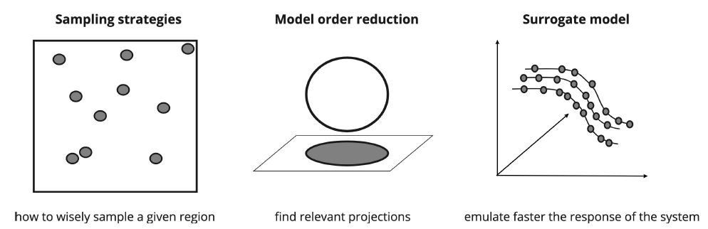
Parameter calibration is a classical mathematical problem, whose final objective is to find the set of parameters that minimize the difference between real and simulated data (Liu et al. 2017). It is part of a research area called Uncertainty Quantification, that encompasses problems such as uncertainty propagation, sensitivity analysis, and parameter calibration (also referred to as inverse problems when we also have uncertainty on the input variables). Located at the heart of all methods to solve uncertainty quantification problems there lies sampling strategies to explore an unknown search space that is not easily described by an analytical formula (Tarantola 2005). When dealing with intensive sampling tasks, we can adopt three strategies to reduce the computational burden of the task (Frangos et al. 2010), shown in Figure 1. Namely, they are:
- Improving sampling strategies, to extract more information from a given number of samples or demanding fewer samples positioned on strategic locations to properly cover the search space;
- Reducing the dimensions of the search space, by considering only a subset of the most important parameters, which as a consequence reduces the number of required samples;
- Constructing surrogate models, that are computationally cheaper to execute, thus decreasing the time to generate the output of a given number of samples.
There is extensive work from the research community to use one or a combination of strategies for uncertainty quantification, and to describe all of the strategies in detail is beyond the scope of this work. We refer the reader to Biegler et al. (2011), Sullivan (2015) for more details.
Sampling strategies
Sampling strategies are related to how the method for parameter calibration explores the search space collecting samples. These samples are used to determine some relevant properties of the search space, such as in what locations we have more chances finding the set of parameters that minimizes the error of the model compared against ground truth data. Better strategies focus on extracting more information on key regions of the search space to assure a faster convergence. However, those sampling methods should guarantee a good coverage of the search space, in order to find in the first place what regions should be explored more carefully. Sampling strategies are tightly coupled to the field of Design of Experiments (DoE), as they share the ultimate goal of optimizing the number of experiments to the most important ones (Lorscheid et al. 2012).
Sampling strategies can be used alone to reduce the computational cost of calibrating the parameters or they can be used in combination with the other two approaches (model order reduction and/or response surface creation). The most efficient sampling strategy can vary depending on the use case (Sullivan 2015).
The more naive sampling strategy is known as the Monte Carlo strategy, in which the values of each parameter are chosen randomly between its range of variation. There is no guarantee that the samples will be homogeneously distributed over the search space (there is a non-negligible chance that the samples are clustered among small subspaces) and, moreover, there is no guarantee that regions that potentially are more likely to contain a better set of parameters will be explored in more detail. As this is a simple method, with a very straightforward implementation, it is used as a benchmark for all other sampling strategies.
In order to overcome the undesired sampling clustering that might happen with Monte Carlo, some other techniques are adopted. Latin Hypercube is one sampling strategy commonly applied that relies on equally dividing the search space into a grid of cells, assuring that there is one sample on each of those cells (Shields et al. 2015). Essentially it comes in two different flavours: a pure Latin Hypercube, in which the sample should be within the borders of the cell, or the Full Factorial version2, in which each sample is extracted precisely from the borders of each cell, being equally distant from each other.
Quasi-Random Monte Carlo is another clustering-avoidance sampling strategy. It is based on the definition of an initial sample (chosen randomly) which will dictate what will be the next samples: they will be selected by following a numerical sequence that presents some mathematical properties (usually it is based on a Sobol’ sequence, Sobol 1990). As Latin Hypercube and Quasi-Random Monte Carlo are more space-filling than the traditional Monte Carlo method, they both present quicker convergence. However, they require more computational power to calculate where to position the samples, which could easily be a drawback in many situations (Kucherenko et al. 2015).
Importance sampling and Markov Chains, on the other hand, try to focus on fostering the sampling on regions of the search space with a higher potential to include a better set of parameters. With Importance Sampling, one can estimate an unknown distribution (in the case of parameter calibration, the likelihood associated to each set of parameters), while sampling from another, more tractable probability distribution, that we will refer to henceforth as the sampling probability distribution \(s\). Probability distribution \(s\) must be chosen so as to overweight a potentially interesting region by concentrating more samples on it. Because some regions of the subspace were favored by \(s\), a correction must be later applied to the samples in order to extract the real probability distribution. Choosing a good probability distribution \(s\) to sample from is key for the method performance as some can generate an expectation with an infinite variance - in this case, a pure Monte Carlo method would outperform Importance sampling (Owen & Zhou 2000).
The Monte Carlo Markov Chain is an umbrella term for several sampling techniques of multidimensional spaces. Unlike the Monte Carlo method, which considers a set of independent samples to estimate the unknown probability distribution, the Markov Chain method consists of extracting a chain of correlated samples that are generated by a walk over the search space (Brooks et al. 2011; Geyer 1991). As mentioned, there are several possible implementations of the Monte Carlo Markov Chain, and their subtle differences stem from the way a point in the search space is added to the chain of samples. The most adopted sampling strategy is the Metropolis-Hastings (Roberts & Smith 1994). It is based on the definition of an initial sample point, the choice of a sample candidate and analysis of acceptance/rejection of the new sample: the new sample is accepted if it presents a higher likelihood (in the case of parameter calibration, if it reduces the observed error of the model output when compared to real data); otherwise, the new sample is accepted with a random probability, even with a lower likelihood. This property assures that, in the long run, we have a satisfactory coverage of the whole search space, while at the same time emphasizing the search in potential hot spots.
Metaheuristics encompass techniques that tries to implement the trade-off between exploring a huge search space while focusing on subspaces that present a higher potential to contain at least local optimum solutions. Simulated Annealing resembles a Monte Carlo Markov Chain with a Metropolis-Hastings sampling strategy. The key difference is that while on Simulated Annealing the probability of accepting a sample with inferior likelihood is time-dependent(i.e., the probability decreases as more samples are chosen from the search space), with the Metropolis-Hastings this probability is strictly related to the likelihood of the new samples (the smaller the likelihood, the smaller the chance this sample is accepted). Genetic algorithm is a widespread metaheuristic that implements the metaphor of natural selection, fostering the exploration of regions of the search space which showed the greater potential of containing a good set of parameters. Metaheuristics in general present some draw-backs: first, they lack the mathematical formalism of sampling (Saka et al. 2016; Tarantola 2005); secondly, their performance is closely coupled to the chosen parameters that regulate their behaviour (for instance, the size of the parent population in Genetic Algorithms). The CMA-ES algorithm (Hansen 2006), which stands for Covariance Matrix Adaptation - Evolution Strategy, is a population-based metaheuristics, that takes advantage of second-order information and is a derivative-free method. It is based on a multi-variate normal search distribution, regulated by the covariance matrix that is continuously updated, and on evolutionary computation, by applying selection/ranking techniques over recombining generations. One of the great advantages of the CMA-ES method is that it can regulate its own parameters, such as step size, overcoming one of the great drawbacks of metaheuristic methods, as well as being a more agnostic method that does not rely on restrictive assumptions about the objective function.
Similarly, History matching systematically reduces the search space by evaluating if the set of parameters makes the model mimic important properties of the target system over time. The combination of parameters that do not successfully replicate those properties is removed from the search space, narrowing it for subsequent executions. To account for the intrinsic randomness of the model, a fixed number of executions with the same set of parameters is performed, and the evaluation is based on the mean and variability of the difference between the ensemble of simulations with the same parameters and the observed behaviour (Papadelis & Flamos 2019). History matching is widely used in the oil industry to model reservoir properties but is not limited to this domain (Vernon et al. 2014). Computational resources can be a barrier depending on the number of points analysed, model parameters and instances of the ensemble.3 Moreover, in high dimensional spaces, the method can be trapped on suboptimal solutions, resulting mistakenly in the discard of a viable set of parameters and even a complete region of the search space.
Gradient-based strategies also follow an approach to concentrate on regions of the search space with a combination of parameters that minimizes the error of the simulator output. They require the definition of a loss function (i.e., a function to evaluate how far the output of the simulation in which a set of parameters differ from real data). The gradient of each parameter, which represents how much the output responds to changes in its values, is computed for each iteration. Repeatedly, the method selects a combination of parameters that minimizes the loss function, until it eventually reaches the point of (local) minimum (Lu 2022). There are several methods to implement gradient-descent strategies, that vary on how to calculate the gradient and how to select the parameters’ values. The most prominent methods in this family are stochastic gradient descent (SGD) and Adam (Kingma & Ba 2014) optimizer. As with any method, they can have some undesirable behaviour, such as noisy and slow convergence (for SDG) (Ruder 2016) and problems of convergence (not theoretically guaranteed for Adam; Chen et al. 2018; Reddi et al. 2019).
Another approach some sampling strategies adopt is to increase the information extracted from samples. These sampling strategies do not try to reduce the number of samples to converge, but they apply techniques to converge more quickly, by combining samples generated by models with different accuracies and computational costs. This is a mixed strategy, as it relies both on (i) sampling wisely and on (ii) model-order reduction techniques or on the creation of response surfaces to generate models that perform faster at the expense of accuracy. There are essentially two strategies that can be put under this classification: Multi Level Monte Carlo and Bayesian Optimization.
Multi-Level Monte Carlo is based on the assumption that there are at least two models with increasing accuracy and consequently increasing computational cost. This method relies on the telescoping sum of the expectation, which requires only the computation of the difference in the accuracy between the models (Jasra et al. 2020). A finite number of samples (i.e., sets of combinations of the parameters being calibrated) is simulated both on the model with higher accuracy and on the lower accuracy model in order to properly calculate the accuracy difference. After this calculation, the method determines the number of required samples on each model to converge properly. Most of the samples are executed on the cheapest model, so Multi-Level Monte Carlo demands fewer computations to achieve the same results obtained from a pure Monte Carlo strategy.
Bayesian Optimization (Frazier 2018), as the name implies itself, heavily relies on Bayes Theorem. It has two key elements: a statistical model of the objective function (which in our case tries to minimize the error between the results obtained from the simulation model against ground truth data), and an acquisition function that determines where to sample on the next iteration. The first step collects a fixed number of samples that will be used by the statistical model (commonly Gaussian Process) to generate a surrogate of the objective function. The statistical process provides the most probable function that interpolates the samples, with an associated confidence interval. The acquisition function then estimates the next sample to be collected, which should be the one located in the region of lower confidence, therefore maximizing information brought by this new sample. The whole process of fitting the statistical model is then triggered again, generating a new surrogate of the objective function and consequently the region with higher uncertainty, that will be explored with the next sample. This iteration stops once a predefined condition is reached (computational time, level of confidence, error). For an extensive list of references about Bayesian optimization and its application to demography modelling, we refer the reader to Bijak (2022).
Model-order reduction
It is very intuitive to infer that models that receive fewer input parameters are executed faster, as fewer calculations are required to generate the output. Additionally, such models require a substantially reduced parameter combinations to be calibrated (remember that the number of required samples increases exponentially with the number of parameters). Therefore one good approach is to find which ones dominate system response. The task of sensitivity analysis (Oakley & O’Hagan 2004), or feature selection on Machine Learning (Chandrashekar & Sahin 2014), does precisely this job, as it aims at identifying which input parameters contribute most to output variations (Saltelli et al. 1999). There are two common approaches when performing a sensitivity analysis: local and global sensitivity analysis methods. The first one varies one parameter at a time, while all others are fixed. The latter one varies all parameters at the same time, which allows a more comprehensive analysis of the consequences of parameters variations by also observing the impact on the interaction among the parameters in the overall response.
Within the local approach, the most naive strategy is based on the calculation of correlation metrics between the input parameter and the output of the system. Those metrics include Pearson or Spearman correlation, mutual information, among others. In the same category, Differential Sensitivity Analysis extracts the partial derivatives of each parameter to infer its relevance.
As global sensitivity analysis methods are more computationally expensive, often a multi-stage approach is preferred: screening methods selects a small yet representative subset of parameters, that will be evaluated more carefully. Such methods do not measure the importance of each parameter in a numerical form but essentially indicate comparatively which ones contribute most to the system’s behaviour. The Principal Component Analysis (PCA) technique is applied recurrently to this end. In general terms, it employs mathematical transformations to extract an independent set of parameters (the principal components) among an extensive list of parameters (Jolliffe & Cadima 2016). PCA methods have some caveats: they are based on the Gauss-Markov assumption, which might not be fulfilled if data is not normally distributed (Taleb 2020). Similarly, some works opt for stepwise regression in order to find out what are the most impactful input parameters, by adding or removing an input variable to observe the consequence on the accuracy of the model’s output. A parameter is considered relevant if the accuracy decreases more than a predetermined level of acceptance or if it is considered statistically relevant for the output. Unfortunately, this method is unsuitable for scenarios with a large number of parameters, as due to the phenomenon of equifinalitity, it increases the chance of finding misleading answers (Smith 2018).
The Morris method, also sometimes called as One-at-a-Time method, might be inadvertently classified as a local method, but in fact, performs much more a global analysis. It creates a vector with all the input parameters and sequentially alters only one value of the vector at a time, for a fixed number of steps, generating a trajectory. After generating several trajectories, the method calculates certain statistics for each parameter, such as mean and standard deviation to summarize the importance to the system’s output (Morris 1991). Fourier amplitude sensitivity test (FAST) is a long-term well-established method for sensitivity analysis, that decomposes the variance of model output by applying a Fourier transformation, and then sampling suitably to compute the importance measure of each parameter (Reusser et al. 2011; Saltelli & Bolado 1998).
Similarly, ANOVA, which stands for Analysis of Variance, adopts techniques developed on the field of Design of Experiments (DoE), decomposing the variances into partial ones, that are later and incrementally expanded by increasing their dimensionality (Gelman 2005; Speed 1987). Sobol’ indices, often called Variance-based sensitivity analysis, relies on the ANOVA decomposition of functions (Owen et al. 2014) and the Monte Carlo method4 to calculate how each parameter contributes proportionally to the overall output, as well as the effect on the output generated by the interplay among parameters. It essentially measures the importance of subsets of parameters, and then incrementally and hierarchically decomposes each subset into multiple one-variable sets in order to calculate its unitary importance. Sobol’ indices is the only one that escapes from the curse of dimensionality, by implementing the Total Sensitivity Index, which clusters the variance of several variables into a unidimensional value, that is later decomposed into each of the constituent variables (Ratto & Saltelli 2002). However, this method still requires several executions of the model to properly calculate its index, which might compromise its usage with heavy simulation models (Lamboni et al. 2013)5 and, more importantly, it can only be applied when the variables present a finite variance (Brevault et al. 2013), which might not be naively assumed, especially in social domains.
Surrogate models
Surrogate models are also sometimes referred to as response surface, emulators or metamodels6. They try to faster replicate the output of a simulation model (the response surface of the model), without implementing its process dynamics. Response Surface Methodology (RSM) is aimed at extracting an unknown (usually nonlinear) function that describes the relationship among independent predictor (or input) variables. In essence, to create a response surface one needs to perform a numerical approximation that relies on experimental strategies to explore the space of parameters and estimate an empirical relationship with the output of the model (Myers et al. 2016).
The task of constructing a response surface can be preceded by an optional screening step, often referred to as step zero, which consists of performing screening on input variables to identify which ones influence most the shape of the surface. It is essentially the strategy employed on the aforementioned model-order reduction.
The techniques employed to construct such response surfaces vary according to certain characteristics of the process that governs the model’s behaviour it is trying to replace. For a simpler process, polynomials can satisfactorily describe the surface, but this is not the usual scenario, which requires the usage of more sophisticated methods. Gaussian Processes have been successfully applied to perform regressions on stiff search spaces. In essence, while traditional regression methods try to find the best parameters that fit a predefined (linear or nonlinear) function, Gaussian Processes explore a wide range of functions that could describe the training set always considering the assumption that data stemmed from a multivariate (usually Gaussian) distribution (Ebden 2015). In order to make this task computationally tractable, the range of variation of all variables should be defined. Moreover, a Gaussian Process assumes that nearby input values will generate close outputs in the response surface (Williams & Rasmussen 2006). This relation is described by a covariance matrix, that can be extracted from the training data, but still, the user should specify the mean of such correlation matrix, and the kernel of the shape of the correlation, which is usually assumed to be a Gaussian. The definition of the covariance function predominantly determines the reliability of the regression made by the Gaussian Process (Ebden 2015). Correctly executing a Gaussian Process regression is very time consuming and computationally expensive7. Additionally, it can be a useless effort as this method heavily relies on the variance of involved variables that might not exist8 (Nair et al. 2013). We refer the reader to Kennedy & O’Hagan (2001) for an interesting use of Gaussian Process to model and propagate several sources of uncertainty of calibrated computer models Conti et al. (2009), Oakley & O’Hagan (2002) and to construct an emulator for sensitivity analysis.
Machine Learning techniques, especially unsupervised algorithms, have been broadly adopted to generate response surfaces because they have the power to model rough surfaces without requiring much prior knowledge of the target surface. Neural networks are nowadays undoubtedly the most widespread approach for such task, presenting impressive results on extremely challenging scenarios, such as chaotic systems (Lamamra et al. 2017) and processes strongly governed by differential equations (Meng et al. 2020). They are not a panacea, though. To implement a neural network several definitions must be made beforehand or on a trial-and-error approach. Such definitions include the network architecture, the shape of the activate functions of neurons, the learning rate and the loss function. Moreover, the size and quality of the training set are key for the success of the task of generating a surrogate model based on neural networks. It is broadly known that neural networks are good at interpolating, not extrapolating the search space (i.e., going beyond the training domain, as it relies on the universal approximation theorem; Barron 1993; Schäfer & Zimmermann 2006). This means that the samples should cover to some extent all the characteristics of the search space, demanding a huge amount of data to this end. Additionally, there is a known drawback of disproportional importance given to regular, ordinary samples (that are more common and, consequently, more abundant in the training dataset) during the learning phase than non-frequent samples resulting from the combination of input variables with extreme values, amplified by strongly non-linear relations9. This question is addressed in the literature as imbalanced training samples (Hensman & Masko 2015).
A multi-step approach can be adopted for the construction of response surfaces. The first step consists of estimating the shape of the response surface (for instance, the location of maximums and minimums) to identify which regions of the search space possibly lie close or far from the optimum. In essence, it performs an approximation of the effect of input parameters on the response. This first-level response surface is then used as the building block of a method responsible for an improvement, which searches for (at least local) optimum regions. Steepest ascent/descent is generally the method of choice for this purpose. In phase two, a more intense exploration nearby the selected region takes place, and a second-order response surface is built, better approximating the curvature of a small region near the optimum.
For a discussion about some of the surrogate construction techniques for agent-based models, we refer the reader to Banks & Hooten (2021).
Model parameter calibration in ABM
Agent-based models are valuable tools for the simulation of complex systems, especially to deepen our understanding of systems’ dynamics and to substantiate policy-making decisions. Comparing their ability to replicate real-world data is an important requirement to provide supporting evidence of the value of such models. Surprisingly, parameter calibration is performed by only a minority of work published in this area (some studies suggest something near to 10%, Thiele et al. 2014). One of the possible reasons for this scenario could be due to the technical complexity required by the task of parameter calibration of agent-based models, which makes it essential to define efficient methods for this purpose (Banks & Hooten 2021).
We performed extensive research to identify what techniques have been adopted in the literature, concerning agent-based parameters’ calibration. Overall, such techniques are frequently selected without entering too much into the model and data idiosyncrasies. We provide a summary of this research in Table 1, highlighting canonical techniques and giving minor details about the implementations in the footnotes.
| Reference | Sampling | Model-order reduction | Surrogate model |
|---|---|---|---|
| Lamperti et al. (2018) | Quasi-random (Sobol’)10 | No | Machine Learning11 |
| Papadopoulos & Azar (2016) | No | No | Linear Regression |
| van der Hoog (2019) | No | No | Machine Learning12 |
| Grazzini et al. (2017) | Monte Carlo Markov Chain | No | No |
| Barde & van der Hoog (2017) | Latin Hypercube13 | No | Gaussian Process |
| Venkatramanan et al. (2018) | Bayesian Optimization | No | No |
| Zhang et al. (2020) | Importance sampling14 | No | Machine learning15 |
| Lux (2018) | Importance sampling16 | No | No |
| Fonoberova et al. (2013) | Latin Hypercube | Variance-based | Machine Learning17 |
| Garg et al. (2019) | No | Regression18 | Regression19 |
| McCulloch et al. (2022) | History matching20 | Latin Hypercube | No |
| Kotthoff & Hamacher (2022) | Gradient-based21 | No | No |
Some work try to summarize and discuss different approaches for parameter calibration, such as Reinhardt et al. (2018)22, Fagiolo et al. (2019) and more recently Carrella (2021). It is very unlikely that there is a silver-bullet, one-size-fits-all solution for agent-based parameters’ calibration, as such models are applied in a myriad of domains, with diverse data aggregation and parameters’ dependence.
2LevelCalibration: A Multi-Stage Approach for Agent-Based Models’ Parameter Calibration
By analysing both theory and previous work, we can infer that the construction of surrogate models can be very beneficial, as they can substantially spare computational resources when adopted in combination with effective sampling strategies (especially Multi-Level Monte Carlo and Bayesian Optimization). The most traditional and agnostic23 method for the construction of surrogate models, Machine Learning is nonetheless also very time-consuming as it requires a large number of samples and several configuration decisions. If the surrogate development is coupled with model-order reduction techniques, the burden of this process also increases sharply.
One can argue that the process of constructing a surrogate model is performed only once or a few times, depending on the strategy adopted. Notwithstanding, this argument misses an important aspect of the agent-based modelling process: such models inherently present a high level of epistemic uncertainty (Sullivan 2015), which is the one associated with how much one knows about a target process. This epistemic uncertainty can be attributed both to model uncertainties (in which we do not even know if the model correctly describes the target phenomenon) and to parametric uncertainty (in which we assume that the model is correct but there is some uncertainty on the values of the parameters). With an agent-based approach, the modeller does not have visibility about the output before executing the model – and to execute the model, several parameters should be calibrated. Consequently, the parameter calibration process is repeated several times during the phase of model development, as the modeller tries to explore and, even more important, to evaluate the performance of several assumptions regarding the agent’s behaviour and cooperative structures. So, with an agent-based approach, model and parameter uncertainty are intrinsically related: while testing the model’s assumptions, we should use parameter calibration techniques that are both efficient and that present consistent results.24 In other words, we aim for techniques that are lightweight (since the calibration step is performed repeatedly) and that have good convergence (i.e., if there is an optimal set of parameters that can fit the model, the technique should be able to find a solution within a small deviation). Hence efficiency and consistency are requirements that should be satisfied by our proposed approach 2LevelCalibration.
The most appealing methods that meet our desired requirements take advantage of the combination of a large pool of executions from low-cost models and a few ones from costly and most accurate models, which demands the development of surrogate or reduced-order models. To construct low-cost models affordably for agent-based systems, we propose the usage of a Model Library. This idea is grounded on the concept that the micro-behaviour of the particles of a system, described by many factors and interactions, can lead to behavioural patterns at a macro-scale (Grimm et al. 2005; Siegenfeld & Bar-Yam 2020).
Specifically in agent-based models for social simulation, it is common to obtain only a time series that portrays system dynamics over time. Thereafter, most commonly the surrogate model should describe an evolving dynamic system, that is governed by ordinary differential equations (ODEs), that can be adopted as a surrogate of an agent-based model. We chose ODEs to compose our Model Library according to work developed in the research area of System Dynamics (SD). Sterman (2000) identified the fundamental behavioural modes of social dynamic systems, described as the most common recurrent patterns in this domain, with the advantage of relying on the definition of very few parameters. As a byproduct of this strategy, our method performs, at no cost, a model-order reduction, while simultaneously avoiding the Curse of Dimensionality by making model evaluations independent on the number of parameters of the agent-based model. Moreover, by successfully identifying the key parameters of the system dynamics to generate the surrogate model, we are more likely to develop robust models that are both representative of the target system’s current conditions and of possible regime shifts (Grimm & Berger 2016).
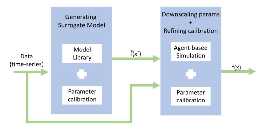
The process of reducing the number of parameters by collapsing several parameters into one requires a later step of downscaling. This step translates the aggregated value into the multiple parameters of the agent-based model that are merged into the higher level parameter of the ODE. For this reason, our method relies on a second phase for calibrating the agent-based model’s parameters. In fact, our method 2LevelCalibration can be seen as a multiscale approach, an effective strategy for complex systems because they have the property of presenting simultaneously different patterns of behaviours at different scales (Grimm et al. 2005). In the first step, the ODE surrogate function \(\hat{f}\), which requires a smaller number of parameters than the original model, is generated and calibrated using ground-truth data. In the second phase, the reduced set of parameters calibrated previously is used as initial values. The whole set of parameters is then calibrated, but now comparing the result of the original agent-based model, i.e., function \(f\), against ground-truth data. Figure 2 denotes this process.
The choice for using System Dynamics’ fundamental models brings also a key advantage on the task of going back from the macro parameters provided by the surrogate modelling to the micro ones, required by the agent-based model. To date, there is no systematic silver-bullet method to interconnect aggregated variables (the macro parameters of the ODE) and their constituents components (the micro parameters of the agent-based model), and this is precisely the fact that makes agent-based models so useful. However, System Dynamics relies on the assumption that it is possible to infer a system’s structure by observing its output. In a nutshell, in Systems Dynamics (SD), the structure is composed of two basic units: accumulators (represented by stocks) and flows, coupled to feedback loops that provide the dynamic character of the system (i.e., its property of changing over time) (Forrester 1994). By taking advantage of the types of structures described in SD that give rise to the observed output, the modeller can intuitively group parameters that supposedly contribute to the observed dynamics. This strategy does not provide a formal technique for grouping parameters, but it is easier for the modeler to make an educated guess.
By executing the first step of parameter calibration over function \(\hat{f}\) (the surrogate model), with a reduced number of parameters, we are able to explore the whole search space faster, identifying hot spots more easily and facilitating the second step that is initialized with more favourable conditions. We believe that this extensive coverage is especially determinant for providing the desired consistency in our method. Furthermore, our method is less likely to be trapped on local minimums with a suboptimal configuration of the values of the parameters. The characteristics of the search space of the parameters of an ODE are largely more tractable than one of the agent-based model parameters. First, because a space with lower dimensionality is easier to explore, and second because of the nature of the parameters that need to be calibrated: their range of variation and their variability are smaller (sometimes orders of magnitude smaller). Additionally, estimating the initial values is smooth - they just need to allow the ODE to describe the expected stylized shape.
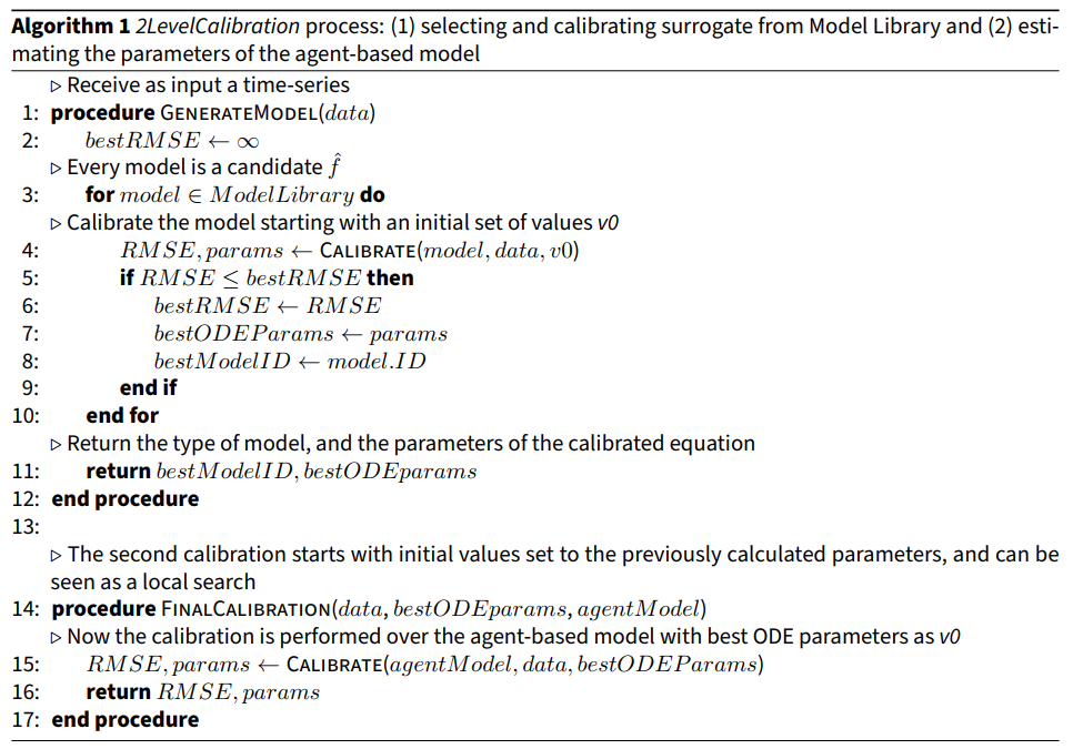
Algorithm 1 describes the whole process. The requirement of efficiency is fulfilled by the usage of the Model Library, which provides a lightweight method for the creation of the surrogate model. Note that we adopted RMSE to measure the error between observed data and the template curves in our Model Library, but it is possible to choose any preferred measure (e.g., MAPE, MSE etc) as long as the algorithm can properly differentiate between the modes of behaviour. Sometimes, such identification of the template curve can be done even visually, and the step of automatically selecting the template curve can be skipped and the user might go straight to the step of calibrating the surrogate model parameters.
With our method 2LevelCalibration we are able to combine several advantages of the previously mentioned techniques, without compromising the computational cost. As in Importance Sampling, we can concentrate on the hot spots of the search space. With the first step of our method (procedure GenerateModel from Algorithm 1), we mostly calibrate the parameters with samples that come from the cheapest model (the surrogate), just like in Multi Level Monte Carlo. As in History matching, the tested set of parameters is confronted against all historical system behaviour to increase our certainty on their values, although as we already have the structure of the behaviour pre-defined by our Model Library, this process is computationally cheaper and more precise. The use of the models from SD substitutes the step of sensitive analysis methods as the behavioural pattern of the system over time acts similarly as an indicator of the dominant parameters - in a sense, it acts as the stepwise regression. Similarly, as in Variance-based sensitivity analysis, we use the ODE’s parameters as a cluster of correlated parameters of the agent-based model, avoiding the Curse of Dimensionality. In the same way as ANOVA, we first analyse a group of parameters and then expand gradually the dimensionality of the analysis in the second step of 2LevelCalibration (procedure FinalCalibration from Algorithm 1).
Model library
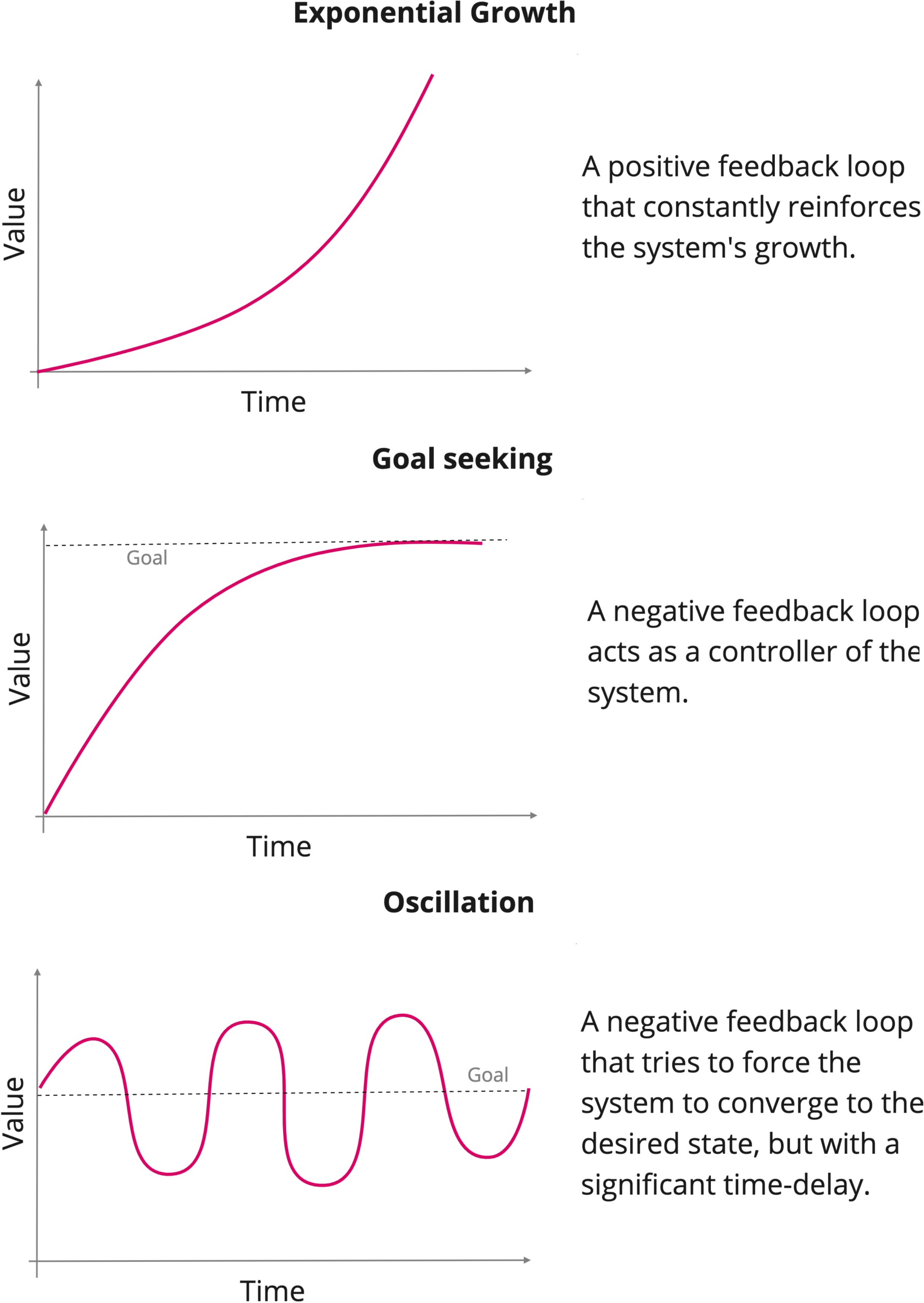
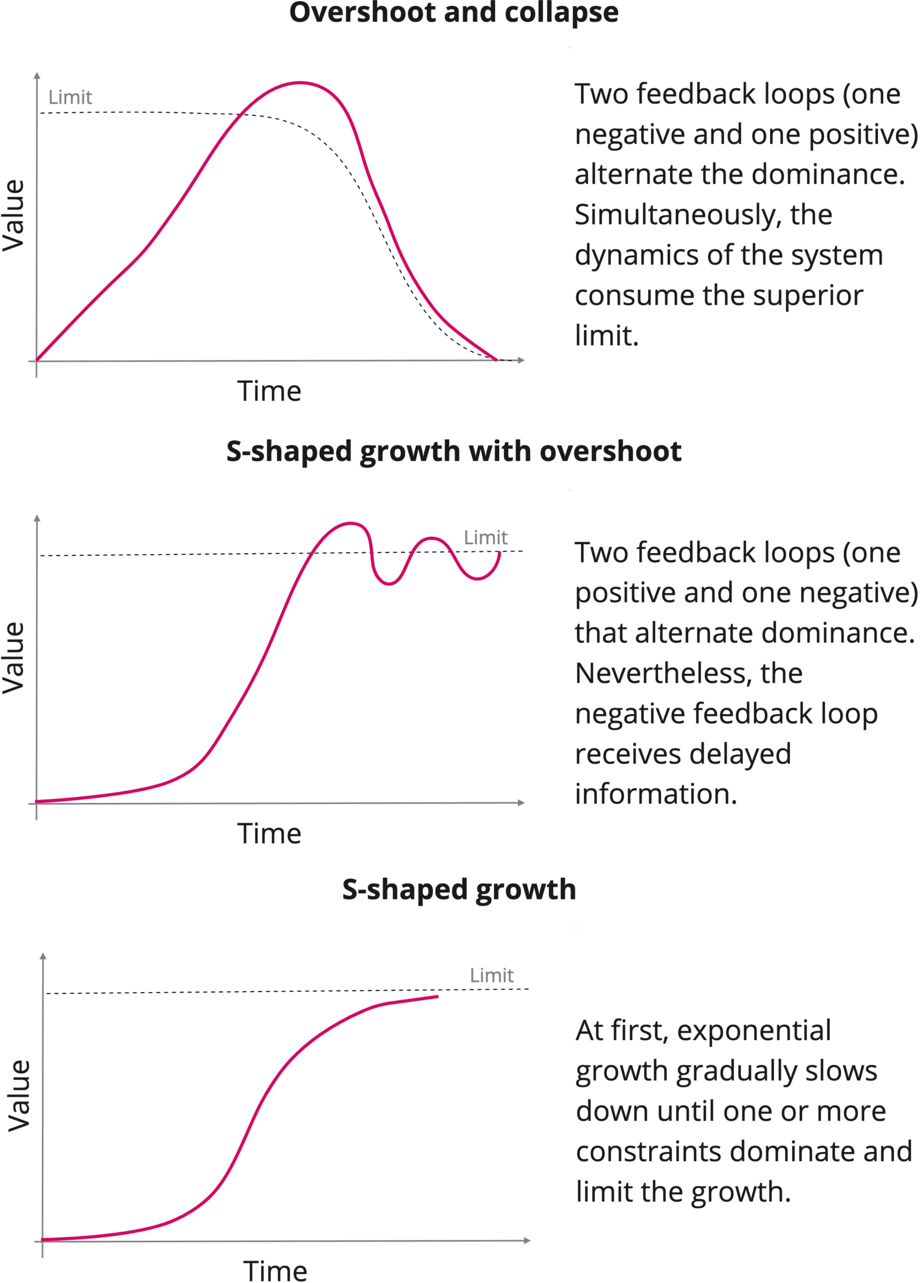
The first challenge of our method is to define the strategy to choose the function \(\hat{f}\) that describes the surrogate model in an inexpensive way. Thereafter, we propose to use a Model Library that incorporates the most common patterns of behaviours in social systems. Our decision is based on the fact that in SD there are some canonical behaviours, known as fundamental modes (Sterman 2000), whose originating structures are identified and presented in Figure 3.
When the basic modes of behaviour25 are combined and interact with each other in a nonlinear manner, other more complex behavioural pattern emerge (Sterman 2000). Still, they are recurrent both on physical and social systems and are presented in Figure 4. Other more complex behavioural modes were not implemented as their erratic behaviour makes their forecasts less useful and consequently limits the relevance of a parameter calibration task.
In our approach, collected data is compared against such template curves in the Model Library to infer which one better suits the observed phenomena, as represented in lines 3-10 in Algorithm 1.
The method used to calibrate both ODEs and agent-based model’s parameters is another cornerstone of our method, but it can be chosen freely as the effectiveness of our method stems from the multi-phase approach26. In order to demonstrate that a phased strategy satisfies our requirements for effectiveness and consistency, we executed an experiment comparing our 2LevelCalibration method coupled with different sampling techniques against the strategy of calibrating all the parameters at once of the agent-based model.
Housing market: A testbed for our approach
An iconic example of the strength of agent-based models was largely advocated after the housing market crisis in 2008. Several researchers have discussed the adequacy of agent-based models in foreseeing the economic crisis, such as in Farmer & Foley (2009) and in The Economist (2010).
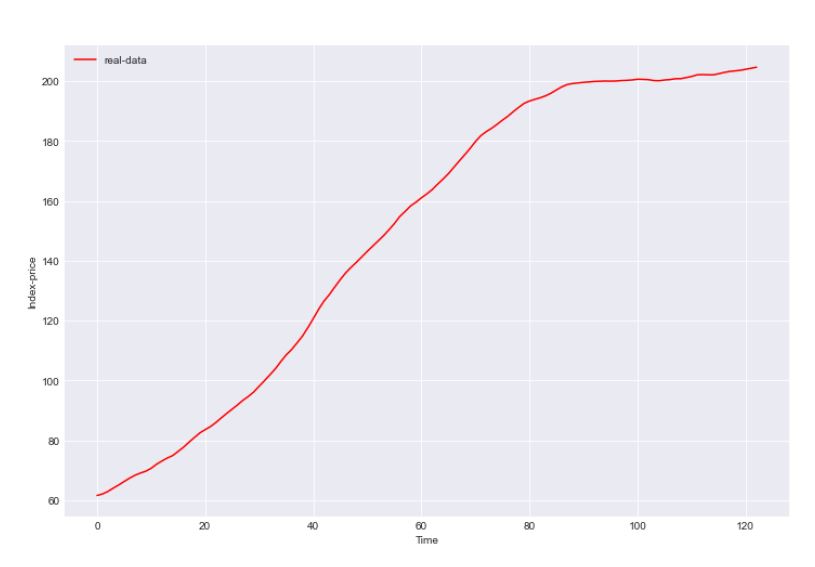
The housing market in São Paulo was chosen for our experiment. Data was obtained from a publicly available repository FIPEZAP (FIPE 2023). For this experiment, we will consider a time series of the price of \(m^2\) in São Paulo, the biggest city in Brazil, from January 2008 to March 2018.
It is worth mentioning that we developed a model of the housing market to use as a testbed for the evaluation of the performance of our method and, above all, to validate whether it met our efficiency and consistency requirements. The model presented here is not meant to describe the housing market in the best possible way - the model should simply contain a level of complexity that portrays a common agent-based model under development to test our calibration method and to show how the process of downscaling the parameters of the ODE can be aided by the use of structure feedback loops diagrams from SD. Moreover, with a testbed model, we were able to add certain properties that are the major causes of parameter calibration methods’ non-convergence, which are notably a large number of dependent parameters and those that follow probability distributions that might present infinite variance.
It is straightforward that the dynamics of prices of the housing market emerge from the interaction of buyers and sellers. Buyers clearly have a higher limit of money they can afford to pay for a house (this limit could stem from income and credit access) that is described in our model as savings variable, which cannot be exceeded under any circumstance. Having available a given amount of money does not mean that this will be the offered price for the house, though. A buyer will analyse the charged prices in the near past to see what was the average practiced price for a target region. This concept is represented in the model as variable proposedPrice, that is calculated in a way that savings is not surpassed and allowing a slight increase on current practiced prices by a percentage that is individual, and that describes the behavioural economic concept of willingness to pay, modelled as wtp.
Seller agents, on the other hand, try to increase houses’ prices without a higher superior constraint, but they have a lower value they accept for an offer, as values below this limit are credited to be less than the house is worth (variable lowerPrice). This lower price cannot diverge too much from the practiced price in the near past and is also influenced by the time the seller is offering his house without a buyer - the longer the time the seller does not succeed in selling the house, the lower the price he accepts as an offer. Additionally, how much a seller waits until he decreases the price is also particular to each agent and is incorporated in our model as variable noSell. How much he decreases the charged price and the lowest price is individual and is modelled as variable profitMargin. Otherwise, if a sell was successful, the seller increases the asked price and the lowest price for the next timestep - both variables are updated according to the individual profitMargin variable.
In a nutshell, the execution of the model’s simulation requires the calibration of those variables:
- price0, that reflects the price used as a starting reference of practiced price. This variable should be calibrated and not only inferred as the initial value of the time series: the optimum combination of parameters might not contain exactly this value.
- savings, which determine the maximum amount of money a buyer can afford to pay. Each buyer presents its own savings, that is set at the moment of its creation. The calibration process should determine an average value for the savings variable, that will be used as the mean of a student’s T distribution with 3 degrees of freedom, and from where the individual value of a buyer’s savings should be sampled from. The probability distribution was chosen in a way to generate savings values with large variance, testing the performance of the calibration method under conditions that are frequent under social systems and that at the same time make most traditional methods fail.
- wtp, that describes how much a buyer accepts to inflate the current practiced prices in order to purchase the house. Variable wtp represents the percentage the agent uses to inflate practiced prices in order to calculate proposedPrice. The calibration method should estimate the value of the mean of a normal distribution from which the simulator samples to determine the individual value for the buyer during its creation process.
- profitMargin variable determines the percentage by which the seller will inflate current practiced prices when calculating the price to charge for his house. Again, profitMargin values’ are particular for each seller and are within the interval of 0 and 1. The parameter calibration method stipulates the mean of a normal distribution that dictates the distribution of profitMargin values for the population of seller agents.
- lowerPrice represents the bottom price a seller is willing to accept as an offer for this house. Clearly, lowerPrice should be inferior to askedPrice, that is the result of applying agent’s personal profitMargin to the current price. In our model, lowerPrice is defined also as a percentage, varying from 0 to 1, which is applied over profitMargin multiplied by askedPrice.
- noSell describes how many timesteps the seller waits until he decreases the askedPrice. This variable’s range is defined by the interval between 1 and the maximum value provided by the calibration method. Each seller has a uniform probability of receiving one of the values within this interval.
This model was used in a way that two types of agents (50 sellers and 50 buyers) repeatedly negotiate houses’ prices. To calibrate the parameters of the model, we should find the set of parameters that generates a time series that depicts more closely the evolution of real-world prices. The source code of the simulation can be found at https://github.com/priavegliano/2LevelCalibration.
Constructing the surrogate model with System Dynamics
As we can see in Figure 5, the evolution of prices over time resembles the S-shaped growth fundamental mode. Mathematically, the S-shaped growth pattern can be modelled as the following ordinary differential equation (ODE), which was used as the surrogate function \(\hat{f}\) in our experiment:
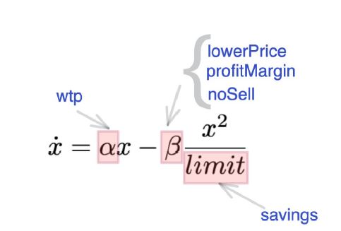
| \[ \frac{d \hat{f}}{dt} = \dot{x} = \alpha x - \beta \frac{x^2}{limit}\] | \[(1)\] |
In this context, variable \(x\) represents the index price portrayed by the time series. We can see that there are two acting forces that define how much \(x\) vary from one time step to another, that are precisely the positive feedback loop, present on the therm \(\alpha x\) of the equation, and the balancing negative loop, represented by \(\beta \frac{x^2}{limit}\).
From the dynamics of the S-shaped growth pattern of feedback dominance, we can relate the \(\alpha\) variable that governs the positive feedback loop to the forcing power of buyers, which increases the practiced prices with their associated wtp variable. On the other hand they simultaneously contribute to limiting this increase with their associated variable savings, which can be represented by variable limit of the function \(\hat{f}\). Sellers, on the other hand, also interfere on the negative feedback loop by determining the lowerPrice that they accept. As the definition of the lowerPrice is dependent of variables profitMargin and noSell, we have encapsulated all of these variables into \(\beta\) term of \(\hat{f}\). The reaction between parameters of surrogate function \(\hat{f}\) and the parameters of the agent-based model is depicted in Figure 6. Notably, that is a benefit brought by the usage of SD’s fundamental modes of behaviour: by bringing along a structure of positive and negative feedback loops that result in the observed behaviour, it is easier to perform the downscale of the parameters (i.e, it is easier to identify which of the parameters of the agent-based models are represented on the reduced set of parameters of the surrogate model).
Experiment
In the experiment, our method 2LevelCalibration was applied in the following way: the first step was to select the method to calibrate the parameters of the surrogate models in our Model Library to automatically identify the surrogate function \(\hat{f}\) that best describes the observed output of the system. After performing this step, we receive calibrated values for variables \(\alpha\), \(\beta\), limit and price0 (i.e., we have calibrated the parameters of our surrogate function \(\hat{f}\)). We then used these calibrated variables as the initial values for the process of calibration of the six parameters that describe the behaviour of our complete agent-based model. With this approach, we were able to find more easily potential areas of a good combination of parameters. In our experiment, we applied the same calibration method used to estimate the parameters of the surrogate function (4 variables) and the full agent-based models (6 parameters), but this is not a constraint of our approach, as we could apply different calibration methods on the different stages.
In order to comparatively assess the performance of our method, we used the outcome of calibrating the agent-based model directly as a benchmark, without using the surrogate, which we will reference henceforth as raw calibration.
As the model exhibits randomness, we have executed the calibration process, both with our proposed method and with the raw calibration, 130 times. Moreover, to account whether the performance was actually associated with the process of performing a multi-stage calibration, and not with the selected method for parameter calibration, we compared the outcome of two different calibration methods: CMA-ES and Monte Carlo Markov Chain. Both methods were selected because they are agnostic to some important properties of social agent-based models. The results of both calibration processes are shown in Table 2.
| MCMC | CMA-ES | |||
| Mean | \(\sigma\) | Mean | \(\sigma\) | |
| Raw calibration | 28.86 | 16.24 | 16.81 | 10.07 |
| 2LevelCalibration | 20.35 | 9.36 | 9.77 | 1.13 |
In most executions, the raw calibration was not able to find suitable parameters to satisfactory replicate important features of the real system, shown by higher mean error of the model with the raw calibration. This is quite relevant as this can be a misleading result: this could invalidate a viable agent-based model that did not capture the dynamics of real-world due to poor parameter calibration. On the other hand, we can clearly see that using our 2LevelCalibration method we can obtain a reasonably good result generated by the simulation (smaller error) in a consistent manner (smaller deviation). This is an important feature, as parameter calibration can make part of the modelling process of agent-based simulation. Reaching quickly the desired behaviour can enhance this process, as one can easily see if the definitions and assumptions of the model are correct. Moreover, our method is flexible enough to be used in combination with other approaches, such as in History matching, by preventing the discard of useful portions of the search space.
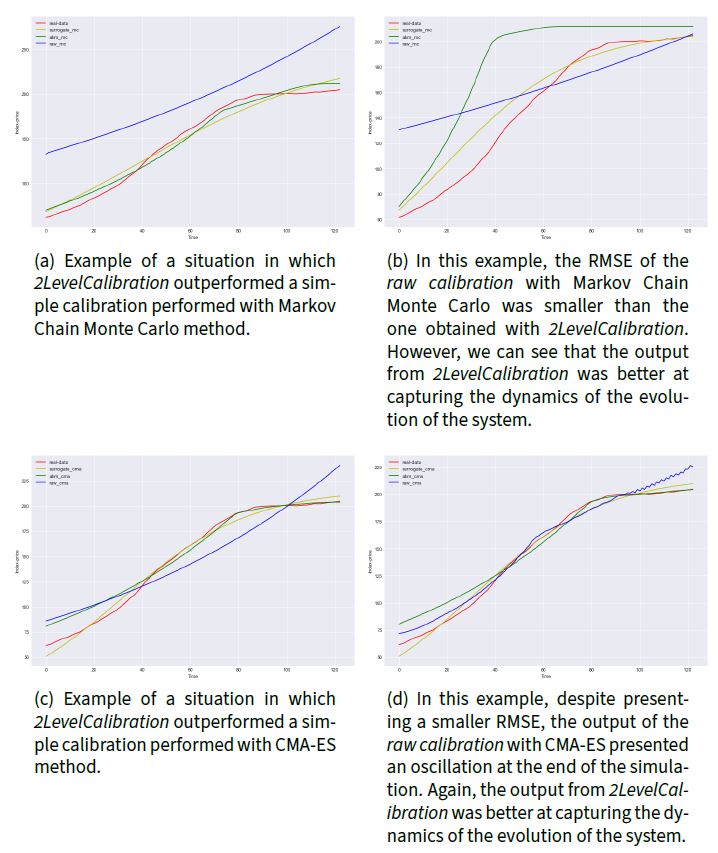
Figure 7 depicts comparatively several outputs of different calibration strategies. In some situations, we can see that even when RMSE indicated a superiority in performance of raw calibration, the output of 2LevelCalibration was better at emulating the dynamic of real-world data (the shape of the simulator output was similar to the shape of real data despite a larger total distance point to point). In order to overcome this limitation of RMSE analysis, the Fréchet distance was also applied to assess how much the output of the calibrated agent-based simulator properly captured the dynamics of real-world data (Har-Peled & others 2002). The Fréchet distance is a widely adopted measure (Aronov et al. 2006) that was chosen to capture how similar the behaviour of curves is over time: as it has embedded on its calculation the structure of the target curves (Har-Peled & Raichel 2014), Fréchet distance measures if both curves go simultaneously in the same direction. The comparative performance of the Raw calibration and our 2LevelCalibration is presented in Table 3.
| MCMC | CMA-ES | |||
| Mean | \(\sigma\) | Mean | \(\sigma\) | |
| Raw calibration | 38.55 | 25.26 | 35.57 | 18.24 |
| 2LevelCalibration | 25.87 | 16.20 | 19.01 | 1.50 |
Given the randomness of the model and the calibration methods, we can see that sometimes the raw calibration provides good results. This is not a guaranteed behaviour though, as often the output of the calibrated model differs markedly from real-world data. On the other hand, our method provides satisfactory and consistent results, converging to the desired behaviour. This occurs because generating the surrogate model and performing a calibration on a reduced space search eases the task of finding suitable values. It is known that the higher the dimension of the search space, the harder it is to find the zone of interest (Tarantola 2005). The step of defining the surrogate model provided clues about the region of interest to perform the search for suitable values, assuring the consistency of the results.
Conclusion
We have proposed a new method of parameter calibration for social agent-based models. Our contribution is twofold: firstly and most importantly, is the use of a surrogate model to reduce space search dimensionality, assuring the convergence of the result; secondly, we have presented an efficient method to identify the surrogate model, based on a Model Library that wisely explores SD’s fundamental modes of behaviour. We validated both concepts with real-world data from the housing market scenario, comparing the performance of our method against two robust and agnostic methods for parameter calibration.
Our 2LevelCalibration strategy showed valuable properties for the parameter calibration task. It has a lightweight implementation that performs a cheap model order reduction step because it relies on a few predefined patterns of behaviour from our Model Library. Additionally, it achieves consistent results with lower uncertainty, denoted by the substantial reduction of the mean error and, more importantly, its associated standard deviation. With these two important properties, our method 2LevelCalibration emerges as an option for the recurrent and challenging task of parameter calibration of agent-based models as long as the dynamics of the target system can be modelled with an analytical set of differential equations.
Notes
The mean and variance of a finite set of sample is, of course, finite, but the probability distribution that gives rise to the observed samples might present infinite mean or variance, depending on its parameters.↩︎
It is common to find an allusion to 2k Factorial or 3k Factorial in the literature, especially in DoE-related works. This denomination tells us in how many different levels we have divided the range of variation of our target variable. For instance, a 2k Factorial design splits the possible values between high and low. It is advisable to start the experiments with a smaller number of levels to identify major interactions and contributions of each parameter, sparing also computational resources (Cox & Reid 2000).↩︎
When one of the involved variables belong to a heavy-tailed family of probability distributions, the number of samples to properly calculate the mean and variance can be prohibitive (Taleb 2020).↩︎
When Sobol’ indices are calculated for black-box models and cannot be based on the analytical formula (Brevault et al. 2013).↩︎
This situation can be overcome with the construction of surrogate models (Hart et al. 2017).↩︎
These terms are used interchangeably in this work.↩︎
The complexity of a Gaussian Process is cubic (Liu et al. 2020) and thus it can be prohibitive depending on the number of variables involved.↩︎
Random variables that belong to the Power Law class of probability distributions can present infinite moments. The famous 80-20 Pareto distribution, for instance, presents an infinite variance.↩︎
Those samples, in reality, bring much more information than any regular sample.↩︎
An adapted version of the quasi-random sampling based on Sobol’ sequences↩︎
More precisely, extremely boosted gradient trees (XG-Boost)↩︎
Deep Learning Neural Net↩︎
Nearly Orthogonal version↩︎
The method requires that at least one sample is classified into a desired category↩︎
CatBoost, a decision tree boosting algorithm↩︎
Particle filtering, that is based on importance sampling↩︎
Support vector regression↩︎
Based on Random Forest↩︎
ROPE: Robust Optimized Parameter Estimation, a regression with steroids (Bárdossy & Singh 2008)↩︎
Coupled with Bayesian Optimization↩︎
Adam optimizer, that relies on the first-order derivative and fast convergence↩︎
With an emphasis on a simulation pipeline from data to results exploration, that encompasses model parameter calibration. The focus of the framework though is agent-based models for demography, more restrictive than the broad use of agent-based models in general.↩︎
By agnostic we refer to methods that are capable of properly approximating a broad range of models with different properties.↩︎
Consistency is especially desired on an agent-based modelling approach, as a model structure can be completely disregarded if results are not satisfactory; but the error could be on the parameters that were not properly calibrated, not the model structure itself.↩︎
Every mode of behaviour is described as one model in our Library.↩︎
In fact, one could choose different sampling strategies: one for calibrating ODEs parameters and one for the agent-based models.↩︎
References
ARONOV, B., Har-Peled, S., Knauer, C., Wang, Y., & Wenk, C. (2006). Fréchet distance for curves, revisited. European symposium on algorithms. [doi:10.1007/11841036_8]
BANKS, D. L., & Hooten, M. B. (2021). Statistical challenges in agent-based modeling. The American Statistician, 75(3), 235–242. [doi:10.1080/00031305.2021.1900914]
BARDE, S., & van der Hoog, S. (2017). An empirical validation protocol for large-scale agent-based models. Bielefeld Working Papers in Economics and Management. Available at: https://papers.ssrn.com/sol3/papers.cfm?abstract_id=2992473 [doi:10.2139/ssrn.2992473]
BARRON, A. R. (1993). Universal approximation bounds for superpositions of a sigmoidal function. IEEE Transactions on Information Theory, 39(3), 930–945. [doi:10.1109/18.256500]
BÁRDOSSY, A., & Singh, S. (2008). Robust estimation of hydrological model parameters. Hydrology and Earth System Sciences, 12(6), 1273–1283.
BIEGLER, L., Biros, G., Ghattas, O., Heinkenschloss, M., Keyes, D., Mallick, B., Marzouk, Y., Tenorio, L., van Bloemen Waanders, B., & Willcox, K. (2011). Large-Scale Inverse Problems and Quantification of Uncertainty. Hoboken, NJ: John Wiley & Sons.
BIJAK, J. (2022). Towards Bayesian Model-Based Demography: Agency, Complexity and Uncertainty in Migration Studies. Berlin Heidelberg: Springer. [doi:10.1007/978-3-030-83039-7_2]
BREVAULT, L., Balesdent, M., Bérend, N., & Le Riche, R. (2013). Comparison of different global sensitivity analysis methods for aerospace vehicle optimal design. 10th World Congress on Structural and Multidisciplinary Optimization, WCSMO-10. [doi:10.2514/1.j054121]
BROOKS, S., Gelman, A., Jones, G., & Meng, X.-L. (2011). Handbook of Markov Chain Monte Carlo. Boca Raton, FL: CRC Press.
CARRELLA, E. (2021). No free lunch when estimating simulation parameters. Journal of Artificial Societies and Social Simulation, 24(2), 7. [doi:10.18564/jasss.4572]
CHANDRASHEKAR, G., & Sahin, F. (2014). A survey on feature selection methods. Computers & Electrical Engineering, 40(1), 16–28. [doi:10.1016/j.compeleceng.2013.11.024]
CHEN, X., Liu, S., Sun, R., & Hong, M. (2018). On the convergence of a class of Adam-type algorithms for nonconvex optimization. arXiv preprint. arXiv:1808.02941
CHEN, Y., Embrechts, P., & Wang, R. (2022). An unexpected stochastic dominance: Pareto distributions, catastrophes, and risk exchange. arXiv preprint. arXiv:2208.08471
CIRILLO, P., & Taleb, N. N. (2016). On the statistical properties and tail risk of violent conflicts. Physica A: Statistical Mechanics and Its Applications, 452, 29–45. [doi:10.1016/j.physa.2016.01.050]
CIRILLO, P., & Taleb, N. N. (2020). Tail risk of contagious diseases. Nature Physics, 16(6), 606–613. [doi:10.1038/s41567-020-0921-x]
CONTI, S., Gosling, J. P., Oakley, J. E., & O’Hagan, A. (2009). Gaussian process emulation of dynamic computer codes. Biometrika, 96(3), 663–676. [doi:10.1093/biomet/asp028]
COX, D. R., & Reid, N. (2000). The Theory of the Design of Experiments. Boca Raton, FL: Chapman and Hall - CRC.
DILAVER, Ö., & Gilbert, N. (2023). Unpacking a black box: A conceptual anatomy framework for agent-Based social simulation models. Journal of Artificial Societies and Social Simulation, 26(1), 4. [doi:10.18564/jasss.4998]
EBDEN, M. (2015). Gaussian processes: A quick introduction. arXiv preprint. arXiv:1505.02965
FAGIOLO, G., Guerini, M., Lamperti, F., Moneta, A., & Roventini, A. (2019). Validation of agent-based models in economics and finance. In C. Beisbart & N. J. Saam (Eds.), Computer Simulation Validation (pp. 763–787). Berlin Heidelberg: Springer. [doi:10.1007/978-3-319-70766-2_31]
FARMER, J. D., & Foley, D. (2009). The economy needs agent-based modelling. Nature, 460(7256), 685–686. [doi:10.1038/460685a]
FEDOTENKOV, I. (2020). A review of more than one hundred Pareto-tail index estimators. Statistica, 80(3), 245–299.
FIPE. (2023). BIndice FIPEZAP. Available at: https://www.fipe.org.br/pt-br/indices/fipezap
FONOBEROVA, M., Fonoberov, V. A., & Mezić, I. (2013). Global sensitivity/uncertainty analysis for agent-based models. Reliability Engineering & System Safety, 118, 8–17. [doi:10.1016/j.ress.2013.04.004]
FORRESTER, J. W. (1994). System dynamics, systems thinking, and soft OR. System Dynamics Review, 10(2-3), 245–256. [doi:10.1002/sdr.4260100211]
FRANGOS, M., Marzouk, Y., Willcox, K., & van Bloemen Waanders, B. (2010). Surrogate and Reduced-Order Modeling: A Comparison of Approaches for Large-Scale Statistical Inverse Problems. Hoboken, NJ: John Wiley & Sons. [doi:10.1002/9780470685853.ch7]
FRAZIER, P. I. (2018). A tutorial on Bayesian optimization. arXiv preprint. arXiv:1807.02811
GAN, Y., Duan, Q., Gong, W., Tong, C., Sun, Y., Chu, W., Ye, A., Miao, C., & Di, Z. (2014). A comprehensive evaluation of various sensitivity analysis methods: A case study with a hydrological model. Environmental Modelling & Software, 51, 269–285. [doi:10.1016/j.envsoft.2013.09.031]
GARG, A., Yuen, S., Seekhao, N., Yu, G., Karwowski, J. A., Powell, M., Sakata, J. T., Mongeau, L., JaJa, J., & Li-Jessen, N. Y. (2019). Towards a physiological scale of vocal fold agent-based models of surgical injury and repair: Sensitivity analysis, calibration and verification. Applied Sciences, 9(15), 2974. [doi:10.3390/app9152974]
GELMAN, A. (2005). Analysis of variance—why it is more important than ever. The Annals of Statistics, 33(1), 1–53. [doi:10.1214/009053604000001048]
GEYER, C. J. (1991). Markov chain Monte Carlo maximum likelihood. Available at: https://conservancy.umn.edu/handle/11299/58440
GILBERT, N. (2002). Varieties of emergence. Social Agents: Ecology, Exchange and Evolution, 41–50.
GRANGER, C. W. (1968). Some aspects of the random walk model of stock market prices. International Economic Review, 9(2), 253–257. [doi:10.2307/2525478]
GRAZZINI, J., Richiardi, M. G., & Tsionas, M. (2017). Bayesian estimation of agent-based models. Journal of Economic Dynamics and Control, 77, 26–47. [doi:10.1016/j.jedc.2017.01.014]
GRIMM, V., & Berger, U. (2016). Robustness analysis: Deconstructing computational models for ecological theory and applications. Ecological Modelling, 326, 162–167. [doi:10.1016/j.ecolmodel.2015.07.018]
GRIMM, V., Revilla, E., Berger, U., Jeltsch, F., Mooij, W. M., Railsback, S. F., Thulke, H.-H., Weiner, J., Wiegand, T., & DeAngelis, D. L. (2005). Pattern-oriented modeling of agent-based complex systems: Lessons from ecology. Science, 310(5750), 987–991. [doi:10.1126/science.1116681]
HAMILL, L., & Gilbert, N. (2015). Agent-Based Modelling in Economics. Hoboken, NJ: John Wiley & Sons.
HANSEN, N. (2006). The CMA evolution strategy: A comparing review. In J. A. Lozano, P. Larrañaga, I. Inza, & E. Bengoetxea (Eds.), Towards a New Evolutionary Computation (pp. 75–102). Springer. [doi:10.1007/3-540-32494-1_4]
HAR-PELED, S., & others. (2002). New similarity measures between polylines with applications to morphing and polygon sweeping. Discrete & Computational Geometry, 28(4), 535–569.
HAR-PELED, S., & Raichel, B. (2014). The fréchet distance revisited and extended. ACM Transactions on Algorithms (TALG), 10(1), 1–22. [doi:10.1145/2532646]
HART, J. L., Alexanderian, A., & Gremaud, P. A. (2017). Efficient computation of Sobol’ indices for stochastic models. SIAM Journal on Scientific Computing, 39(4), 1514–1530. [doi:10.1137/16m106193x]
HENSMAN, P., & Masko, D. (2015). The impact of imbalanced training data for convolutional neural networks. Degree Project in Computer Science, KTH Royal Institute of Technology
HUNTER, E., Mac Namee, B., & Kelleher, J. D. (2017). A taxonomy for agent-based models in human infectious disease epidemiology. Journal of Artificial Societies and Social Simulation, 20(3), 2. [doi:10.18564/jasss.3414]
JASRA, A., Law, K., & Suciu, C. (2020). Advanced multilevel Monte Carlo methods. International Statistical Review, 88(3), 548–579. [doi:10.1111/insr.12365]
JOLLIFFE, I. T., & Cadima, J. (2016). Principal component analysis: A review and recent developments. Philosophical Transactions of the Royal Society A: Mathematical, Physical and Engineering Sciences, 374(2065), 20150202. [doi:10.1098/rsta.2015.0202]
KENNEDY, M. C., & O’Hagan, A. (2001). Bayesian calibration of computer models. Journal of the Royal Statistical Society: Series B (Statistical Methodology), 63(3), 425–464. [doi:10.1111/1467-9868.00294]
KINAL, T., & Lahiri, K. (1983). Specification error analysis with stochastic regressors. Econometrica, 51(4), 1209–1219. [doi:10.2307/1912059]
KINGMA, D. P., & Ba, J. (2014). Adam: A method for stochastic optimization. arXiv preprint. arXiv:1412.6980
KOTTHOFF, F., & Hamacher, T. (2022). Calibrating agent-Based models of innovation diffusion with gradients. Journal of Artificial Societies and Social Simulation, 25(3), 4. [doi:10.18564/jasss.4861]
KUCHERENKO, S., Albrecht, D., & Saltelli, A. (2015). Exploring multi-dimensional spaces: A comparison of Latin hypercube and quasi Monte Carlo sampling techniques. arXiv preprint. Available at: https://arxiv.org/abs/1505.02350.
LAMAMRA, K., Vaidyanathan, S., Azar, A. T., & Salah, C. B. (2017). Chaotic system modelling using a neural network with optimized structure. In A. T. Azar, S. Vaidyanathan, & A. Ouannas (Eds.), Fractional Order Control and Synchronization of Chaotic Systems (pp. 833–856). Berlin Heidelberg: Springer. [doi:10.1007/978-3-319-50249-6_29]
LAMBONI, M., Iooss, B., Popelin, A.-L., & Gamboa, F. (2013). Derivative-based global sensitivity measures: General links with Sobol’ indices and numerical tests. Mathematics and Computers in Simulation, 87, 45–54. [doi:10.1016/j.matcom.2013.02.002]
LAMPERTI, F., Roventini, A., & Sani, A. (2018). Agent-based model calibration using machine learning surrogates. Journal of Economic Dynamics and Control, 90, 366–389. [doi:10.1016/j.jedc.2018.03.011]
LIU, H., Ong, Y.-S., Shen, X., & Cai, J. (2020). When Gaussian process meets big data: A review of scalable GPs. IEEE Transactions on Neural Networks and Learning Systems, 31(11), 4405–4423. [doi:10.1109/tnnls.2019.2957109]
LIU, Z., Rexachs, D., Epelde, F., & Luque, E. (2017). A simulation and optimization based method for calibrating agent-based emergency department models under data scarcity. Computers & Industrial Engineering, 103, 300–309. [doi:10.1016/j.cie.2016.11.036]
LORSCHEID, I., Heine, B.-O., & Meyer, M. (2012). Opening the “black box” of simulations: Increased transparency and effective communication through the systematic design of experiments. Computational and Mathematical Organization Theory, 18(1), 22–62. [doi:10.1007/s10588-011-9097-3]
LU, J. (2022). Gradient descent, stochastic optimization, and other tales. arXiv preprint. arXiv:2205.00832
LUX, T. (2018). Estimation of agent-based models using sequential Monte Carlo methods. Journal of Economic Dynamics and Control, 91, 391–408. [doi:10.1016/j.jedc.2018.01.021]
MANDELBROT, B., & Taylor, H. M. (1967). On the distribution of stock price differences. Operations Research, 15(6), 1057–1062. [doi:10.1287/opre.15.6.1057]
MARSHALL, B. D., & Galea, S. (2015). Formalizing the role of agent-based modeling in causal inference and epidemiology. American Journal of Epidemiology, 181(2), 92–99. [doi:10.1093/aje/kwu274]
MAUHE, N., Izquierdo, L. R., & Izquierdo, S. S. (2023). Social simulation models as refuting machines. Journal of Artificial Societies and Social Simulation, 26(2), 8. [doi:10.18564/jasss.5076]
MCCULLOCH, J., Ge, J., Ward, J. A., Heppenstall, A., Polhill, J. G., & Malleson, N. (2022). Calibrating agent-Based models using uncertainty quantification methods. Journal of Artificial Societies and Social Simulation, 25(2), 1. [doi:10.18564/jasss.4791]
MENG, X., Li, Z., Zhang, D., & Karniadakis, G. E. (2020). PPINN: Parareal physics-informed neural network for time-dependent PDEs. Computer Methods in Applied Mechanics and Engineering, 370, 113250. [doi:10.1016/j.cma.2020.113250]
MORRIS, M. D. (1991). Factorial sampling plans for preliminary computational experiments. Technometrics, 33(2), 161–174. [doi:10.1080/00401706.1991.10484804]
MOSS, S. (2008). Alternative approaches to the empirical validation of agent-based models. Journal of Artificial Societies and Social Simulation, 11(1), 5.
MYERS, R. H., Montgomery, D. C., & Anderson-Cook, C. M. (2016). Response Surface Methodology: Process and Product Optimization Using Designed Experiments. Hoboken, NJ: John Wiley & Sons.
NAIR, J., Wierman, A., & Zwart, B. (2013). The fundamentals of heavy-tails: Properties, emergence, and identification. Proceedings of the ACM SIGMETRICS/International Conference on Measurement and Modeling of Computer Systems [doi:10.1145/2465529.2466587]
OAKLEY, J. E., & O’Hagan, A. (2004). Probabilistic sensitivity analysis of complex models: A Bayesian approach. Journal of the Royal Statistical Society: Series B (Statistical Methodology), 66(3), 751–769. [doi:10.1111/j.1467-9868.2004.05304.x]
OAKLEY, J., & O’Hagan, A. (2002). Bayesian inference for the uncertainty distribution of computer model outputs. Biometrika, 89(4), 769–784. [doi:10.1093/biomet/89.4.769]
OWEN, A., Dick, J., & Chen, S. (2014). Higher order Sobol’ indices. Information and Inference: A Journal of the IMA, 3(1), 59–81. [doi:10.1093/imaiai/iau001]
OWEN, A., & Zhou, Y. (2000). Safe and effective importance sampling. Journal of the American Statistical Association, 95(449), 135–143. [doi:10.1080/01621459.2000.10473909]
PAPADELIS, S., & Flamos, A. (2019). An application of calibration and uncertainty quantification techniques for agent-based models. In H. Doukas, A. Flamos, & J. Lieu (Eds.), Understanding Risks and Uncertainties in Energy and Climate Policy (p. 79). Berlin Heidelberg: Springer. [doi:10.1007/978-3-030-03152-7_3]
PAPADOPOULOS, S., & Azar, E. (2016). Integrating building performance simulation in agent-based modeling using regression surrogate models: A novel human-in-the-loop energy modeling approach. Energy and Buildings, 128, 214–223. [doi:10.1016/j.enbuild.2016.06.079]
RATTO, M., & Saltelli, A. (2002). An efficient approach to deal with the curse of dimensionality in sensitivity analysis computations. International Conference on Computational Science. [doi:10.1007/3-540-46043-8_19]
REDDI, S. J., Kale, S., & Kumar, S. (2019). On the convergence of Adam and beyond. arXiv preprint. arXiv:1904.09237
REINHARDT, O., Hilton, J., Warnke, T., Bijak, J., & Uhrmacher, A. M. (2018). Streamlining simulation experiments with agent-based models in demography. Journal of Artificial Societies and Social Simulation, 21(3), 9. [doi:10.18564/jasss.3784]
REUSSER, D. E., Buytaert, W., & Zehe, E. (2011). Temporal dynamics of model parameter sensitivity for computationally expensive models with the Fourier amplitude sensitivity test. Water Resources Research, 47(7). [doi:10.1029/2010wr009947]
ROBERTS, G. O., & Smith, A. F. (1994). Simple conditions for the convergence of the Gibbs sampler and Metropolis-Hastings algorithms. Stochastic Processes and Their Applications, 49(2), 207–216. [doi:10.1016/0304-4149(94)90134-1]
ROBINSON, S. (2008). Conceptual modelling for simulation Part I: Definition and requirements. Journal of the Operational Research Society, 59(3), 278–290. [doi:10.1057/palgrave.jors.2602368]
RUDER, S. (2016). An overview of gradient descent optimization algorithms. arXiv preprint. arXiv:1609.04747
SAKA, M., Hasançebi, O., & Geem, Z. (2016). Metaheuristics in structural optimization and discussions on harmony search algorithm. Swarm and Evolutionary Computation, 28, 88–97. [doi:10.1016/j.swevo.2016.01.005]
SALTELLI, A., & Bolado, R. (1998). An alternative way to compute fourier amplitude sensitivity test (FAST). Computational Statistics & Data Analysis, 26(4), 445–460. [doi:10.1016/s0167-9473(97)00043-1]
SALTELLI, A., Tarantola, S., & Chan, K.-S. (1999). A quantitative model-independent method for global sensitivity analysis of model output. Technometrics, 41(1), 39–56. [doi:10.1080/00401706.1999.10485594]
SCHÄFER, A. M., & Zimmermann, H. G. (2006). Recurrent neural networks are universal approximators. International Conference on Artificial Neural Networks
SHIELDS, M. D., Teferra, K., Hapij, A., & Daddazio, R. P. (2015). Refined stratified sampling for efficient Monte Carlo based uncertainty quantification. Reliability Engineering & System Safety, 142, 310–325. [doi:10.1016/j.ress.2015.05.023]
SIEGENFELD, A. F., & Bar-Yam, Y. (2020). An introduction to complex systems science and its applications. Complexity, 2020, 6105872. [doi:10.1155/2020/6105872]
SMITH, G. (2018). Step away from stepwise. Journal of Big Data, 5(1), 1–12.
SOBOL, I. M. (1990). Quasi-monte carlo methods. Progress in Nuclear Energy, 24(1-3), 55–61.
SPEED, T. (1987). What is an analysis of variance? The Annals of Statistics, 15(3), 885–910.
STERMAN, J. D. (2000). Business Dynamics - Systems Thinking and Modeling for a Complex World. New York, NY: McGraw-Hill.
SULLIVAN, T. J. (2015). Introduction to Uncertainty Quantification. Berlin Heidelberg: Springer.
TALEB, N. N. (2020). Statistical consequences of fat tails: Real world preasymptotics, epistemology, and applications. arXiv preprint. arXiv:2001.10488
TARANTOLA, A. (2005). Inverse Problem Theory and Methods for Model Parameter Estimation. SIAM. [doi:10.1137/1.9780898717921]
TESFATSION, L., & Judd, K. L. (2006). Handbook of Computational Economics: Agent-Based Computational Economics. Amsterdam: Elsevier.
THE Economist. (2010). Agents of change. Available at: https://www.economist.com/finance-and-economics/2010/07/22/agents-of-change
THIELE, J. C., Kurth, W., & Grimm, V. (2014). Facilitating parameter estimation and sensitivity analysis of agent-based models: A cookbook using NetLogo and R. Journal of Artificial Societies and Social Simulation, 17(3), 11. [doi:10.18564/jasss.2503]
VAN der Hoog, S. (2019). Surrogate modelling in (and of) agent-based models: A prospectus. Computational Economics, 53(3), 1245–1263. [doi:10.1007/s10614-018-9802-0]
VAN Dyke Parunak, H., Savit, R., & Riolo, R. L. (1998). Agent-based modeling vs. equation-based modeling: A case study and users’ guide. International Workshop on Multi-Agent Systems and Agent-Based Simulation [doi:10.1007/10692956_2]
VENKATRAMANAN, S., Lewis, B., Chen, J., Higdon, D., Vullikanti, A., & Marathe, M. (2018). Using data-driven agent-based models for forecasting emerging infectious diseases. Epidemics, 22, 43–49. [doi:10.1016/j.epidem.2017.02.010]
VERMEULEN, P. (2018). How fat is the top tail of the wealth distribution? Review of Income and Wealth, 64(2), 357–387. [doi:10.1111/roiw.12279]
VERNON, I., Goldstein, M., & Bower, R. (2014). Galaxy formation: Bayesian history matching for the observable universe. Statistical Science, 29(1), 81–90. [doi:10.1214/12-sts412]
WILLIAMS, C. K., & Rasmussen, C. E. (2006). Gaussian Processes for Machine Learning. Cambridge, MA: MIT Press.
ZEIGLER, B. P., Muzy, A., & Kofman, E. (2018). Theory of Modeling and Simulation: Discrete Event & Iterative System Computational Foundations. New York, NY: Academic Press. [doi:10.1016/b978-0-12-813370-5.00012-2]
ZHANG, Y., Li, Z., & ZHANG, Y. (2020). Validation and calibration of an agent-based model: A surrogate approach. Discrete Dynamics in Nature and Society, 2020(6946370). [doi:10.1155/2020/6946370]