ReMoTe-S. Residential Mobility of Tenants in Switzerland: An Agent-Based Model

, ,
and
aLaboratory for Human-Environment Relations in Urban Systems (HERUS), Environmental Engineering Institute (IIE), School of Architecture, Civil and Environmental Engineering (ENAC), École Polytechnique Fédérale de Lausanne (EPFL), Lausanne, Switzerland; bEuropean Commission Joint Research Centre, Italy
Journal of Artificial
Societies and Social Simulation 25 (2) 4![]()
<https://www.jasss.org/25/2/4.html>
DOI: 10.18564/jasss.4752
Received: 03-May-2021 Accepted: 22-Feb-2022 Published: 31-Mar-2022
Abstract
Sustainable housing is a key priority for Switzerland. To provide both environmentally and socio-culturally sustainable housing, Swiss property owners need to navigate the complex and context-specific system that articulates the match between households’ preferences and the dwellings available to them—i.e., residential mobility. In response to this need, this paper outlines ReMoTe-S, an agent-based model of tenants’ residential mobility in Switzerland. The model design is based on empirical research conducted with the tenants of three multifamily housing providers. It accounts for the life course of dwellings and households, during which the latter attempt to maximise their satisfaction, which is calculated as the correspondence between their desired housing functions (e.g. a status symbol) and the functions of dwellings. To illustrate the model’s potential uses, we explore the sensitivity of its outputs to changes in dwellings’ and buildings’ qualitative and quantitative features by looking at two key indicators of housing sustainability: floor space per capita and vacancy rate. We firstly observe that a supply dominated by medium-to-large dwellings and the application of less strict occupancy rules can result in housing underoccupancy. Secondly, it emerges that certain combinations of housing features engender a lower vacancy rate inasmuch as they more successfully generate housing functions. We conclude that by enabling housing providers to explore the complex human-environment interactions of the housing system, ReMoTe-S can be used to inform a sustainable management of housing stock.Introduction
Accounting for approximately a fourth of \(CO_{2}\) emissions and total energy consumption in Switzerland (IEA 2018a, 2018b), housing plays a crucial role in the transition of urban systems towards sustainability (Binder et al. 2020). While measures to reduce the environmental footprint of the residential sector are urgently needed, housing supply must also be congruent with the cultural and social conventions of the present and future households (Chiu 2004; Prochorskaite et al. 2016). Providing sustainable housing therefore requires a holistic understanding of the complex interplay between households’ needs (i.e., demand) and their environment (i.e., supply; Lawrence 2009; Pagani et al. 2020). This interplay is made explicit in the relocation process, whereby households match their housing requirements to the dwellings available to them (Clark 2012). This process is commonly investigated as subject in itself, whereby micro-level data are collected and used for empirical analyses (Mulder 1996; Rérat 2020). However, dynamic models are needed to investigate macro-level outcomes of all household simultaneous choices over time (Benenson 2004; Mulder 1996).
Agent-based models (ABM) are particularly suitable for the exploration of real-world systems dynamics emerging from the interaction of agents and their individual preferences (Friege et al. 2016; Nikolic & Ghorbani 2011). Several theory-based and empirical ABMs of urban residential choice exist. However, despite their apparent comprehensiveness, these models are not applicable to all urban realms as cultural, political, economic and social contexts have a remarkable influence on residential settings and preferences (Booi & Boterman 2020; Lawrence & Barbey 2014).
In particular, Swiss housing differs markedly from housing in other OECD countries. In Switzerland, nearly two-thirds of the population are tenants whose rights are protected by a rent control legislation limiting landlords’ ability to raise rents and evict them at will (FSO 2017). A share of rental housing is populated by housing cooperatives, whose management of tenants differs from that of private landlords or asset managers. Furthermore, although housing quality and conditions are reported as being very satisfactory (Rabinovich 2009), finding a dwelling is not an easy endeavour considering the lower than ‘natural’ vacancy rate (2.7% in 2019) – in particular for the cities of Lausanne (0.4%) and Zurich (0.1%; Werczberger 1997; Wüest Partner 2020; Zimmermann 1992).
To provide housing that is both environmentally and socio-culturally sustainable, Swiss property owners need to navigate the above-described complexity—i.e., to account for the effects of households’ housing-related preferences and decisions as well as the tenure- and context-specific factors affecting them. In response to this need, this paper outlines ReMoTe-S, an agent-based model of residential mobility of tenants in Switzerland. The model is based on assumptions derived from empirical qualitative and quantitative research conducted with the tenants of three multifamily housing providers. Its goal is to foster a holistic understanding of the reciprocal influence between households and dwellings and thereby inform a sustainable management of the simulated housing stock.
This paper is organised as follows. Section 2 contextualises and illustrates the theoretical framework and assumptions underlying the model design. Section 3 introduces the ABM, including an overview of its agents, the model initialisation, and its sub-models. Section 4 concisely describes the model’s calibration and verification. Section 5 exemplifies potential model’s uses; it presents the setup and results of two ‘what-if’ experiments, where the concepts of housing environmental and socio-cultural sustainability are operationalised in quantitative and qualitative terms. More specifically, the first experiment consists in varying the size of the dwellings supplied to observe effects on average floor area per capita—a crucial indicator of resources and energy consumption in housing (Ellsworth-Krebs 2020; Karlen et al. 2021; Lorek & Spangenberg 2019; Pagani et al. 2020). The second experiment explores and compares the outcomes of the supply of dwellings with ‘sustainable’ qualitative features (e.g., closeness to public transports) and ‘unsustainable’ ones (e.g., parking places). Here, the average vacancy rate of dwellings in the model is used as an indicator to assess their correspondence with households’ preferences and needs (Haase et al. 2010). Finally, Section 6 discusses the theoretical contributions, validity, and limitations of ReMoTe-S. The paper concludes with recommendations for the three housing providers and future research pathways towards a sustainable management of their residential building stock.
Theoretical Framework and Previous Work
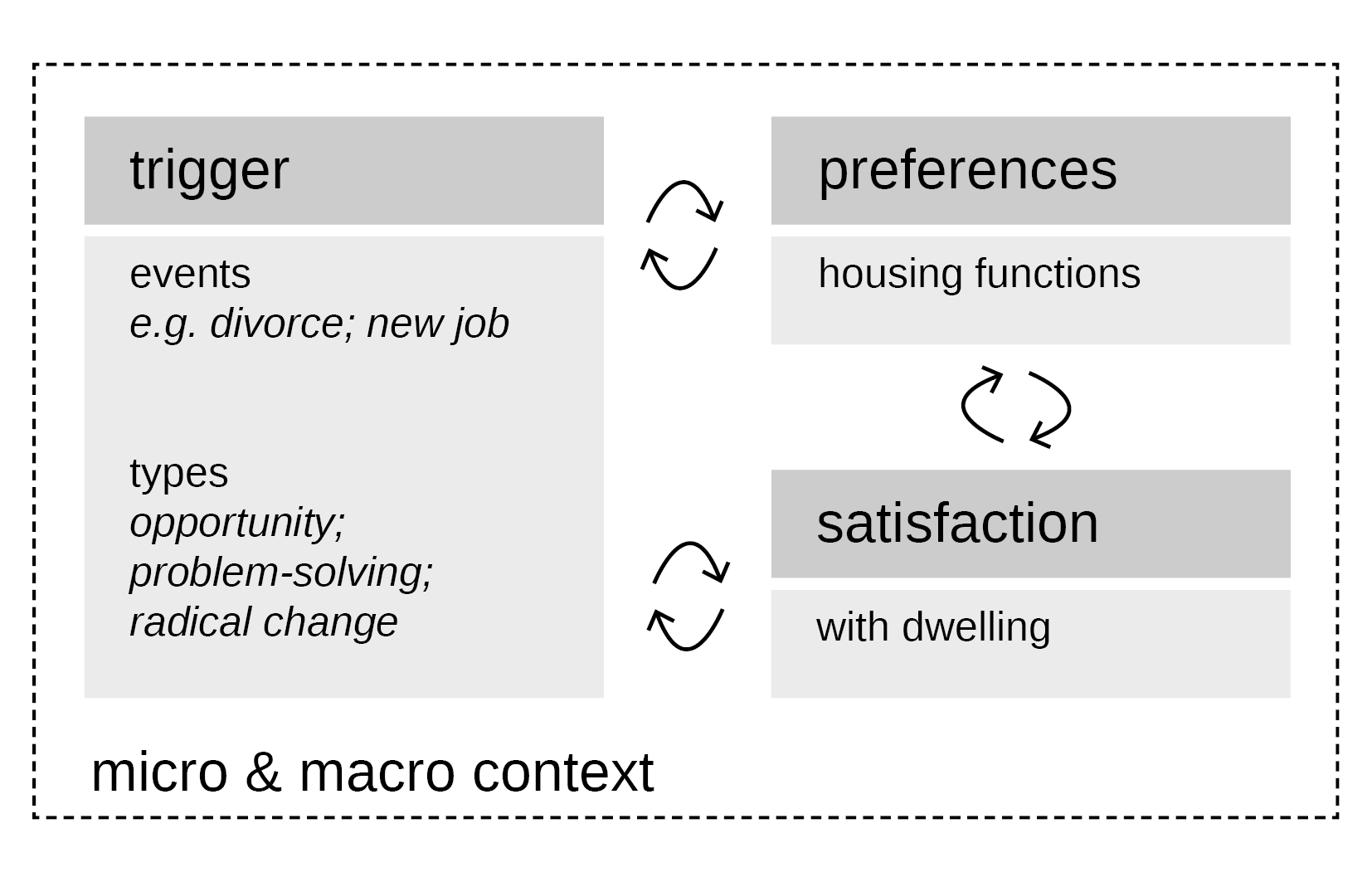
Most of the literature on residential mobility describes it as the process by which a household decides to move and to choose a new dwelling (Dieleman et al. 2000). This process is commonly divided into two stages: in the first, a stressor or trigger arises for the household to decide to seek a new residence; in the second, the household searches, evaluates and selects a housing vacancy based on its residential preferences with the goal of increasing its satisfaction (Brown & Moore 1970; Lu 1998; Mulder 1996; Mulder & Hooimeijer 1999).
Several attempts to model the interactions between triggers, residential preferences and residential satisfaction can be found among existing ABMs (see Huang et al. 2014 and Klabunde & Willekens 2016 for an overview). For instance, the HI-LIFE model uses qualitative and quantitative data to simulate household agents’ (HA) residential mobility in relation to changes in their lifecycle stages (Fontaine & Rounsevell 2009). Following a trigger (e.g., couple formation), the HA’s preferred features are updated according to the HA type, thereby influencing the search for vacancies and their ranking (i.e. via potential attractiveness).
Similarly, other models of residential mobility increasingly distinguish between agent types based on ‘stages’ of a household’s lifecycle (e.g., RESMOBcity by Haase et al. 2010; HRRM by Ma et al. 2013). However, the concept of the ‘lifecycle stage’ has been gradually replaced by the ‘life course’ notion (Ham 2012), which models individual life histories from a succession of micro- and macro-level events linked to a household’s family, education, work, or residential careers (for theory, see Clark & Dieleman 1996; Clark & Lisowski 2017; Mulder & Hooimeijer 1999; Rérat 2020; for examples of computer models, see Klabunde & Willekens 2016; Torrens 2007). These life events can variously affect the preferences of a household for its dwelling (see Devisch et al. 2009; Ettema 2011). Preferences are most often modelled as depending on a feature of interest (e.g., the agent’s religious identity; Benenson et al. 2002) and derived from a bundle of dwelling or location attributes (e.g., neighbourhood identity).
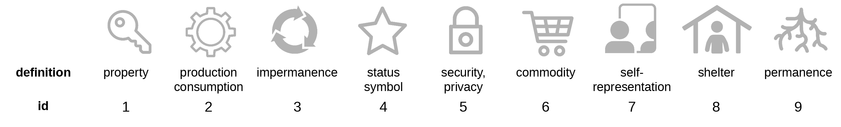
In light of these complex interrelationships, our earlier work conceptualised, explored and operationalised the relocation process by means of a systems perspective (Pagani et al. 2021; Pagani & Binder 2021). To account for the specificities of Swiss housing, we conducted two group discussions and a survey involving 968 tenants of three multifamily housing owners, namely the insurance company and institutional property owner Swiss Mobiliar (Schweizer Mobiliar Asset Management AG), and two of the country’s largest housing cooperatives: ABZ (Allgemeine Baugenossenschaft Zürich) and SCHL (Société Coopérative d’Habitation Lausanne).1 Results showed that triggering events resulting from the progression in a households’ life course career can be categorised into opportunities, problems to solve, and radical changes, whereby depending on its satisfaction with the current location, a household either considers moving or is forced or induced to do so, respectively (Clark & Onaka 1983; Ma et al. 2013). Radical changes were observed to most strongly alter households’ preferences for the new dwelling. Residential preferences were investigated via the notion of housing functions, i.e., what the housing system is for’ (Gero & Kannengiesser 2004; Meadows 2008). Ranging from ‘status symbol’, to ‘permanence’, or ‘commodity’, nine functions of the housing system were identified in the literature and explored empirically. Revealed preferences were studied by looking at the current functions of the dwellings in which households lived and the associated dwelling’s features (e.g., balcony); stated preferences were defined as the functions desired for a dwelling and found to depend on households’ sociodemographic characteristics.2
A decreasing gap between the two types of functions was shown to increase residential satisfaction with the dwelling, which is relevant for both the decision to move and the selection process. In fact, when searching for a new dwelling, the household seeks to make the best possible match between where to live and how it wants to live (Thomas & Pattaroni 2012). This match might be sub-optimal, as the selection of a dwelling depends on households’ preferences within a choice set, which will be widened or narrowed by micro-level resources and restrictions (e.g., financial resources) as well as macro-level opportunities and constraints (e.g., availability of housing and prices, job opportunities; Rérat 2020; Ham 2012; Figure 1).
Agent-Based Model
Having introduced the goal of ReMoTe-S (Section 1) as well as the conceptual system and empirical explorations on which its assumptions are based (Section 2), in this section, we provide an overview of the most important model design decisions structured according to the Overview, Design concepts and Details (ODD) protocol (Grimm et al. 2010; for the full protocol, see Model Documentation).
Entities and state variables
ReMoTe-S introduces four classes of multidimensional agents: tenants, households, dwellings, and buildings. The tenant belongs to a household, who lives in a dwelling contained in a building. Each agent disposes of a unique id number and of state variables that control its behaviour (Table 1; see the ODD protocol for full list).
| State variable | Type | Range | Description | |
|---|---|---|---|---|
| Building | dwellings_num | integer | \([2,121]\) | number of dwellings in the building |
| owners_type | string | {ABZ, SCHL, Mobiliar} | multifamily housing owner | |
| postcode | integer | \([1000, 9000]\) | postcode where the building is located | |
| neighbourhood | set | {safe, sociocultural mix, accessible by car} | ||
| places_of_interest | set | {work, public transports, city centre} | ||
| Dwelling | rooms | integer | \([1, 7]\) | number of rooms in the dwelling |
| size | integer | f(rooms) | dwelling size depending on rooms | |
| rent_price | f(size) | yearly rent price based on dwelling size | ||
| characteristics | set of strings | {bright, with balcony, with green spaces, with parking place} | ||
| functions | set of integers | e.g., {1, 5, 9} | set of functions of the dwelling | |
| Household | mover | boolean | \([0, 1]\) | if True, then agent is searching for a dwelling |
| trigger | string | e.g., ‘divorce’ | trigger to move (see Table 2) | |
| months_waited_ since_mover | integer | \([0, \infty)\) | count of months searching for a dwelling | |
| TYPE | integer | \([1, 13]\) | household type | |
| desired_functions | set of integer | e.g., {1, 5, 9} | set of household’s desired functions | |
| satisfaction | float | [1, 5] | residential satisfaction with the dwelling | |
| Tenant | age | integer | [0,99] | age of the tenant |
| member_type | string | {minor, adult} | under or over 18 years old | |
| salary | float | f(age) | monthly salary depending on age category | |
Building: This agent class is composed of a certain number of dwelling agents that are managed by three different Swiss multifamily housing owners, i.e., ABZ, SCHL and Mobiliar. Buildings are characterised by a postcode depending on the geographical location of the owners’ building stock and by qualitative features, such as closeness to ‘places of interest’ (e.g., public transport) and ‘neighbourhood’ qualities (e.g., safe).
Dwelling: Each dwelling agent comprises a single household agent. Dwellings are characterised by quantitative state variables, e.g., the number of rooms, size, and rent price, and qualitative ones, i.e., ‘characteristics’ (e.g., balcony). Most important for the relocation process is the set of functions (\(F\)) that the dwelling fulfils (e.g., status symbol, shelter, property; see Figure 2).
Household: This class is composed of one or more members i.e., tenant agents. A household agent is characterised by its type (\(T\)), which results from the combination of the average age, number, and type of its members (adults, minors; e.g., \(T8\) = middle-aged couple with children living at home). The agent holds the most relevant state variables for the relocation process, including residential preferences (i.e., its set of desired functions \(DF\); Figure 2), residential satisfaction (min = 1, max = 5), and other variables useful to control its moving behaviour, e.g., the trigger that pushed it to move, the amount of time it spent searching for a dwelling.
Tenant: A household member, i.e., tenant agent, is predominantly characterised by its age and its member type, which determine its monthly salary.
Process overview and scheduling
The process is simulated on a stepwise monthly basis wherein one step represents one month. The initialisation of the model (time-step \(t_{0}\)) is followed by the two sub-models ‘to move’ (\(t_{1}\)) and ‘to select’ (\(t_{2}\)) which are executed successively at each global time step (Figure 3).
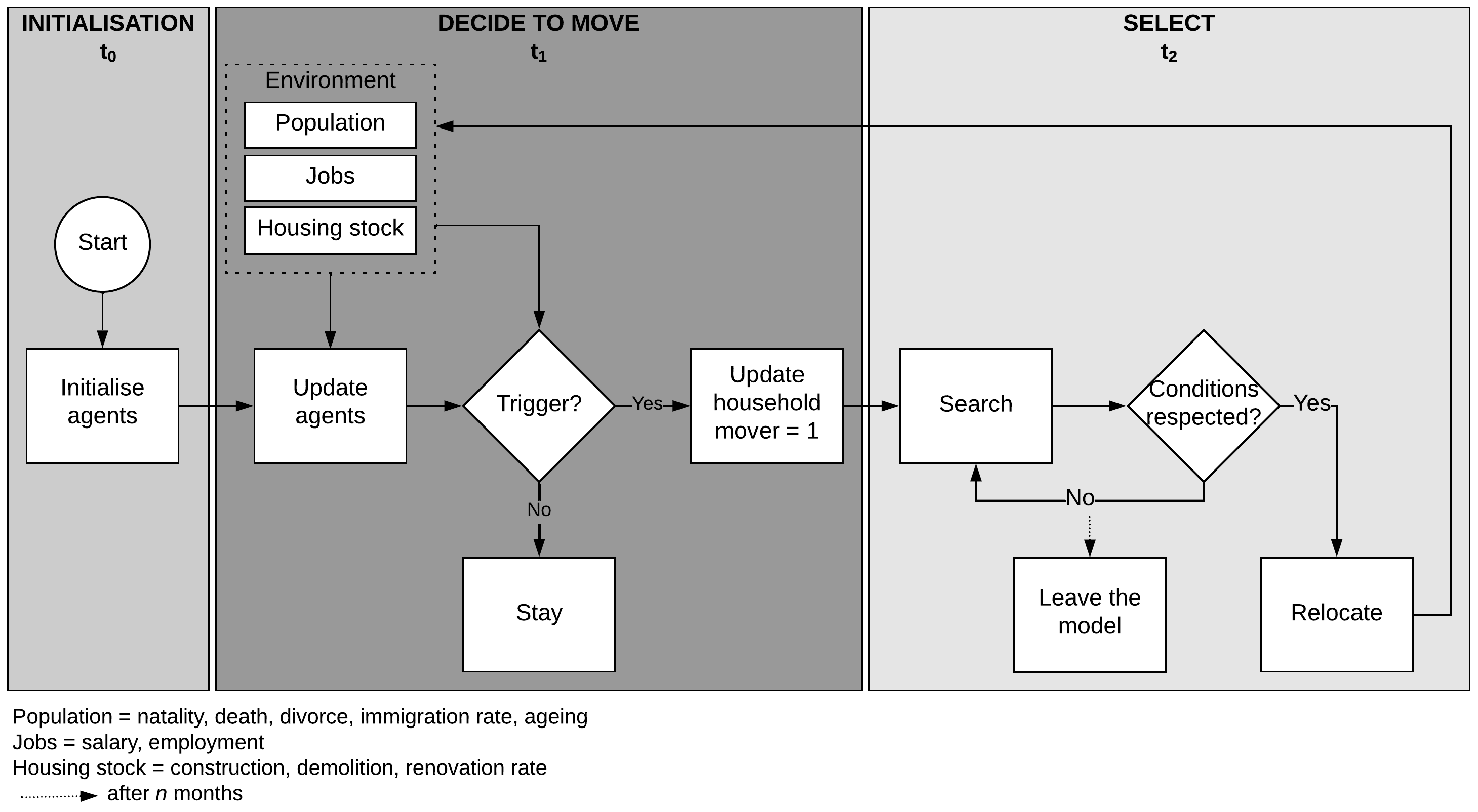
Progress in the family, work and/or residential life course careers can result in a trigger, whereby households are synchronously updated as movers (\(t_{1}\)) and sequentially activated to engage in the search of a new dwelling (\(t_{2}\)). At the end of \(t_{2}\), the movers have either found a dwelling or continue the search. If a suitable vacancy is not found after \(n\) time-steps, we assume that agents out-migrate, i.e., move to dwellings belonging to housing providers other than the three simulated in ReMoTe-S.
Higher-level processes are used to simulate agent dynamics according to global parameters.
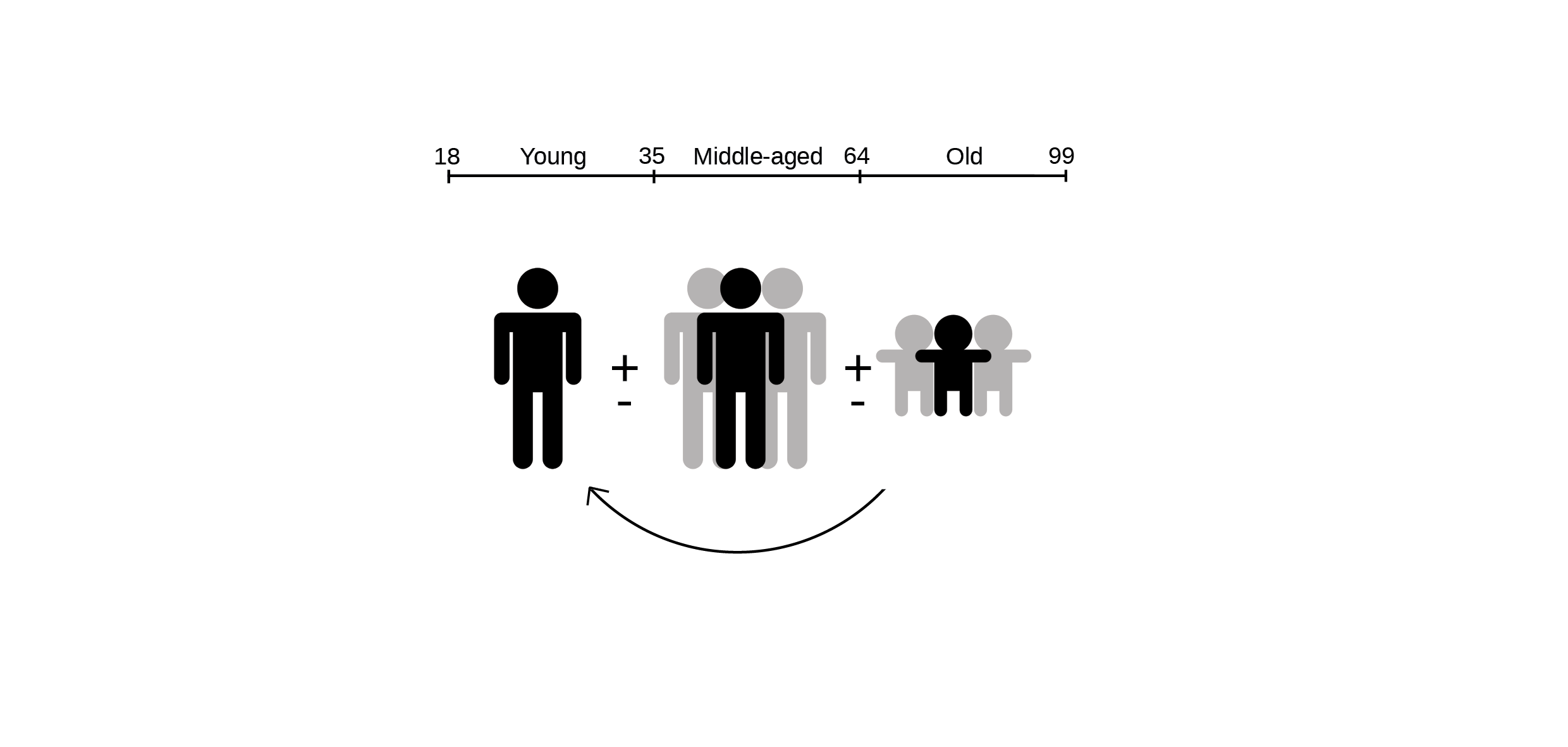
Population: While progressing in age, agents are born, become independent adults, form and dissolve groups (couple, flatshare), have children and die following rules and events compatible with their type (Figure 4). At every time-step, new agents enter the model to search for a vacancy. These processes are regulated by the passing of time (ageing every 12 time-steps), mortality, natality, divorce, and immigration rates. In addition, we assume that households’ residential satisfaction falls by 0.1% with every additional time-step spent in their dwelling (see Friege et al. 2016).
Jobs: The salary and employment status of the tenant agent evolve over time. More specifically, salaries are subjected to a yearly increase of 0.9% unless the tenant is fired and given a subsidy by the state for a maximum of two years (FSO 2019b; SECO 2020).
Housing stock: Dwellings and buildings are affected by construction, demolition, and renovation rates. Dwellings can undergo renovation and be unavailable for a fixed amount of time, following which the rent price is adjusted. We assume that buildings are demolished depending on their age and the amount of time their dwellings have been vacant.
Design concepts
This subsection concisely describes four of the design concepts proposed by Grimm et al. (2010), which are relevant for understanding how ReMoTe-S works.
Objectives: Based on the theoretical framework introduced in Section 2, we assume that household agents’ final goal is to find a dwelling that maximises residential satisfaction under supply constraints and households’ restrictions. Our empirical explorations revealed that the gap between residential aspirations and reality is a predictor of residential satisfaction (Pagani et al. 2021). Therefore, the level of satisfaction of a household agent \(i\) with a dwelling \(j\) at time \(t\) (\(los_{ij}(t)\)) is calculated based on the correspondence of its set of desired functions to the set of functions of the selected dwelling:
| \[ los_{ij}(t) = 4 (\frac{len(DF_{i} \& F_{j})}{len(DF_{i})}) + 1\] | \[(1)\] |
For instance, if at time \(t\) \(DF_{i}=\{1, 3, 5, 8\}\) and \(F_{j}=\{1, 3, 7\}\), the resulting satisfaction is:
| \[ los_{ij}(t) = 4 (\frac{2}{4}) + 1 = 3\] | \[(2)\] |
Interaction: In the moving process, agents directly and indirectly interact within and across classes. Examples of direct interactions include: a tenant’s loss of job, which affects the salary of its collective (tenant-household); the merging of two households, e.g., via couple formation (household-household); or more simply renting or leaving a flat (household-dwelling). Occupying a dwelling can also have indirect effects by preventing similar agents from finding a vacancy that satisfies them and eventually pushing them to leave the model (i.e., competition).
Stochasticity: Stochasticity is used to simulate the random component for which an agent would decide to move in a particular period, i.e., to cause model events to occur and trigger residents’ relocation following empirically based probabilities (e.g., a change in job location; see Section 4.6). Stochasticity also serves to reproduce variability in processes whose cause is irrelevant (e.g., the sample of dwellings that an agent ‘sees’ when searching; Grimm et al. 2010).
Observation: The desired information is collected at every time step and saved in a .csv file at the end of the simulation. The output data are then sampled and used for testing, understanding and analysing the model’s behaviour, as illustrated in the following sections.
Model Initialisation and Input Data
The model is populated with the tenants’ survey dataset (\(N = 878\)). The dataset contains information on households’ socio-demographic characteristics (including e.g., types, salary), their revealed and stated preferences (i.e., desired/current housing functions, housing features), the triggers that pushed them to relocate, and their residential satisfaction. When needed, statistics from the Federal Statistical Office (FSO) are used instead. The initialisation process does not vary among simulations; however, stochastic variables vary with every iteration.
Agents are initialised via three procedures. A desired number of buildings is first generated (\(N = 30\)). The buildings’ owner type corresponds to the share of survey respondents per owner (ABZ = 33.5%, SCHL = 39.5%, Mobiliar = 27%), based on which the postcode is assigned. Buildings are randomly attributed at least one qualitative feature among ‘neighbourhood’ and ‘places of interest’.
Secondly, dwellings are created and distributed among available buildings. The distribution of the number of rooms per dwelling is based on survey data (\(M = 3.5\), \(SD = 1\)) and is used to determine the dwelling’s size (sqm/room) and rent price (CHF/sqm). Dwellings are stochastically attributed a minimum of one ‘characteristic’. The set of functions (\(F\)) of a dwelling agent is established with probabilities that depend on dwellings’ and buildings’ features in the survey (see Table 7 in Appendix).
Finally, households are generated (\(N = 1000\)). Their type (\(T\)) follows the distribution of survey respondents and is used to set the ranges of several tenant agents’ state variables (e.g. age, salary). The set of desired functions (\(DF\)) is sampled from their frequencies per household type in the survey (see Table 8 in Appendix).
The initialisation process works similarly to the process ‘select’ (\(t_{2}\)) and consists of matching households to available dwellings depending on a set of conditions. The process is completed when all dwellings are occupied. A fixed number of vacant dwellings is then randomly generated in existing buildings in order to comply with the rental housing vacancy rate of different Swiss cantons (0.4% for postcode 1000, 0.1% for postcode 8000, 2.7% for all others; Wüest Partner 2020).
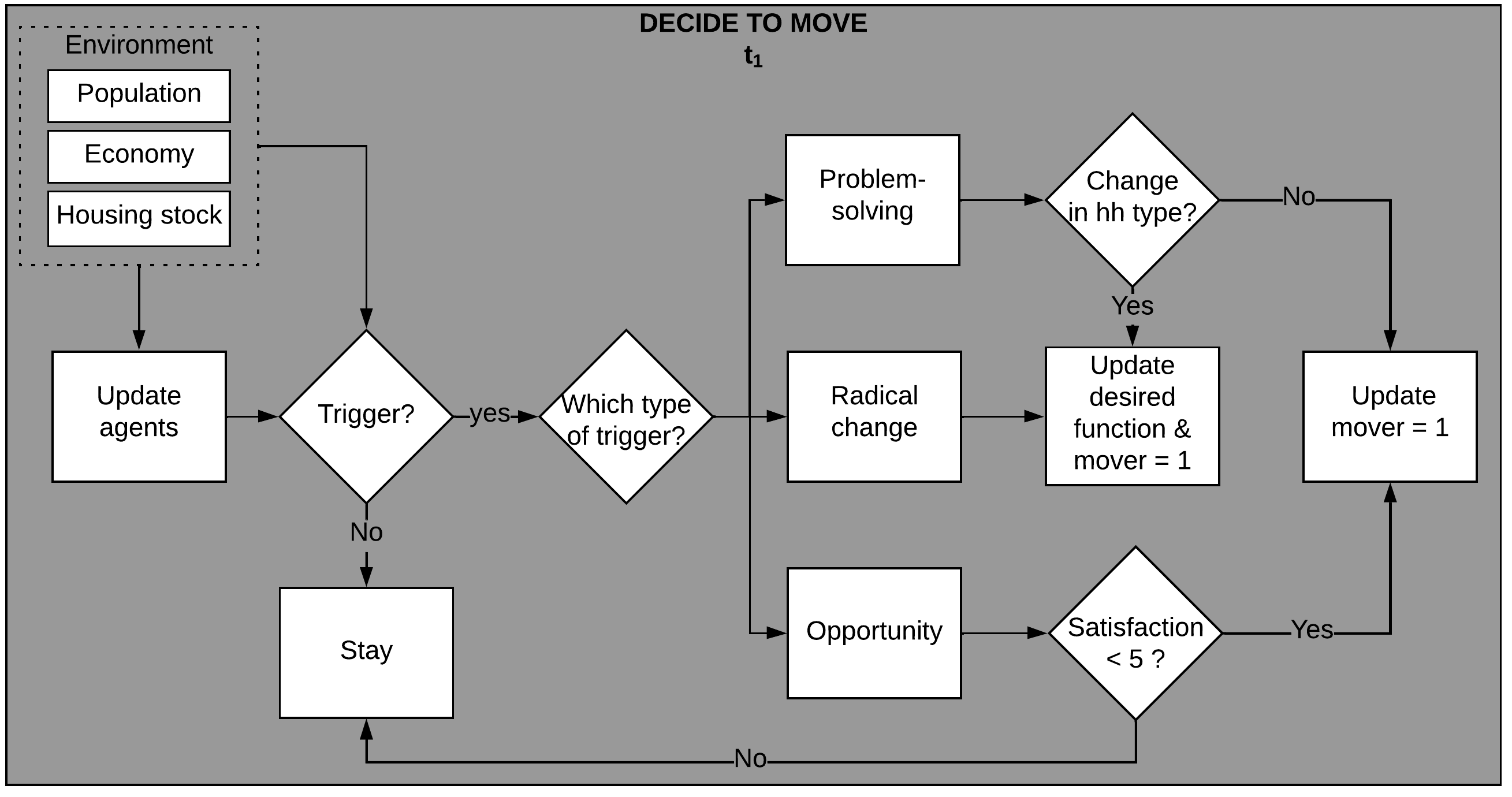
Decide to move
This subsection illustrates the first sub-model of ReMoTe-S, at the end of which household agents decide to move (Figure 3 and Figure 5).
We consider 17 triggers organised in the three types identified in our previous qualitative and quantitative exploratory work (Pagani et al. 2021; Pagani & Binder 2021): opportunities, which are effective under the condition of a medium level of satisfaction (i.e., \(< 5\)); problems to solve; and radical changes (Table 2).
| Opportunity | Problem-solving | Radical change |
|---|---|---|
| 1. Salary increase | 3. Expire contract | 11. Change job location |
| 2. New building\(^{a}\) | 4. Demolition | 12. Need for change |
| 5. Renovation / transformation | 13. Create couple | |
| 6. Interpersonal problems | 14. New child | |
| 7. Rent too high | 15. Separate / divorce | |
| 8. Underoccupancy | 16. Children leaving | |
| 9. Growing old, retirement | 17. Leaving the flatshare | |
| 10. Family\(^{b}\) | ||
Triggers are discrete events caused by either the environment (i.e., exogenous) or a sequence of events in the model (i.e., endogenous). The probabilities of exogenous triggers to occur are based on the survey dataset and official statistics. Endogenous triggers depend instead on parallel events (e.g., the loss of a job can render the rent unaffordable). Certain requirements must be met for an event to trigger a household’s move; for instance, the expiration of rental contract does not apply to cooperative tenants, whereas underoccupancy checks do not apply to non-cooperative housing.3
Synchronously with radical changes and changes in household’s type, the household agent is attributed a new set of desired functions (i.e., update in residential preferences).
Select
Following the process ‘decide to move’, agent-movers are sequentially activated to search for either joinable groups or vacant dwellings (Figure 6). Values are updated as soon as they are calculated by the process (i.e., asynchronous updating) so that the dwellings that have been occupied first are not available for the next searching agent.
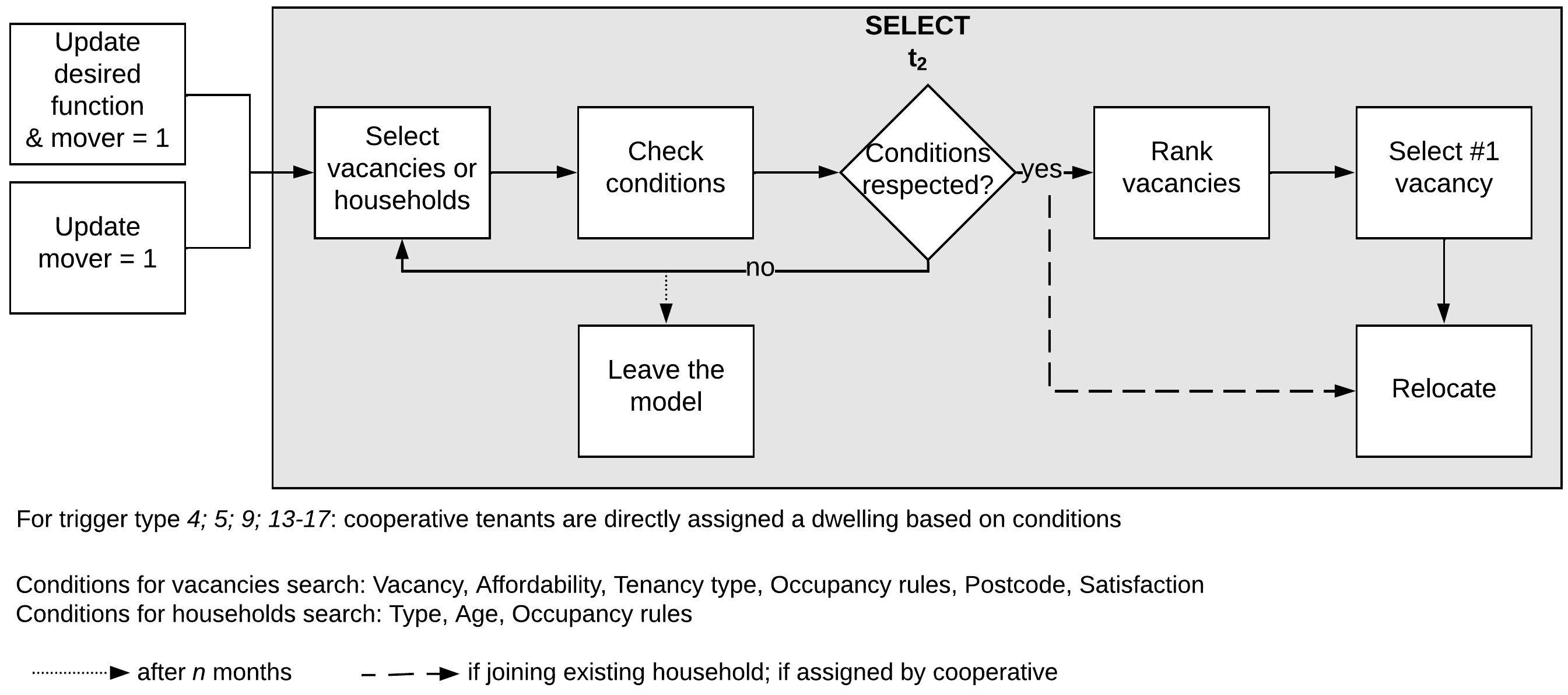
We assume that the household (i) filters the dwellings it ‘sees’ depending on a set of ‘conditions’ (Table 3), (ii) gathers them in a list, (iii) ranks them according to the satisfaction they potential generate, and eventually (iv) moves to the first one on the list. If two alternatives have the same score, then the dwelling is randomly selected; if no dwelling is found in \(n\) time-steps, then the household out-migrates.
| Condition | Description | Process |
|---|---|---|
| Vacancy | The dwelling is empty. | \(t_{0}\), \(t_{2}\) |
| The dwelling is different from that where the household resides. It is not under renovation and will neither be demolished nor renovated in the following year. | \(t_{2}\) | |
| Affordability | \(SA_{i}(t) \geq 1/3 R_{j}(t)\), where \(SA_{i}(t)\) is the sum of the annual salary of each member comprising the household \(i\) and \(R_{j}(t)\) is the annual rent of the selected dwelling \(j\). | \(t_{0}\), \(t_{2}\) |
| Tenancy type | For SCHL and ABZ: the selected dwelling belongs to the same owner as the current one. | \(t_{2}\) |
| Occupancy rules | Mobiliar: \(S_{i}(t) -1 \leq RO_{j}(t) \leq S_{i}(t) + 2\) SCHL and ABZ: \(S_{i}(t) -1 \leq RO_{j}(t) \leq S_{i}(t) + 1\), where \(S_{i}(t)\) is number of members of the household \(i\) and \(RO_{j}(t)\) is the number of rooms of the selected dwelling \(j\) at time \(t\). |
\(t_{0}^{a}\), \(t_{2}\) |
| Postcode | It must be equal to the postcode of the current dwelling, except in case of a change in job location (trigger 11) or the need to move closer to the family (trigger 10). | \(t_{2}\) |
| Satisfaction | \(los_{ij}(t) \geq los_{ik}(t)\), where \(los_{ik}(t)\) is the level of satisfaction of a household \(i\) with its current dwelling \(k\) at time \(t\), and \(los_{ij}(t)\) is the level of satisfaction with the selected dwelling \(j\) (see Equation 1). | \(t_{0}\), \(t_{2}\) |
In the case of a divorce or when leaving the flatshare, the household engages in the search for a joinable group, for which we establish the following rules: (i) the household must not be in a couple; (ii) it must include a tenant who is maximum 10 years older/younger than the searching one; and (iii) for flatshares only, there must be space for a new tenant (i.e., occupancy rules; Table 3).
If a single partner is found, then the newly-formed couple will look for a new dwelling to which to move; if a flatshare is found, then the tenant will be directly integrated in their dwelling; if the tenant has not found a compatible household to join after a fixed number of attempts, then s/he will create a one-person household and search for a vacancy for 1-time step.
Model Calibration and Verification
The model’s calibration and verification are part of a circular process (Boero & Squazzoni 2005), which we synthetize in two steps. First, we set the baseline scenario by adjusting one key parameter to produce a desirable output value (Fontaine & Rounsevell 2009; Friege et al. 2016; Palmer et al. 2015; Schulze et al. 2017). Second, we follow a household agent over its life course to verify whether the model performs as expected.
We account for the stochastic variation of parameter values by evaluating the outputs of 100 simulation runs via averages and confidence intervals (Huang et al. 2014). To estimate the model’s long-term behaviour, the time span is set to 30 years (i.e., 360 time-steps; see Hatna & Benenson 2015).
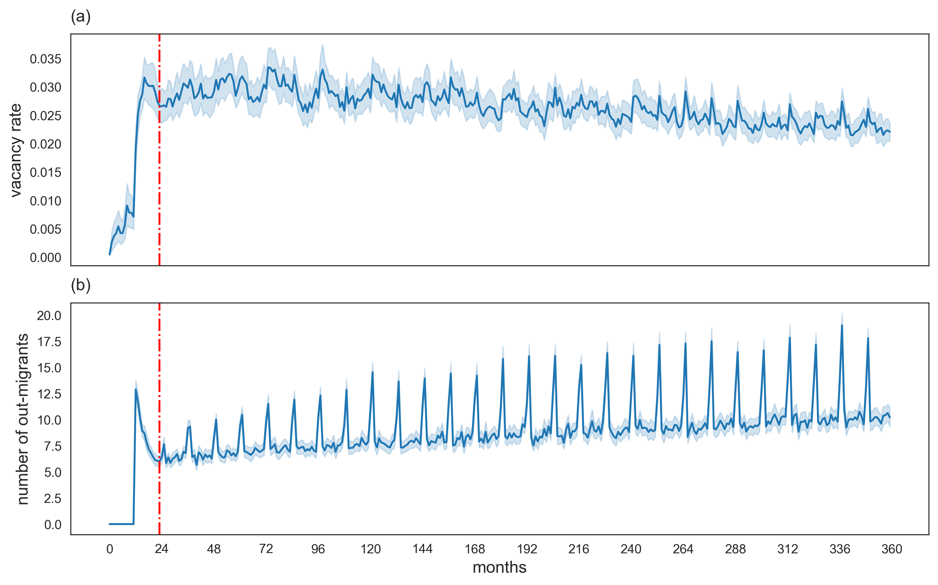
Setting the baseline scenario
A key characteristic of the Swiss housing market is its remarkably low vacancy rate (Thalmann 2012; Werczberger 1997). Considering that ReMoTe-S simulates households’ in- and out-migration, this rate is greatly influenced by the number of agents who try to enter the model monthly. Therefore, the parameter ‘immigration rate’ is calibrated by varying its value between 0% and 10% and selecting the best fit of the output to the average Swiss dwelling vacancy rate (2.7% in 2019; Wüest Partner 2020). After filtering out the effects of the model ‘warm up’ (23 time-steps; Figure 7), a final value of 4% of monthly immigration rate is retained as the closest to real-world data.
Following a household over its life course
Although ABMs enable the investigation of both micro- and macro-level outcomes, the model verification and validation rarely include individual-level observations (Huang et al. 2014). Figure 8 schematically synthetises the .csv output of one of 100 model runs, whereby selected metrics are recorded over 30 years of simulation to observe a household’s job, family and housing careers and eventually its out-migration.
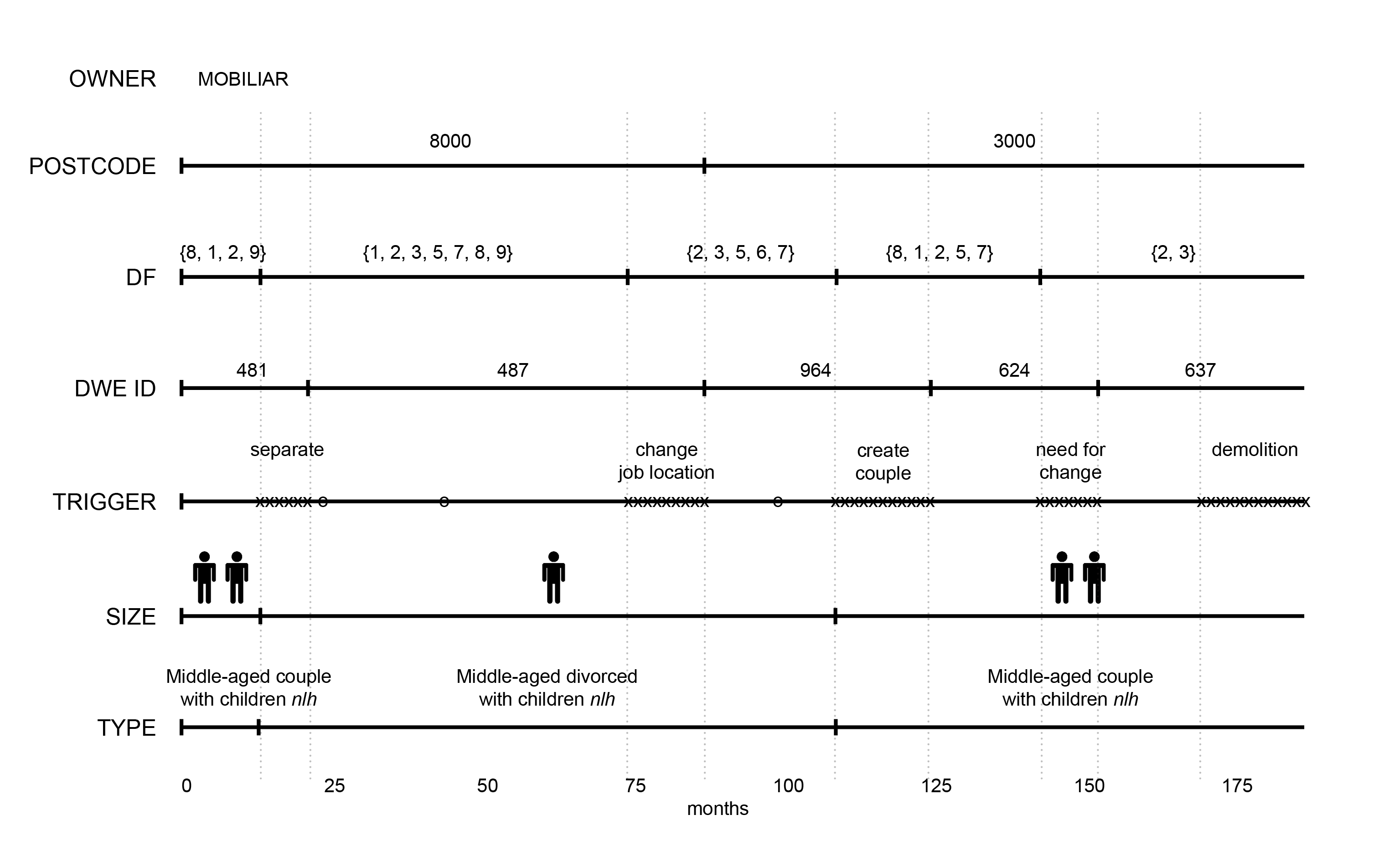
Following a separation, one of the two household’s members remains in the dwelling and engages in the search for a new one (for a maximum of 12 time-steps), whereas the other former partner immediately leaves the shared accommodation to search for potential joinable groups. This event, which corresponds to a radical change, updates the household’s preferences, meaning that a new set of desired functions is computed based on its new type (i.e., divorced). After approximately five years, a change in job location triggers the search for a dwelling in a different postcode than the current one (i.e., 3000). Three years later, the agent receives the trigger ‘create couple’, meaning that its state variables have aligned with the constraints of another tenant in search of a joinable group. Towards the end of the simulation, the household is notified of the upcoming demolition of the building it inhabits. An unsuccessful search pushes it to out-migrate. Over its time in ReMoTe-S, new buildings are generated in the same postcode where the agent resides; however, its attempts to obtain a new dwelling fail (i.e., another agent occupies it first).
Simulation Experiments and Scenario Comparison
Following the model’s calibration, simulation experiments are run under the assumption that households’ behaviours and demographic trends continue as they are today. The purpose of the experiments is to observe the sensitivity of model outputs to changes in dwellings’ qualitative and quantitative features. The impacts of these variations are monitored via two key indicators of housing sustainability: (i) average floor space per capita, which is the largest determinant of domestic energy consumption; and (ii) average vacancy rate, which provides information on whether dwelling features exhaustively fulfil households’ preferences (Table 4).
| Exp | Scenario | Rooms | Features | Indicators |
|---|---|---|---|---|
| Parameters varied | Parameters varied | |||
| 1\(^{a}\) | Baseline | M = 3.5 | min = 2, max = 10 | sqm/tenant |
| SD = 1.0 | Full palette | #tenants in three rooms | ||
| min = 1, max = 10 | #one-person household | |||
| S1 | M = 1.5 | baseline | ||
| SD = 1.0 | ||||
| min = 1, max = 10 | ||||
| 2\(^{b}\) | A3 | Baseline | min = 2, max = 3 | vacancy rate (new dwellings, all dwellings) |
| With green spaces | #dwelling functions | |||
| Close to PT | level of satisfaction | |||
| Sociocultural mix | ||||
| B7 | baseline | min = 2, max = 7 | ||
| Bright, with balcony, with parking place | ||||
| Close to work, close to city-center | ||||
| Safe, accessible by car | ||||
| B3 | baseline | min = 2, max = 3 | ||
| With parking place | ||||
| Close to work | ||||
| Accessible by car | ||||
| A7 | baseline | min = 2, max = 7 | ||
| Bright, with balcony, with green spaces | ||||
| Close to PT, close to city-center | ||||
| Safe, sociocultural mix | ||||
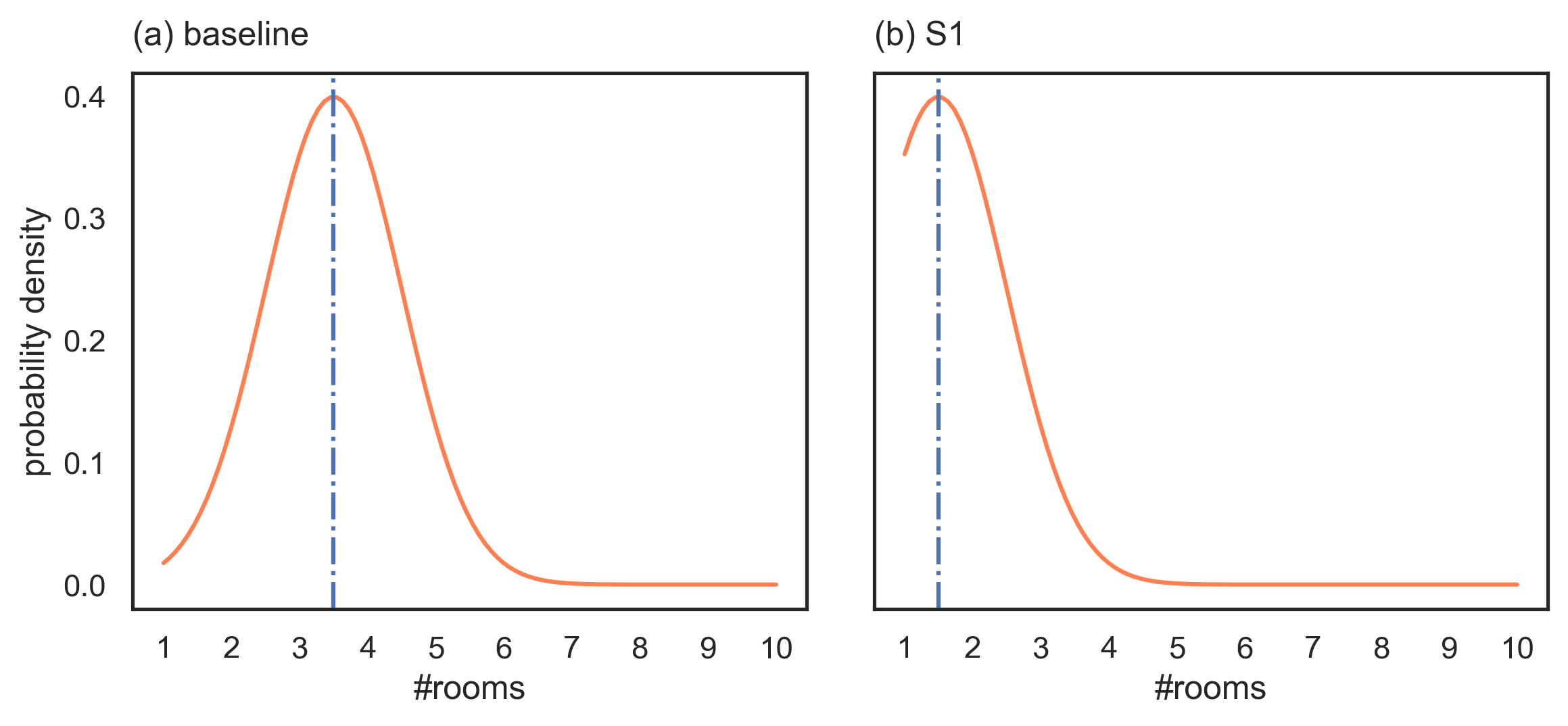
The first experiment explores the impact of changes in average dwelling size on how efficiently dwellings are occupied. A one-factor-at-a-time sensitivity analysis (OFAT) is run on the parameter ‘rooms mean’ (\(M\)),4 which controls the average number of rooms per dwelling (initialised and newly built) in the housing stock. We then specifically focus on two scenarios with a larger number of medium- (baseline; Figure 9a) and small-size dwellings (S1; Figure 9b).
The second experiment explores and compares the effects of the provision of new housing with ‘sustainable’ and ‘unsustainable’ features on the average dwellings’ vacancy rate, which is assumed to depend on households’ satisfaction and therefore on the number of housing functions per dwelling (Equation 1). For this purpose, we reduce the palette of ‘characteristics’, ‘neighbourhood’ and ‘places of interest’ that can be randomly attributed to dwelling and building agents when newly built (i.e., not at initialisation; minimum one feature per agent class). Scenarios A3 and B3 can be characterised by a maximum of three ‘sustainable’ and ‘unsustainable’ features, respectively; the complementary scenarios B7 and A7 can generate dwellings with all features except the three ‘sustainable’ and ‘unsustainable’ ones, respectively (Table 4). Finally, we check the sensitivity of the scenarios’ results to changes in construction rate (set to 0.69%). The model warm-up is fixed at 47 months, the time span during which the output ‘new dwellings available rate’ shows the largest fluctuation.
Experiment 1: The impact of dwellings’ size on floor area per capita
Figure 10a illustrates the sensitivity of the output ‘sqm/tenant’ to changes in the parameter ‘rooms mean’. We observe that the area per capita increases as the average number of rooms per dwelling increases up to 3.5 rooms on average, beyond which it is relatively stable. This result indicates a positive correlation between the number of small dwellings in the housing stock and the efficiency of space usage.
If we compare the provision of medium-size (baseline) with that of small-size dwellings (S1, Figure 10b), we observe that the difference in floor area per capita is particularly accentuated in three-room apartments. Considering that this size represents the largest majority of dwellings in our sample (baseline; Figure 9a), the overall efficiency of space use appears to predominantly depend on how well three-room apartments are occupied.
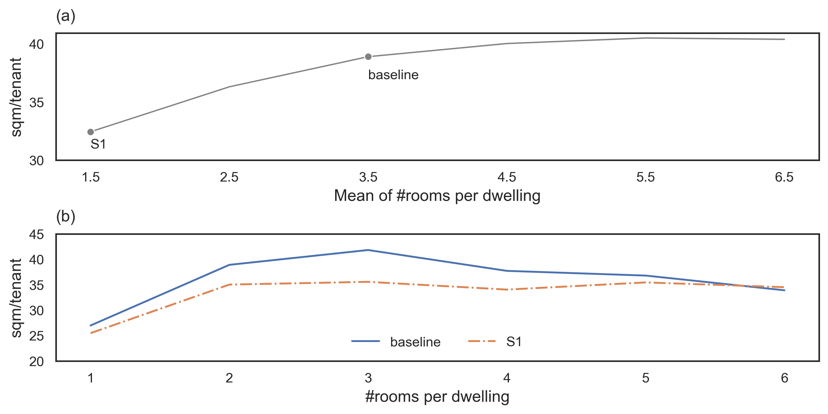
Figure 11a illustrates the occupation of these dwellings for two housing providers: the cooperative ABZ and the asset manager Mobiliar. We observe that when the average size is centred between 3.5–5.5 rooms, the number of tenants occupying a three-room apartment is overall the lowest. It therefore appears that when the offer of smaller dwellings is reduced, tenants tend to under-occupy medium-to-large dwellings.
This hypothesis is reinforced by Figure 11b, which compares the number of one-person households renting from the two housing owners. In the case of the cooperative, we observe that the number of single households in the model decreases with a decreasing supply of smaller dwellings (i.e., with a greater average number of rooms). In contrast, we observe that for the asset manager, there is little-to-no difference between the number of one-person households in a scenario with smaller (mean = 1.5; S1) and those with average-size dwellings (mean = 3.5; baseline).
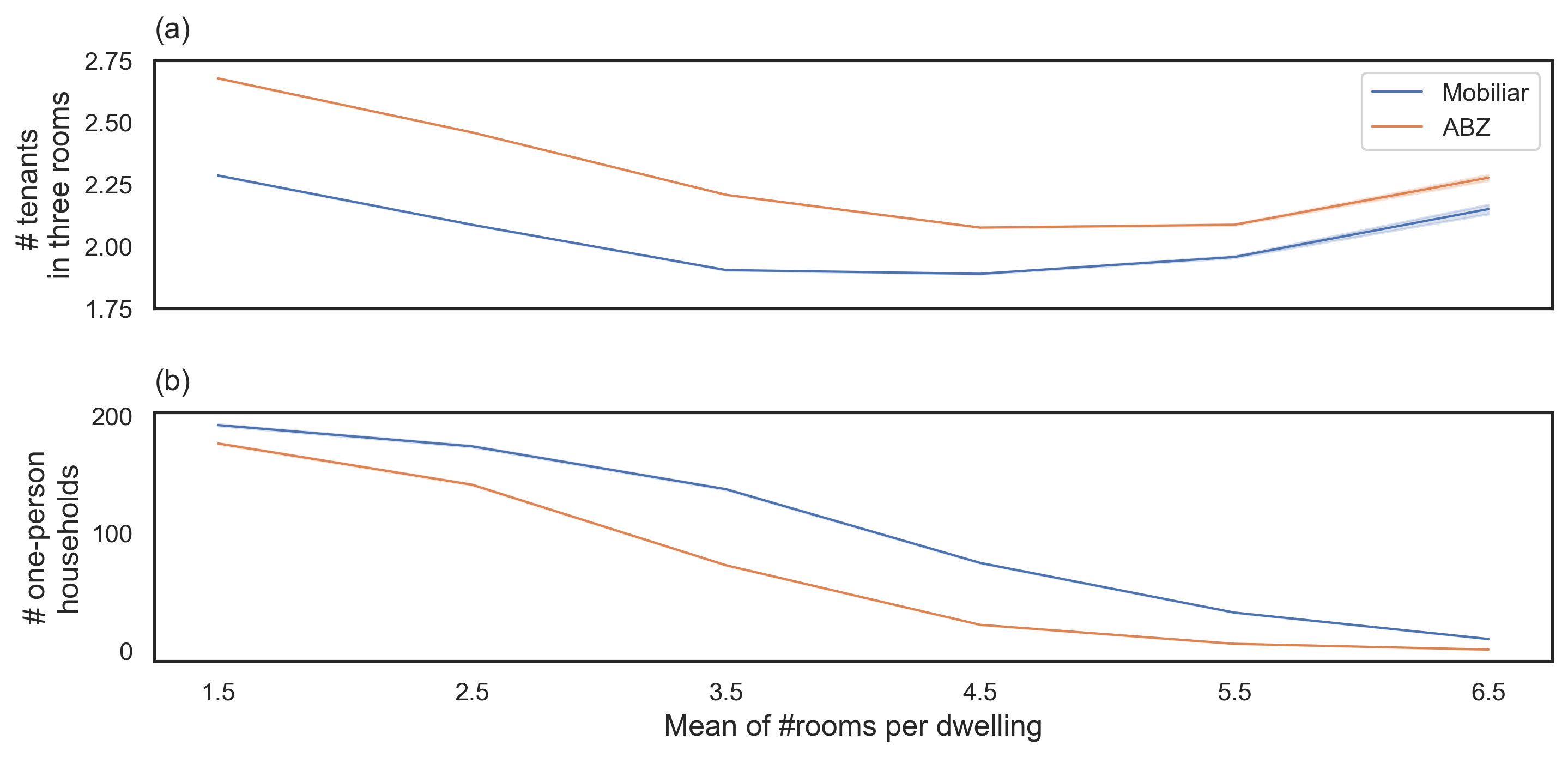
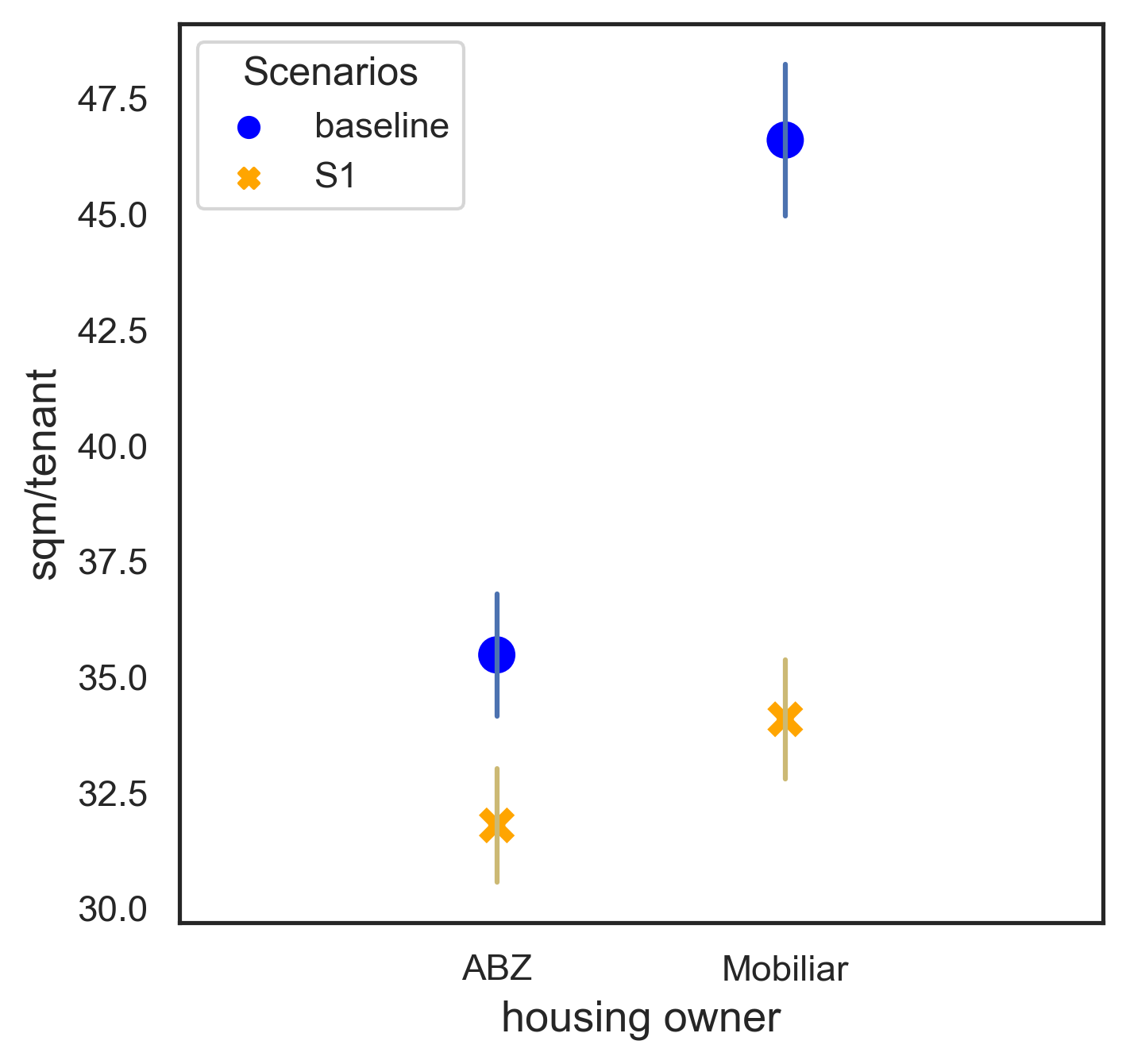
Figure 12 provides additional information on the indicator ‘sqm/tenant’ for ABZ and Mobiliar, whereby as per occupancy rules, the latter exhibits the most space-consuming tenants (baseline; Table 3). Notably, a provision of smaller dwellings has the largest effect on the occupancy of its dwellings (baseline M = 46.6, SD = 1.63; S1 M = 34.1, SD = 1.28), which becomes comparable to the one of the cooperative ABZ (baseline M = 35.5, SD = 1.32; S1 M = 31.8, SD = 1.22). This result can be explained by the occupancy rules set for the households of Mobiliar, which allow a relocating tenant to occupy a three-room dwelling alone (versus two rooms for the cooperatives). This behaviour is also supported by the relative affluence of ReMoTe-S tenants, who can afford larger dwellings on their own.
In summary, results indicate that a reduced supply of small-size dwellings and a greater flexibility in occupancy rules result in an increase of floor area per capita.
Experiment 2: The success of ‘sustainable’ housing features
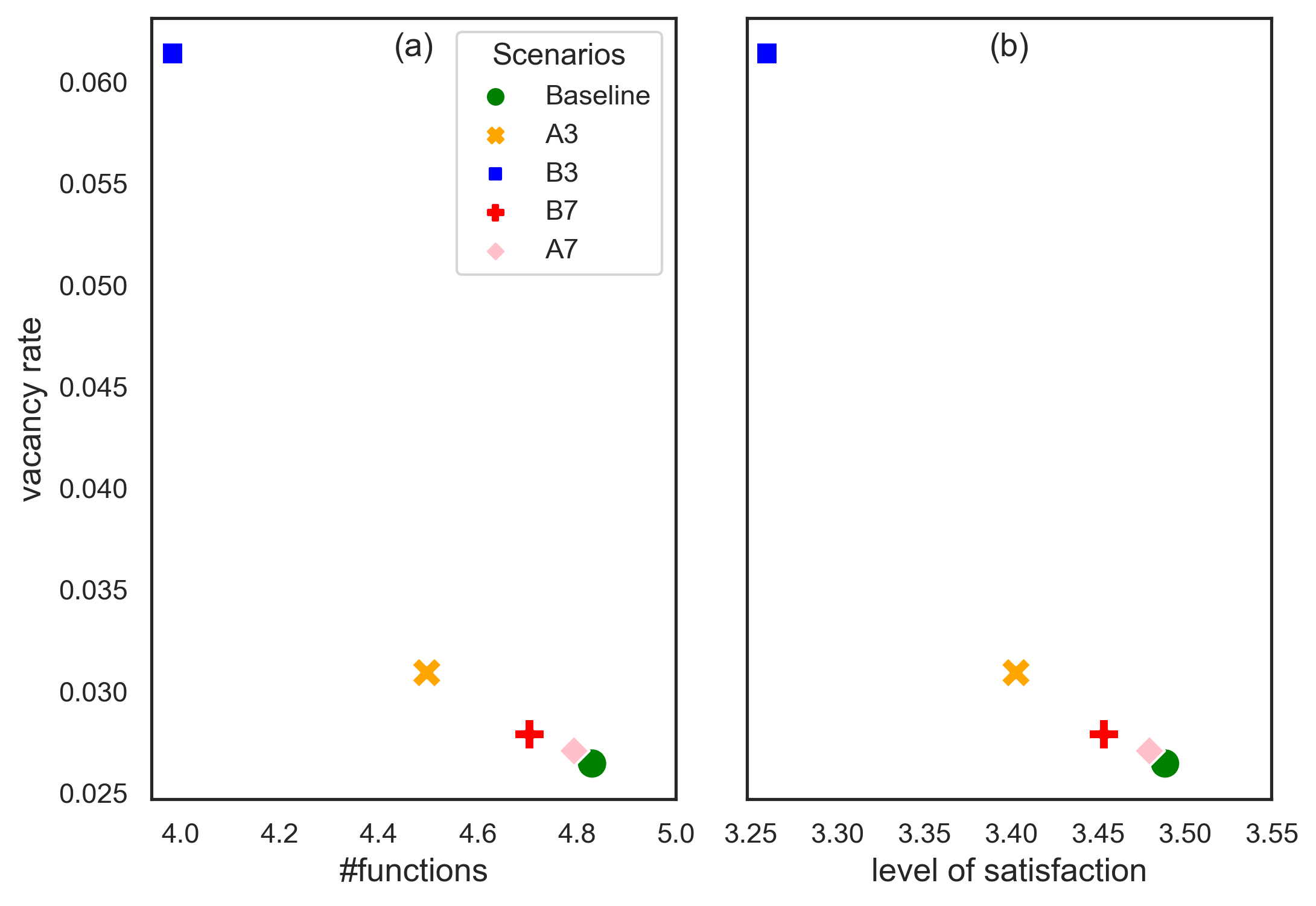
Figure 13 displays the dwellings’ average vacancy rate for the five scenarios described in Table 4.
When comparing the two sub-figures, we observe a positive correlation between the number of functions fulfilled by a dwelling and the household population’s level of satisfaction. When comparing the scenarios with three features (A3, B3) and seven features (A7, B7), we also observe that a larger number of possible features entails on average a larger number of dwelling functions. These results are coherent with model rules, whereby satisfaction depends on the match between the functions of the desired and selected dwellings, the latter of which is computed based on their characteristics, proximity to places of interests and neighbourhood qualities. However, the difference between the two ‘sustainable’ housing scenarios A3 and A7 in all indicators is negligible compared with the difference between the ‘unsustainable’ scenario B3 and all others. If we also consider that the vacancy rate for scenario A3 (with only three features) is very close to that for B7 (with seven features), then the results seem to suggest that scenario A3 includes characteristics that are comparably more relevant for generating functions, and thus satisfaction.
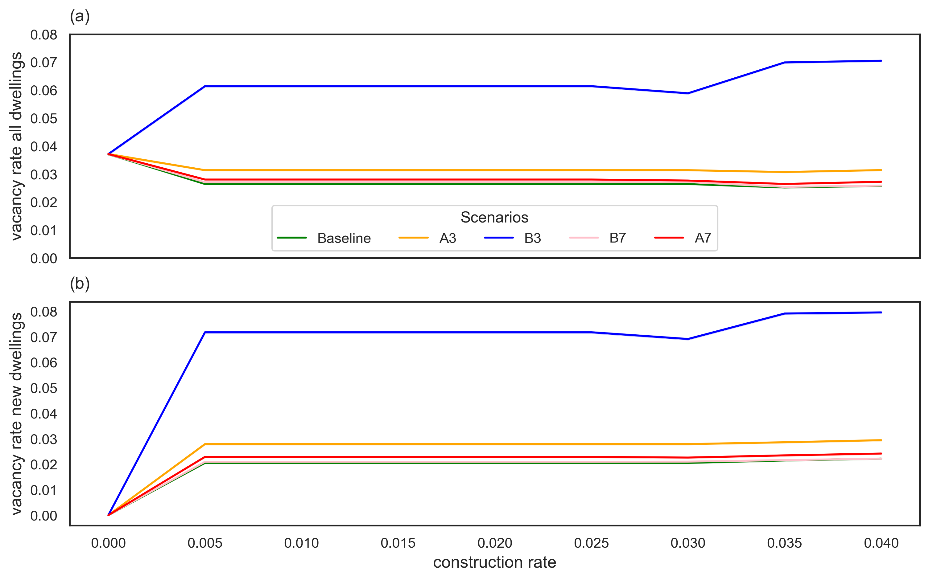
To investigate whether the results are sensitive to the number of new dwellings generated during the simulation, Figure 14 shows the results of the OFAT on the construction rate parameter for the five scenarios. Overall, the plots corroborate our observations, in that the relative difference in vacancy rates does not vary with an increase of new dwellings. Furthermore, we observe that from a 0.5% construction rate onwards, the vacancy rate of all dwellings (Figure 14a) and new dwellings (Figure 14b) is relatively small and stable for most scenarios. This result would indicate that the larger the number of attractive dwellings, the larger the number of households (in the model and in-migrating) that find a suitable vacancy in the housing stock. Conversely, the scenario B3 exhibits a considerably large vacancy rate, which increases with greater construction rates. This finding confirms that the dwellings provided in B3 mismatch with the desired functions of the majority of the simulated households. It also suggests that, from a construction rate of 3%, the number of newly-constructed dwellings exceeds the (small) share of households with matching preferences and requirements.
Discussion and Conclusion
This paper addressed the need of Swiss property owners to navigate the complexity of the housing system to provide both environmentally and socio-culturally sustainable dwellings. We outlined an approach for modelling the recursive effects between households and dwellings, which are made explicit in residential mobility. We based our agent-based model on explicit assumptions derived from a survey of tenants of three Swiss housing providers and illustrated its utility through two applications. While accounting for context-specific factors that are determinant to the relocation process, the model responds to the need for more empirically-based and context-specific ABMs (Boero & Squazzoni 2005; Knoeri et al. 2011).
Below, we first put the results of the simulations in perspective and discuss the validity and limitations of the ABM. We then conclude with practical recommendations for the three housing providers and propose avenues for future research.
Results in perspective
To outline potential uses of the model, we focused on two relevant aspects of housing sustainability: (i) housing size (monitored via sqm/tenant) and (ii) preferences for and success of certain housing features (via vacancy rate, satisfaction). This exploration entailed simultaneously considering households’ preferences, satisfaction and triggers to move as well as opportunities and constraints (e.g., dwellings available) and resources and restrictions (e.g., household salary), all of which ReMoTe-S was designed to include.
The goal of Experiment 1 was to explore the effects of variations in dwellings’ average size on individual space consumption. It emerged that a supply that prioritises medium-to-large size dwellings in combination with a less strict application of occupancy rules can result in an increase in average floor area per capita. This finding is in agreement with other studies (Ellsworth-Krebs 2020; Huebner & Shipworth 2017) and in particular with the statistical analyses of Karlen et al. (2021), which were conducted with the same survey dataset used in this article. Karlen et al. (2021) highlighted the lack of an adequate supply of small dwellings for the increasing number of one- and two-person households as well as the absence of occupancy rules or rigor in enforcing them as obstacles to reducing space consumption. Furthermore, and also in line with our results, a preference for larger dwellings was found to especially concern tenants with sufficient financial resources.
Experiment 2 aimed at achieving a better understanding of the effect of changing dwelling, neighbourhood, and location features on dwelling vacancy rates by observing variations in the functions they fulfil and households’ residential satisfaction. Our findings are key to research on residential mobility more generally as well as more specifically on the discrepancy and reciprocal influence between stated and revealed preferences (Clark & Dieleman 1996; Clark & Lisowski 2017; Dieleman 2001; Mulder & Hooimeijer 1999). In fact, we demonstrated that dwelling and building features only determine whether a dwelling fulfils one or more housing functions to a certain extent and with interesting combinations. As previously argued by the authors (Pagani et al. 2021), and in line with other scholars (Lawrence 1987; Michelson 1980), residential satisfaction is not based on the ‘mechanistic’ correspondence between the set of desired and current characteristics of the settlement (e.g., balcony, public transports). Simulating the mediating effects of housing functions makes it possible to account for the trade-offs in the relative value attached to specific dwelling, neighbourhood and location features (Rapoport 2000).
Model validity
Before discussing its validity, the purpose of a model and its level of complicatedness need to be stated (Edmonds et al. 2019; Sun et al. 2016). Considering the seven categories proposed by Edmonds et al. (2019), ReMoTe-S was developed for a descriptive purpose; it represents ‘what is important’ in the relocation process of a subpopulation of Swiss tenants renting from three housing owners. Thus, the ABM lies on a spectrum between a toy model and a ‘complicated’ model with a higher degree of structural realism (Schulze et al. 2017; Sun et al. 2016). A minority of ABMs of residential dynamics make the validation process explicit by demonstrating the plausibility of the assumptions underlying the model (i.e., conceptual validation; Knoeri et al. 2011), or its initial conditions (see Fontaine & Rounsevell 2009; Friege et al. 2016; Torrens 2007). On these premises, we discuss model validity as follows.
Concerning conceptual validation, the implementation of ReMoTe-S is the outcome of a structured transdisciplinary research path that entailed the formulation of an interdisciplinary conceptual model, its qualitative exploration in group discussions, and its quantification in a survey with the tenants of three multifamily housing owners. Its operating rules, boundaries and input data can be considered reasonable because they were based on and agreed upon by the decision-makers it simulates (Janssen & Ostrom 2006).
Concerning the plausibility of the model outputs, the households’ average salary, satisfaction, number of desired functions and triggers to move were checked for their correspondence to survey results across all modelling stages (i.e., implementation, initialisation; for more information, see the ODD protocol). In addition, the plausibility of micro-level outputs was verified by collecting and analysing 100 different residential mobility patterns of one agent over its life course. Lastly, the sensitivity analyses presented in this paper enabled us to explore extreme model conditions (e.g., 0% of immigration rate) as well as discuss and interpret the emergent effects of our manipulations.
Limitations
The most relevant limitations of ReMoTe-S concern the assumptions on which the model is built as well as the dataset, methods, and choice of experiments.
The focus of our empirical investigations on tenants’ residential mobility required us to formulate assumptions on the dynamics of the housing stock, i.e., construction, demolition, renovation. Although the difference between cooperative and non-cooperative housing was accounted for, heterogeneity in e.g., cantonal regulations were levelled out by using data at the scale of the confederation. Furthermore, the occupancy rules matching households to dwellings require further investigation, as their real-world application may sometimes be less strict than was simulated in the ABM (Karlen et al. 2021)5.
The survey dataset also has certain limitations. In particular, the data used to attribute functions to dwellings shows relatively small differences across features’ frequencies for a given dwelling function (see Table 7 in Appendix). However, the choice not to vary this distribution was consciously taken in line with the goal to account for preferences in the closest alignment with the reality depicted by the survey.
Concerning the methods, our choice of an OFAT sensitivity analysis enabled our interdisciplinary research team to have equal control and understanding over the varied parameters and the emergent system responses. However, its simplicity and attractiveness expose its limitations, which could be overcome by exploring other approaches (see Lee et al. 2015; ten Broeke et al. 2016).
Regarding the choice of experiments, the selection of building and dwelling features to include and exclude in Experiment 2 was based on an artificial dichotomy drawn between ‘sustainable’ and ‘unsustainable’ dwellings. It should be acknowledged that depending on contextual and normative factors, the characteristics of the ‘unsustainable’ scenarios might well be perceived as sustainable (e.g., a parking place can be essential for a family with children attending school in another neighbourhood). Furthermore, Experiment 1 should also be considered as an exploration of artificial conditions in that the dwellings of scenario S1 cannot accommodate large households.
It is also worth mentioning that the relatively high degree of realism of ReMoTe-S and its context dependency inevitably bring about less generality (Knoeri et al. 2011), and the results therefore need to be contextualised and carefully discussed.
Recommendations and future research
Bearing these limitations in mind, we would like to propose recommendations for the three housing providers simulated in ReMoTe-S, based on which we outline future research pathways targeting a sustainable management of the residential building stock.
To reduce per capita floor space, the projected increase in the number of one-person households in Switzerland (FSO 2019c) should be counteracted by the supply of a greater number of small dwellings and the adoption of occupancy rules by all housing providers. This measure is especially relevant considering that the majority of the Swiss housing stock was composed of three- or four-room apartments in 2019, whereas one-room apartments represented only 6% (FSO 2019a). In the same vein, additional measures could be explored in future experiments. For instance, to prevent tenants from forming one-person households as a consequence of an unsuccessful search for a joinable flatshare, age limits for the formation of groups could be varied, such as by permitting young students to mix with elderly tenants in intergenerational dwellings. Furthermore, variations in the standard deviation of the number of rooms per dwelling (fixed to 1; Table 4) could enable the investigation of the effects of a more diversified housing supply capable of accommodating any household size.
The provision of sustainable housing understood in all its dimensions must also account for the potential discrepancy between the dwellings’ objectively measurable qualities and inhabitants’ subjective perception of them. In particular, we encourage housing providers to consider that a design based on a perfect correspondence between stated and revealed preferences for housing features (e.g., preference for parking places = design of more parking places) underestimates the complexity of trade-offs aimed at fulfilling needs at a higher systemic level, which ReMoTe-S can help to address. Applications of this knowledge should be supported by more research on the association between functions and dwelling, neighbourhood, and location features in different socio-cultural contexts.
To conclude, we invite scholars to focus on one or more aspects of ReMoTe-S to address new research questions. In addition, the model could be integrated with an ABM simulating the housing market (e.g., rent evolution), to provide a more accurate instrument to identify and promote practical measures for a sustainable management of the residential building stock.
Model Documentation
ReMoTe-S is implemented in the open-source software Python 3.9. The code and the ODD protocol linked to this paper are available from CoMSES OpenABM at this link: https://www.comses.net/codebase-release/45117bff-8627-4ab9-a4e4-bb26e79a662e/.Acknowledgements
This research is part of the project “Shrinking Housing’s Environmental Footprint (SHEF)”, supported by the Swiss National Science Foundation (SNSF) within the framework of the National Research Programme “Sustainable Economy: resource-friendly, future-oriented, innovative” (NRP 73) under Grant [number 407340_172435]. The authors would like to acknowledge Swiss Mobiliar Cooperative Company, project partner and funder of the Swiss Mobiliar Chair in Urban Ecology and Sustainable Living, the Laboratory for Human-Environment Relations in Urban Systems (HERUS), as well as the housing cooperatives SCHL and ABZ and their tenants for their collaboration. Also, they would like to thank the organisers and participants of ESSA@work for their comments and suggestions on ReMoTe-S. In particular, they acknowledge Dr. Bastian Wilding for the feedback given at all stages of the modelling process and the manuscript preparation. The authors especially thank the two anonymous reviewers and the journal editor for their constructive and valuable comments.Notes
- Collectively, these owners manage approximatively 10,000 dwellings. The sample size used for analyses was N = 878.↩︎
- Our previous work introduced the concept of ‘desired’ function as an adaptation of the ‘ideal’ function to micro-level resources and restrictions (e.g., a household’s income), whereas the ‘current’ function is described as an adaptation of the desired function to macro-level opportunities and constraints (e.g., available dwellings; Pagani et al. 2021). As agent-based modelling permits us to account for the interaction between micro- and macro-level factors, this paper focuses on the simulation of ‘desired’ functions and ‘current’ functions—here simply defined as ‘dwelling’ functions. To do so, we applied the empirical knowledge gained on the notion of ideal functions to that of desired functions, assuming a linear effect of the gap between aspirations and reality on households’ satisfaction (Equation 1).↩︎
- This trigger consists of an annual check of the cooperatives’ (i.e., ABZ, SCHL) compliance rules with the goal to prevent inefficient use of space. This rule only applies to the cooperative dwellings with \(RO_{j}(t) \geq 4\) and if \(S_{i}(t)<RO_{j}(t) – 2\), where \(RO_{j}(t)\) is the number of rooms for a dwelling \(j\) at time \(t\), and \(S_{i}(t)\) is the number of members of a household \(i\) at time \(t\).↩︎
- OFAT entails selecting ‘a base parameter setting […] and varying one parameter at a time while keeping all other parameters fixed’ (ten Broeke et al. 2016, p. 3).↩︎
- The average floor area per capita in the model is smaller than in our empirical sample. However, the difference between cooperative and non-cooperative housing is well captured, which is why the model setup can be used to compare them (for more details on this limitation, see Section 7.1 of the ODD protocol).↩︎
Appendix
This section provides additional information on the dataset used for the model parametrisation.
| T | Description | Age | Size | % |
|---|---|---|---|---|
| 1 | young single\(^{a}\) | 18-35 | S1 = 1A to 10A | 5 |
| 2 | young couple\(^{b}\) without children | 18-35 | S2 = 2A | 8.5 |
| 3 | young couple with children | 18-35 | S3 = 2A + 1M to 8M | 3 |
| 4 | young alone\(^{c}\) with children | 18-35 | S4 = S3 -1A | 0.6 |
| 5 | middle-aged single\(^{a}\) | 36-64 | S5 = 1A to 10A | 10.3 |
| 6 | middle-aged couple without children | 36-64 | S6= 2A | 7.7 |
| 7 | middle-aged alone without children | 36-64 | S7 = 1A | 6.9 |
| 8 | middle-aged couple with children living at home | 36-64 | S8 = 2A + 1M to 8M | 19 |
| 9 | middle-aged couple with children not living at home | 36-64 | S9 = 2A | 5.4 |
| 10 | middle-aged alone with children living at home | 36-64 | S10 = S8 –1A | 5.8 |
| 11 | middle-aged alone with children not living at home | 36-64 | S11 = 1A | 4.4 |
| 12 | older couple (with/without children) | 65-99 | S12 = 2A + 1M to 8M | 11.1 |
| 13 | older alone\(^{c}\) (with/without children) | 65-99 | S13 = 1A to 10A or S12-1A | 12.1 |
| TOT | 100 | |||
| Parameter | N | State variable | Source | ||
|---|---|---|---|---|---|
| Buildings | num_buildings | 30 | assumption | ||
| dwellings (#) | random | assumption | |||
| owner type | survey | ||||
| ABZ | 33.5% | ||||
| SCHL | 39.5% | ||||
| Mobiliar | 27% | ||||
| postcode | SCHL = 1000, ABZ = 8000, Mobiliar = random | survey | |||
| age | \([0-40]\) | assumption | |||
| neighbourhood\(^{a}\) | random | assumption | |||
| places of interest\(^{a}\) | random | assumption | |||
| Dwellings | num_dwellings | 1000 | survey | ||
| rooms | M = 3.5, SD = 1.0, min = 1, max = 10 | survey | |||
| size | f(rooms) | FSO\(^{b}\) | |||
| rent_price | f(size) | FSO\(^{b}\) | |||
| characteristics\(^{a}\) | random | assumption | |||
| function | see Table 7 | survey | |||
| Households | num_households | 1000 | survey | ||
| TYPE | see Table 5 | survey | |||
| members | |||||
| #children | M = 1.67, SD = 0.76, min = 1, max = 5 | survey | |||
| #adults in flatshare | Type = 1, M = 1.49, SD = 1, min = 1, max = 6 Type = 5, M = 1.17, SD = 0.57, min = 1, max = 4 |
survey | |||
| Type = 13, M = 1.12, SD = 0.48, min = 1, max = 5 | |||||
| desired functions | see Table 8 | survey | |||
| satisfaction | 3 | assumption\(^{b}\) | |||
| Tenants | age | f(TYPE) | FSO\(^{b}\) | ||
| salary | f(age) | FSO\(^{b}\) | |||
| Dwelling and building features | F1 | F2 | F3 | F4 | F5 | F6 | F7 | F8 | F9 | |
|---|---|---|---|---|---|---|---|---|---|---|
| Dwelling | % | % | % | % | % | % | % | % | % | |
| bright | 24 | 24 | 27 | 21 | 21 | 24 | 26 | 24 | 25 | |
| with balcony | 38 | 39 | 34 | 33 | 36 | 38 | 38 | 39 | 39 | |
| with green spaces | 26 | 29 | 28 | 29 | 30 | 26 | 30 | 29 | 30 | |
| with parking place | 16 | 19 | 17 | 20 | 20 | 19 | 17 | 17 | 13 | |
| Places of interest | work | 33 | 33 | 27 | 27 | 32 | 31 | 29 | 32 | 28 |
| close to... | public transports | 49 | 53 | 52 | 37 | 54 | 55 | 52 | 52 | 53 |
| city-centre | 31 | 33 | 35 | 38 | 33 | 33 | 35 | 33 | 35 | |
| Neighbourhood | safe | 39 | 31 | 31 | 33 | 31 | 31 | 31 | 32 | 32 |
| sociocultural mix | 24 | 23 | 21 | 16 | 22 | 25 | 22 | 25 | 23 | |
| accessible by car | 17 | 24 | 24 | 20 | 24 | 26 | 22 | 23 | 18 | |
| DF1 | DF2 | DF3 | DF4 | DF5 | DF6 | DF7 | DF8 | DF9 | |
|---|---|---|---|---|---|---|---|---|---|
| % | % | % | % | % | % | % | % | % | |
| T1 | 94 | 94 | 50 | 22 | 28 | 44 | 67 | 83 | 50 |
| T2 | 77 | 97 | 41 | 13 | 41 | 26 | 62 | 97 | 74 |
| T3 | 89 | 100 | 56 | 33 | 67 | 22 | 78 | 100 | 67 |
| T4 | 100 | 100 | 100 | 0 | 100 | 100 | 100 | 100 | 0 |
| T5 | 85 | 100 | 30 | 11 | 56 | 26 | 70 | 85 | 67 |
| T6 | 71 | 96 | 46 | 14 | 54 | 18 | 61 | 82 | 61 |
| T7 | 67 | 100 | 56 | 11 | 78 | 33 | 67 | 100 | 44 |
| T8 | 63 | 100 | 25 | 19 | 53 | 13 | 66 | 97 | 72 |
| T9 | 57 | 100 | 43 | 0 | 43 | 29 | 29 | 57 | 57 |
| T10 | 67 | 100 | 50 | 0 | 58 | 42 | 58 | 67 | 33 |
| T11 | 60 | 100 | 100 | 0 | 80 | 60 | 100 | 80 | 80 |
| T12 | 58 | 100 | 54 | 4 | 67 | 29 | 38 | 79 | 67 |
| T13 | 50 | 94 | 61 | 6 | 56 | 33 | 50 | 83 | 61 |
References
BENENSON, I. (2004). 'Agent-Based modeling: From individual residential choice to urban residential dynamics.' In M. F. Goodchild & G. Janelle (Eds.), Spatially Integrated Social Science: Examples in Best Practice (pp. 67–95). Oxford: Oxford University Press.
BENENSON, I., Omer, I., & Hatna, E. (2002). Entity-based modeling of urban residential dynamics: The case of Yaffo, Tel Aviv. Environment and Planning B: Planning and Design, 39(4), 491–512. [doi:10.1068/b1287]
BINDER, C. R., Wyss, R., & Massaro, E. (2020). Sustainability Assessments of Urban Systems. Cambridge, MA: Cambridge University Press. [doi:10.1017/9781108574334]
BOERO, R., & Squazzoni, F. (2005). Does empirical embeddedness matter? Methodological issues on agent-Based models for analytical social science. Journal of Artificial Societies and Social Simulation, 8(4), 6: https://www.jasss.org/8/4/6.html.
BOOI, H., & Boterman, W. R. (2020). Changing patterns in residential preferences for urban or suburban living of city dwellers. Journal of Housing and the Built Environment, 35, 93–123. [doi:10.1007/s10901-019-09678-8]
BROWN, L. A., & Moore, E. G. (1970). The intra-urban migration process: A perspective. Geografiska Annaler: Series B, Human Geography, 52(1), 1–13. [doi:10.1080/04353684.1970.11879340]
CHIU, R. L. H. (2004). Socio-cultural sustainability of housing: A conceptual exploration. Housing, Theory and Society, 21(2), 65–76. [doi:10.1080/14036090410014999]
CLARK, W. A. V. (2012). 'Residential mobility and the housing market.' In D. F. Clapham, W. A. V. Clark, & K. Gibb (Eds.), The SAGE Handbook of Housing Studies (pp. 66–83). London: SAGE Publications. [doi:10.4135/9781446247570.n4]
CLARK, W. A. V., & Dieleman, F. (1996). Households and housing: Choice and outcomes in the housing market. Rutgers - The State University of New Jersey: Centre for Urban Policy Research.
CLARK, W. A. V., & Lisowski, W. (2017). Decisions to move and decisions to stay: Life course events and mobility outcomes. Housing Studies, 32(5), 547–565. [doi:10.1080/02673037.2016.1210100]
CLARK, W. A. V., & Onaka, J. L. (1983). Life cycle and housing adjustment as explanations of residential mobility. Urban Studies, 20(1), 47–57. [doi:10.1080/713703176]
DEVISCH, O. T. J., Timmermans, H. J. P., Arentze, T. A., & Borgers, A. W. J. (2009). An agent-based model of residential choice dynamics in nonstationary housing markets. Environment and Planning A, 41(8), 1997–2013. [doi:10.1068/a41158]
DIELEMAN, F. M. (2001). Modelling residential mobility; a review of recent trends in research. Journal of Housing and the Built Environment, 16, 249–265.
DIELEMAN, F. M., Clark, W. A. V., & Deurloo, M. C. (2000). The geography of residential turnover in twenty-seven large US metropolitan housing markets, 1985-95. Urban Studies, 37(2), 223–245. [doi:10.1080/0042098002168]
EDMONDS, B., Le Page, C., Bithell, M., Chattoe-Brown, E., Grimm, V., Meyer, R., Montañola-Sales, C., Ormerod, P., Root, H., & Squazzoni, F. (2019). Different modelling purposes. Journal of Artificial Societies and Social Simulation, 22(3), 6: https://www.jasss.org/22/3/6.html. [doi:10.18564/jasss.3993]
ELLSWORTH-KREBS, K. (2020). Implications of declining household sizes and expectations of home comfort for domestic energy demand. Nature Energy, 5(1), 20–25. [doi:10.1038/s41560-019-0512-1]
ETTEMA, D. (2011). A multi-agent model of urban processes: Modelling relocation processes and price setting in housing markets. Computers, Environment and Urban Systems, 35(1), 1–11. [doi:10.1016/j.compenvurbsys.2010.06.005]
FONTAINE, C. M., & Rounsevell, M. D. A. (2009). An agent-based approach to model future residential pressure on a regional landscape. Landscape Ecology, 24(9), 1237–1254. [doi:10.1007/s10980-009-9378-0]
FRIEGE, J., Holtz, G., & Chappin, E. J. L. (2016). Exploring homeowners’ insulation activity. Journal of Artificial Societies and Social Simulation, 19(1), 4: https://www.jasss.org/19/1/64.html. [doi:10.18564/jasss.2941]
FSO. (2017). Swiss Federal Statistical Office - Housing Conditions. Retrieved February 15, 2021, from: https://www.bfs.admin.ch/bfs/en/home/statistics/construction-housing/dwellings/housing-conditions.html.
FSO. (2019a). Swiss Federal Statistical Office - Construction and Housing. Retrieved July 13, 2020, from: https://www.bfs.admin.ch/bfs/en/home/statistics/construction-housing/dwellings.html.
FSO. (2019b). Swiss Federal Statistical Office - Evolution des Salaires. Retrieved February 15, 2021, from: https://www.bfs.admin.ch/bfs/fr/home/statistiques/travail-remuneration/salaires-revenus-cout-travail/evolution-salaires.html.
FSO. (2019c). Swiss Federal Statistical Office - Population. Retrieved April 18, 2021, from: https://www.bfs.admin.ch/bfs/de/home/statistiken/bevoelkerung/stand-%0A47%0Aentwicklung/haushalte.html.
GERO, J. S., & Kannengiesser, U. (2004). The situated function-behaviour-structure framework. Design Studies, 25(4), 373–391. [doi:10.1016/j.destud.2003.10.010]
GRIMM, V., Berger, U., DeAngelis, D. L., Polhill, J. G., Giske, J., & Railsback, S. F. (2010). The ODD protocol: A review and first update. Ecological Modelling, 221(23), 2760–2768. [doi:10.1016/j.ecolmodel.2010.08.019]
HAASE, D., Lautenbach, S., & Seppelt, R. (2010). Modeling and simulating residential mobility in a shrinking city using an agent-based approach. Environmental Modelling & Software, 25(10), 1225–1240. [doi:10.1016/j.envsoft.2010.04.009]
HAM, M. van. (2012). 'Housing behaviour.' In D. F. Clapham, W. A. V. Clark, & K. Gibb (Eds.), The SAGE Handbook of Housing Studies (pp. 47–65). London: SAGE Publications.
HATNA, E., & Benenson, I. (2015). Combining segregation and integration: Schelling model dynamics for heterogeneous population. Journal of Artificial Societies and Social Simulation, 18(4), 15: https://www.jasss.org/18/4/15.html. [doi:10.18564/jasss.2824]
HUANG, Q., Parker, D. C., Filatova, T., & Sun, S. (2014). A review of urban residential choice models using agent-based modeling. Environment and Planning B: Planning and Design, 41(4), 661–689. [doi:10.1068/b120043p]
HUEBNER, G. M., & Shipworth, D. (2017). All about size? – The potential of downsizing in reducing energy demand. Applied Energy, 186(2017), 226–233. [doi:10.1016/j.apenergy.2016.02.066]
IEA. (2018a). CO2 emissions from fuel combustion. Retrieved from: https://www.iea.org/subscribe-to-data-services/co2-emissions-statistics.
IEA. (2018b). World energy balances. Retrieved from: https://www.iea.org/subscribe-to-data-services/world-energy-balances-and-statistics.
JANSSEN, M. A., & Ostrom, E. (2006). Empirically based, agent-based models. Ecology and Society, 11(22). [doi:10.5751/es-01861-110237]
KARLEN, C., Pagani, A., & Binder, C. R. (2021). Obstacles and opportunities for reducing dwelling size to shrink the environmental footprint of housing: Tenants’ residential preferences and housing choice. Journal of Housing and the Built Environment. [doi:10.1007/s10901-021-09884-3]
KLABUNDE, A., & Willekens, F. (2016). Decision-Making in agent-Based models of migration: State of the art and challenges. European Journal of Population, 32(1), 73–97. [doi:10.1007/s10680-015-9362-0]
KNOERI, C., Binder, C. R., & Althau, H. J. (2011). An agent operationalization approach for context specific agent-Based modeling. Journal of Artificial Societies and Social Simulation, 14(2), 4. [doi:10.18564/jasss.1729]
LAWRENCE, R. J. (1987). Housing, Dwellings and Homes: Design Theory, Research and Practice. Hoboken, NJ: John Wiley & Sons.
LAWRENCE, R. J. (2009). 'L’attractivité du logement: Notion fédératrice pour saisir la complexité du marché immobilier.' In L. Pattaroni, V. Kaufmann, & A. Rabinovich (Eds.), Habitat en Devenir: Enjeux Territoriaux, Politiques et Sociaux du Logement en Suisse (pp. 225–244). Lausanne: PPUR.
LAWRENCE, R. J., & Barbey, G. (2014). Repenser l’Habitat: Donner un Sens au Logement. Paris: Gollion.
LEE, J. S., Filatova, T., Ligmann-Zielinska, A., Hassani-Mahmooei, B., Stonedahl, F., Lorscheid, I., Voinov, A., Polhill, G., Sun, Z., & Parker, D. C. (2015). The complexities of agent-based modeling output analysis. Journal of Artificial Societies and Social Simulation, 18(4), 4: https://www.jasss.org/18/4/4.html. [doi:10.18564/jasss.2897]
LOREK, S., & Spangenberg, J. H. (2019). Energy sufficiency through social innovation in housing. Energy Policy, 126(2018), 287–294. [doi:10.1016/j.enpol.2018.11.026]
LU, M. (1998). Analyzing migration decisionmaking: Relationships between residential satisfaction, mobility intentions, and moving behavior. Environment and Planning A, 30(8), 1473–1495. [doi:10.1068/a301473]
MA, Y., Shen, Z., & Kawakami, M. (2013). Agent-Based simulation of residential promoting policy effects on downtown revitalization. Journal of Artificial Societies and Social Simulation, 16(2), 2: https://www.jasss.org/16/2/2.html. [doi:10.18564/jasss.2125]
MEADOWS, D. H. (2008). Thinking in Systems: A Primer. London: Chelsea Green Publishing.
MICHELSON, W. (1980). Long and short range criteria for housing choice and environmental behavior. Journal of Social Issues, 36(3), 135–149. [doi:10.1111/j.1540-4560.1980.tb02040.x]
MULDER, C. H. (1996). Housing choice: Assumptions and approaches. Netherlands Journal of Housing and the Built Environment, 11(3), 209–232. [doi:10.1007/bf02496589]
MULDER, C. H., & Hooimeijer, P. (1999). 'Residential relocations in the life course.' In L. J. G. van Wissen & P. A. Dykstra (Eds.), Population Issues: An Interdisciplinary Focus (pp. 159–186). ). Dordrecht: Springer. [doi:10.1007/978-94-011-4389-9_6]
NIKOLIC, I., & Ghorbani, A. (2011). A method for developing agent-based models of socio-technical systems. 2011 International Conference on Networking, Sensing and Control, ICNSC 2011, (April), 44–49. [doi:10.1109/icnsc.2011.5874914]
PAGANI, A., Baur, I., & Binder, C. R. (2021). Tenants’ residential mobility in Switzerland: The role of housing functions. Journal of Housing and the Built Environment, 36, 1417–1456. [doi:10.1007/s10901-021-09874-5]
PAGANI, A., & Binder, C. R. (2021). A systems perspective for residential preferences and dwellings: Housing functions and their role in Swiss residential mobility. Housing Studies. [doi:10.1080/02673037.2021.1900793]
PAGANI, A., Laurenti, R., & Binder, C. R. (2020). 'Sustainability assessment of the housing system: Exploring the interplay between the material system and the social structure.' In C. R. Binder, E. Massaro, & R. Wyss (Eds.), Sustainability Assessment in Urban Systems (pp. 384–416). Cambridge: Cambridge University Press. [doi:10.1017/9781108574334.018]
PALMER, J., Sorda, G., & Madlener, R. (2015). Modeling the diffusion of residential photovoltaic systems in Italy: An agent-based simulation. Technological Forecasting and Social Change, 99, 106–131. [doi:10.1016/j.techfore.2015.06.011]
PROCHORSKAITE, A., Couch, C., Malys, N., & Maliene, V. (2016). Housing stakeholder preferences for the “Soft” features of sustainable and healthy housing design in the UK. International Journal of Environmental Research and Public Health, 13(1), 10.3390/ijerph13010111. [doi:10.3390/ijerph13010111]
RABINOVICH, A. (2009). 'Participation et expertise: Entre “diversité et ordre commun” dans le logement coopératif.' In L. Pattaroni, V. Kaufmann, & A. Rabinovich (Eds.), Habitat en Devenir: Enjeux Territoriaux, Politiques et Sociaux du Logement en Suisse (pp. 139–147). Lausanne: PPUR.
RAPOPORT, A. (2000). Theory, culture and housing. Housing, Theory and Society, 17(4), 145–165. [doi:10.1080/140360900300108573]
RÉRAT, P. (2020). 'Residential mobility.' In O. B. Jensen, C. Lassen, V. Kaufmann, M. Freudendal-Pedersen, & I. S. G. Lange (Eds.), Handbook of Urban Mobilities (pp. 139–147). London: Routledge.
SCHULZE, J., Müller, B., Groeneveld, J., & Grimm, V. (2017). Agent-based modelling of social-ecological systems: Achievements, challenges, and a way forward. Journal of Artificial Societies and Social Simulation, 20(2), 8: https://www.jasss.org/20/2/8.html. [doi:10.18564/jasss.3423]
SECO. (2020). Secrétariat d’Etat à l’économie - Taux de chomage selon les cantons. Retrieved February 15, 2021, from: https://www.amstat.ch/v2/fr/index.html.
SUN, Z., Lorscheid, I., Millington, J. D., Lauf, S., Magliocca, N. R., Groeneveld, J., Balbi, S., Nolzen, H., Müller, B., Schulze, J., & Buchmann, C. M. (2016). Simple or complicated agent-based models? A complicated issue. Environmental Modelling & Software, 86(3), 56–67. [doi:10.1016/j.envsoft.2016.09.006]
TEN Broeke, G., van Voorn, G., & Ligtenberg, A. (2016). Which sensitivity analysis method should I use for my agent-Based model? Journal of Artificial Societies and Social Simulation, 19(1), 5: https://www.jasss.org/19/1/5.html. [doi:10.18564/jasss.2857]
THALMANN, P. (2012). Housing market equilibrium (almost) without vacancies. Urban Studies, 49(8), 1643–1658. [doi:10.1177/0042098011417902]
THOMAS, M. P., & Pattaroni, L. (2012). Choix résidentiels et différenciation des modes de vie des familles de classes moyennes en Suisse. Espaces et Sociétés, 148–149(1), 111–127. [doi:10.3917/esp.148.0111]
TORRENS, P. M. (2007). A geographic automata model of residential mobility. Environment and Planning B: Planning and Design, 34(2), 200–222. [doi:10.1068/b31070]
WERCZBERGER, E. (1997). Home ownership and rent control in Switzerland. Housing Studies, 12(3), 337–353. [doi:10.1080/02673039708720900]
WÜEST Partner. (2020). Residential market. Property Market Switzerland. Available at: https://www.wuestpartner.com/ch-en/insights/publications/property-market-switzerland-2020-2/.
ZIMMERMANN, C. (1992). Marché suisse du logement et information. Swiss Journal of Economics and Statistics (SJES), 128(3), 399–407.