Understanding the Effects of China’s Agro-Environmental Policies on Rural Households’ Labor and Land Allocation with a Spatially Explicit Agent-Based Model

, , , , , ,
and
aSchool of Public Administration, China University of Geosciences; bBoston University, United States; cUniversity College Dublin, Ireland; dUniversity of Bayreuth, Germany; eClark University, United States; fUniversity of North Carolina at Chapel Hill, United States
Journal of Artificial
Societies and Social Simulation 24 (3) 7
<https://www.jasss.org/24/3/7.html>
DOI: 10.18564/jasss.4589
Received: 12-May-2020 Accepted: 10-May-2021 Published: 30-Jun-2021
Abstract
Understanding household labor and land allocation decisions under agro-environmental policies is challenging due to complex human-environment interactions. Here, we developed a spatially explicit agent-based model based on spatial and socioeconomic data to simulate households’ land and labor allocation decisions and investigated the impacts of two forest restoration and conservation programs and one agricultural subsidy program in rural China. Simulation outputs revealed that the forest restoration program accelerates labor out-migration and cropland shrink, while the forest conservation program promotes livelihood diversification via increasing non-farm employment. Meanwhile, the agricultural subsidy program keeps labor for cultivation on land parcels with good quality, but appears less effective for preventing marginal croplands from being abandoned. The policy effects on labor allocation substantially differ between rules based on bounded rational and empirical knowledge of defining household decisions, particularly on sending labor out-migrants and engaging in local off-farm jobs. Land use patterns showed that the extent to which households pursue economic benefits through shrinking cultivated land is generally greater under bounded rationality than empirical knowledge. Findings demonstrate nonlinear social-ecological impacts of the agro-environmental policies through time, which can deviate from expectations due to complex interplays between households and land. This study also suggests that the spatial agent-based model can represent adaptive decision-making and interactions of human agents and their interactions in dynamic social and physical environments.Introduction
Humans are modifying the earth’s land surface at an alarming rate to meet their livelihood needs, such as agricultural intensification and extensification for food production, deforestation and forest degradation with the overuse of forest resources, and overgrazing for livestock uses (Delgado-Aguilar et al. 2019; Foley et al. 2005). These anthropogenic modifications have caused widespread land degradation such as soil erosion, and loss of soil water holding capacity (Bryan et al. 2018; Li et al. 2020; Sanjuán et al. 2016), which would in turn affect local livelihoods (Liu et al. 2018; Meshesha et al. 2012; Orchard et al. 2017). Better understanding of the interplays between livelihood activities and land use change across a range of temporal-spatial scales is beneficial for socioeconomic development and environmental sustainability.
China resides the most human population on the Earth, and has experienced the fastest economic growth since the implementation of the “open” policy in 1978. However, China’s fast economic growth was achieved at the expense of the environment, accompanying increasing frequency and intensity of human-caused disasters (Liu & Diamond 2005), such as the severe droughts and floods in 1997 and 1998, respectively (Piao et al. 2010; Song et al. 2014). These disasters could be attributed to the long-term degradation of soil water holding capacity, while farmers are highly vulnerable to these disasters due to their limited coping capacity. To promote soil and water conservation for sustainable rural development, China implemented several agro-environmental policies. These policies can be grouped into two categories according to their primary goals, i.e., environmental conservation and food security.
Two of the largest environmental programs in China are the Ecological Forest for Public Welfare (EWFP) and the Converting/Returning Cropland to Forestland (CCFP). The EWFP (1998-2020) was implemented in 772 counties or forest bureaus (Liu et al. 2009), aiming to promote forest ecosystem services in China through logging bans (China State Council 2003). Farmers enrolled in EWFP can receive payments as a compensation for forgoing timber-harvesting privilege (State Forestry Administration 2001). The CCFP (1998-2020) was launched in 2,200 counties to conserve soil and water through converting croplands on steep slopes or prone-to-erosion areas into forest or grassland. Farmers are compensated based on the converted cropland areas (China State Council 2002). Additionally, China has implemented several agricultural subsidy programs (ASP) since 2004 and provided four major types of subsidies (i.e., direct grain subsidy, high-quality seed subsidy, comprehensive input subsidy, and machinery subsidy) to farm households to stimulate agricultural production and productivity (Huang & Yang 2017; Wang et al. 2019).
Numerous studies evaluated the impacts of the two types of programs on rural livelihoods (Deng et al. 2016; Li et al. 2018; Tian et al. 2016; Wang et al. 2016, 2020; Yi et al. 2016). The impacts of these programs are rather complex, and vary across space and time. The complexity results from the interactions between the human system and the environmental system, involving nonlinear impacts and feedbacks between the two systems that generate the lag effect, path dependency, and surprises (Rindfuss et al. 2008; Walsh et al. 2008). The assessment of these programs would not be effectively informative if these complex interactions were not accounted for. Within a coupled human-natural (CNH) system (An 2012; Carter et al. 2014; Liu et al. 2007; Monticino et al. 2007), the natural system couples with the human system where people intimately and frequently interact with the environment with varying spatial, temporal and organizational scales (Liu et al. 2007). Feedback loops characterize CNH systems, and emergent phenomena, if any, would not be detected if viewing the two sub-systems separately (Li & Zander 2019).
The Agent-Based Modeling (or Agent-based model, ABM) approach is a useful tool to study CNH systems (An 2012; van Schmidt et al. 2019; West et al. 2018). As a bottom-up method, the ABM is flexible for modeling decision-making processes of individual agents and their interactions in dynamic social and physical environments (Dressler et al. 2019; Granco et al. 2019). The ABM has advantages over traditional statistical models. First, it can capture the complexity of CHN systems, such as reciprocal effects and feedback loops, nonlinear and thresholding properties, heterogeneity, and time lags (An et al. 2014; Filatova et al. 2016; Miyasaka et al. 2017). Second, it has the flexibility to integrate cross-scale data from different sources (e.g., remotely-sensed data, high-resolution biophysical data, geographic location and elevation from GPS, and sociodemographic data from censuses and surveys) and platforms (e.g., ArcGIS), which enables the establishment of spatial linkage between humans and the environment, and explores their interactions in a spatially explicit way (Heppenstall et al. 2021; Schouten et al. 2014). Furthermore, the ABM can be run in different scenarios to inform policy-making (An et al. 2020; Haer et al. 2020; Tian et al. 2016).
Although methodological challenges exist for spatial ABMs such as model parameterization and validation (Filatova et al. 2013), ABMs have been widely applied in various disciplines and recently in policy evaluation in relation to agriculture and the environment (Kremmydas et al. 2018). In particular, (Filatova et al. 2013) pointed out that the agent-based approach is flexible and feasible in design with multiple spatiotemporal scales and hence can be combined with other models for issues in ecology, demography, and biophysical science. Once developed with defined farmers’ behaviors, the model can be powerful for testing policy scenarios, for which Kremmydas et al. (2018) has offered a systematic review regarding agricultural policy evaluation. Among the many applications, Gotts and Polhill developed a spatially-explicit agent-based model called FEARLUS and simulated farmers decisions on land uses and the adoption of agricultural innovations (Gotts & Polhill 2009; Polhill et al. 2001); Berger et al. (2017) used the ABM method to analyze how smallholder adapt to climate and price variability; Appel & Balmann (2019) conducted agent-based participatory experiments to compare farming decisions between human participants in reality and virtually designed computer agents, and results showed that the approach was useful to identify situations under which the participants are more resilient; Dou et al. (2020) applied the ABM approach to reveal pathways pulling rural households out of poverty and using sources for resilience among households with different livelihood strategies. In summary, their models demonstrated the complex interactions between farmers and the environment following certain behavioral rules of the farmers, which have important implications for explaining agricultural activities.
One critical procedure in ABM development is designing rules that define the agent’s behaviors and represent its decision-making process (Elsawah et al. 2015; Smajgl & Barreteau 2014). Complexity theorists argue that the behavior following simple rules can lead to the emergence of complexity of the CNH systems (Janssen & Ostrom 2006; Sun et al. 2016). The rules can be either empirically derived from data collected in the real world (Amadou et al. 2018; Dou et al. 2020), or theoretically designed based on existing knowledge (Groeneveld et al. 2017). For instance, the most popular theory in economics include “Expected Utility Theory” (Bernoulli 1954), which posits that an individual expects to maximize utility from rational decisions with full knowledge, also known as rationality in terms of behavior. Another is featured by the “Theory of Satisficing” (Simon 1972), in which an individual makes decision with limited information to gain benefits at a satisfactory level following the behavior rule of bounded rationality. Meanwhile, empirical data are also useful for specifying model components or behaviors and supporting theory development and validation (Boero & Squazzoni 2005; Windrum et al. 2007).
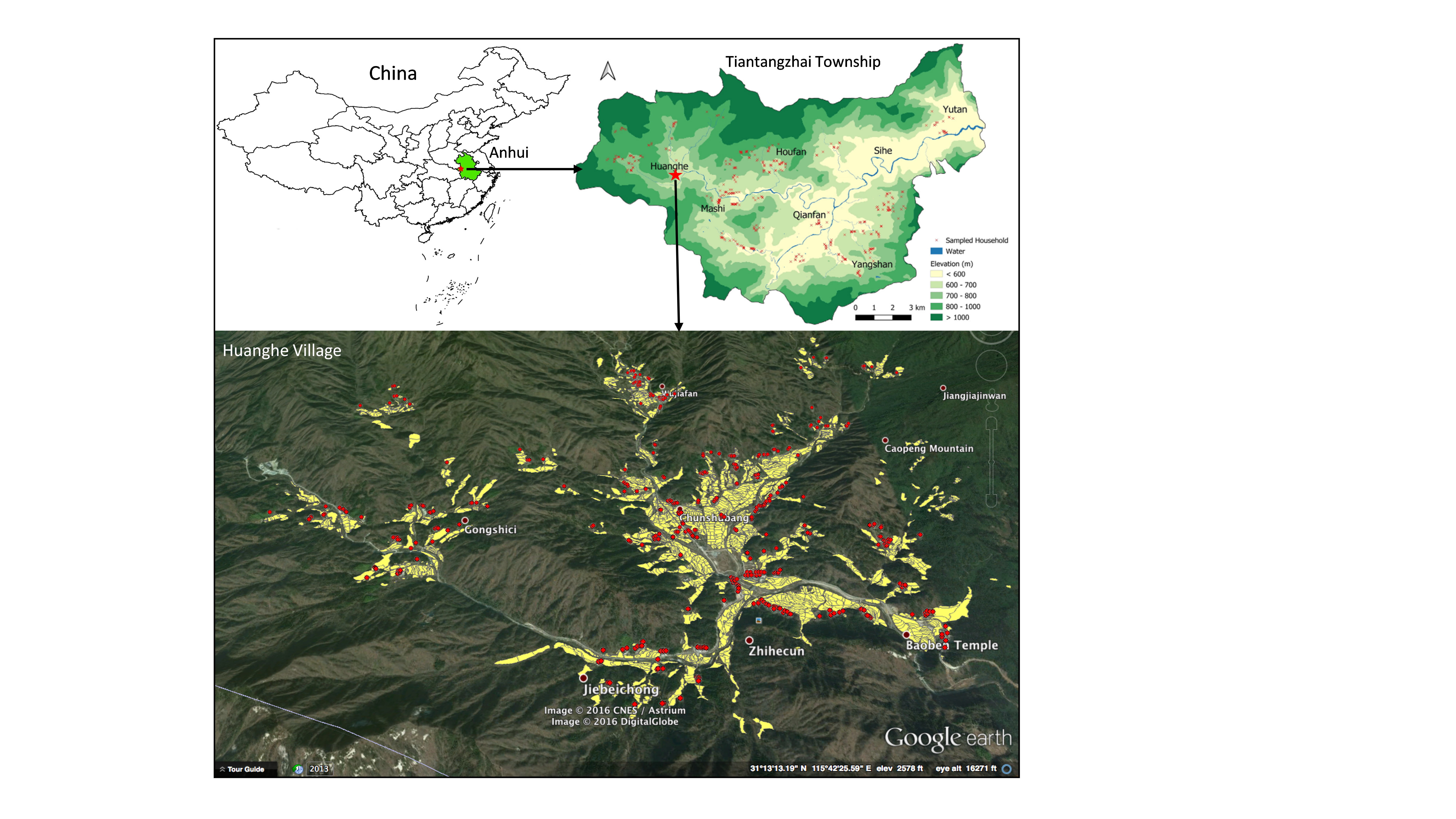
This study attempts to develop a spatially explicit ABM to explore households’ livelihood decision-making as influenced by agro-environmental policies in Tiantangzhai Township, Anhui province of China (Figure 1). The site under investigation locates in one of the 14 contiguous poverty-stricken areas of China that are designated as the main battlefields for poverty reduction going forward (Liu et al. 2005). As most of the contiguous poverty-stricken areas are ecologically important for ecosystem services (Zhou & Liu 2019), a number of agro-environmental programs with massive subsidies are implemented in these areas, including Tiantangzhai. Croplands in mountainous areas are often highly fragmented and situate in steep slopes with low productivity. Hence, households have to diversify income sources to secure livelihoods, which would further affect their cropland use. In this study, we are interested in studying livelihood decisions of individual labor engagements (i.e., on-farm work, local off-farm work, and labor migration) and household land allocation decisions (i.e., renting in, stabilization, shrinkage through renting out or abandonment). We also explore how the CNH systems evolve under two contrasting human behavior rules, i.e., the bounded rationality (BR) and empirical knowledge (EK), as affected by the agro-environmental policies. Understanding how rural farmers make labor and land allocation decisions in response to agro-environmental policies in Tiantangzhai Township can provide insights for the design of more effective policies in other contiguous poverty-stricken regions as well.
Methodology
Conceptual framework
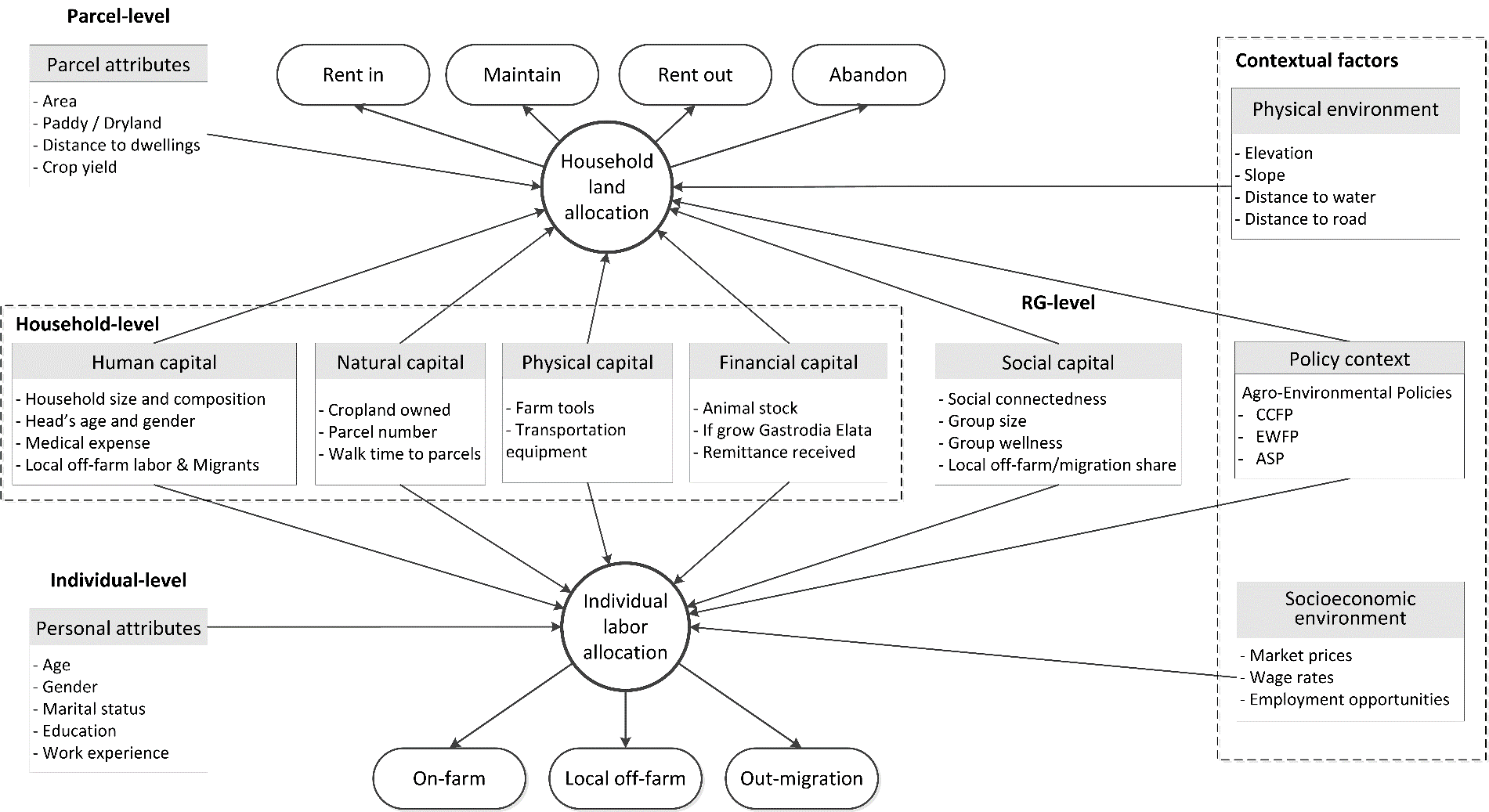
The conceptual framework of this study is presented in Figure 2. The overall objective of this study is to understand land and labor allocation decisions of rural households and their interactions with the landscape under agro-environmental policies. Regarding land allocation, we are interested in household’s cropland use decisions about whether to expand, stabilize, or shrink the cropland area, and whether to abandon or rent out land if the shrinkage decision is adopted. For labor allocation, we examine whether an individual chooses on-farm work, local off-farm work (paid work and business), or out-migration.1 According to the Sustainable Livelihoods Framework (DFID 1999), factors that may affect rural livelihood decisions include individual and household characteristics, household capital assets, policy intervention, and other contextual factors. Thus, for household labor allocation, we identify household-level factors that represent human, physical, natural and financial capitals, Resident Group (RG) level factors that measure social capital (e.g., group size and wellness) and environmental/geographic factors (e.g., elevation and distance to water). Additionally, attributes of each cropland parcel managed by a household, such as area, land type (paddy or dryland), distance to dwellings, and crop yield also influence the household land use decision-making. For example, households tend to rent out or abandon their marginal parcels that are small and located in remote area (Zhang, Song, et al. 2018). Generally, an individual’s labor allocation decision is determined by not only personal attributes (e.g., age, gender, and education), but also household capitals, social capitals in RGs, and local socioeconomic conditions (e.g., employment opportunities and wage rates). Moreover, both household land allocation and individual labor allocation decisions can be affected by different policies, including the CCFP, EWFP and the ASP (Wang et al. 2019, 2020).
Moreover, there exist feedbacks between household decisions and the influential factors. For example, a household may update its capital assets using economic returns from labor and land allocation activities; the social networks of a RG would change if more people engage in non-farm work; out-migration of household members will change a household’s member size and composition; the landscape would be altered following households’ land use decisions. These changes may serve as an important feedback impacting future decisions of rural households.
Development of ABM-LLA
We develop an empirical, spatially-explicit agent-based model to examine land and labor allocation (ABM-LLA) decisions of residents and households in a rural township in China. The model is comprised of social agents, landscape agents, and several key modules that define specific rules guiding how social agents behave and interact with other social agents and/or the landscape agents. Many complex features of human behaviors, such as sensing, interaction, learning and adaption, objectives, feedback, stochasticity, and emergence, are taken into account in model design (Table 1). The simulation starts at the year of 2013 when our household survey data was collected. Each simulation proceeds in an annual time step to simulate the real-world decision-making behaviors of social agents. The simulation runs for 18 time-steps, beginning from 2013 to 2030. The spatial extent of the model is the exact locations of all households and their cropland parcels. The ABM-LLA was coded and executed in NetLogo V6.0.4 (Wilensky 1999). Multi-dimensional data, including household survey data, field data geographically referenced with GPS, remotely-sensed images, and public statistics, have been collected and processed to parameterize the model. In this part, we will give an overview of the main structure and key modules of the ABM-LLA. A detailed description of the model following the ODD (Overview, Design of key terms, and Detailed information) protocol (Grimm et al. 2006, 2010) is provided in Appendix 1. The ODD protocol is a widely accepted guideline for describing ABMs, and is increasingly adopted by the social-ecological research community (Yamashita & Hoshino 2018; Zvoleff & An 2014).
| Concepts | Description |
|---|---|
| Sensing | 1. Individuals and households are aware of their own attributes (e.g., education and number of labor) and have perfect knowledge of the landscape characteristics, on which they make labor allocation and land use decisions are based.
2. Households have limited access to information of other households within same resident groups, such as available land to rent in, number of migrants, and number of off-farm workers. 3. Households can sense the socio-economic, geographic conditions, and policy interventions. |
| Interaction | 1. Social agents interact with the environment: households modify landscape via changing land use.
2. Social agents interact with each other: households in the same resident group can rent in/out cropland from/to others. During the farming season, households may hire other farmers to assist crop seeding, irrigation, and harvesting. |
| Objectives | ABM-LLA assumes that social agents are bounded-rational 1. At the household level, the basic goal of household livelihoods is to better allocate its most important household capitals, i.e., labor and land, to purse its livelihood goals of increasing household income. 2. At the individual level, each working age adult makes labor allocation decisions to maximize the expected economic return from employment conditioned by household livelihood capitals. An ordered-choice algorithm is adopted to seek an occupation that provides the highest income, but the employment probability is also considered, which represents the ability of individuals to be hired. |
| Learning/Adaptation |
1. When making labor allocation decisions, individuals can learn from their own work experience, and adjust their work to seek a higher economic return.
2. Households’ labor and land allocations are affected by their neighbors and other households in their resident group, e.g., if more households send family members to off-farm work or migratory work, they tend to increase labor inputs in these works as well. 3. Households adapt to the current socioeconomic environment (such as products market prices and wages), geographic conditions, and the policies to make more informed land use decisions. |
| Heterogeneity | The ABM-LLA model focuses on the micro-level behaviors of human agents, including simulation of each individual’s life history (i.e., birth, education, marriage, fertility, migration, and mortality) and labor allocation, and also households’ land use decisions, which manifest the feature of heterogeneity. |
| Feedback |
1. A household may update its capital assets (e.g., farm tools, transportation equipment) using economic returns from labor and land allocation activities.
2. The social networks of a resident group would change if more people living in the community adopt non-farm work. 3. Out-migration of household members may change a household’s size and composition. 4. The landscape would be altered following households’ land use decisions. The changes in an individual’s age and education, capital assets and demographics of households, social networks of resident groups, and the landscape would further affect individual and household decision-making. . |
| Stochasticity |
1. The values of some state variables of household and individuals are randomly generated based on statistical distributions derived from household survey data.
2. The probabilistic approach that integrates empirical knowledge and uncertainty is used to parameterize the behavior rules. The approach compares a random number with the probability of adopting a decision to determine whether the decision is made. This allows the simulation of stochasticity. |
| Emergence |
1. The human agent’s population dynamics at an aggregated level emerge from the behavior of each individual and household following a bottom-up process.
2. The landscape dynamics at the regional level (e.g., the shares of cultivated land and abandoned land) emerge from each farming household’s land use decisions. 3. The use of fertilizers and pesticides by farming households at the household level may bring environment pollution to larger areas as the agricultural pollutants in the soil may reach far with the stream flow. 4. Livelihood performance of the entire household at the household level (e.g., increased household income and decreased poverty) emerges from each individual’s labor allocation behaviors at the individual level |
Agents and state variables
There are two types of agents in the ABM-LLA: social agents, i.e., social individuals that actively make decisions; and landscape agents, i.e., passive entities that are owned, managed or manipulated by human agents.
Social agents are further divided into individuals, households and RGs. Individual agents represent living rural residents, each of which is characterized by a set of state variables, including unique identification number (ID), household-ID, age, gender, lifecycle stage, marital status, work status, and annual income. The major life choices and events of an individual, including birth, education, jobs and income, marriage, fertility, migration, aging and death, are taken into account in model design (Figure 10 in Appendix 1). Household agents are formed by individuals with the same household-ID, with state variables of household-ID, ID of the RG in which it resides, household size and composition, livelihood capitals (e.g., cropland owned, farm tools, transportation equipment), and policy engagement (participation in agro-environmental policies and payments received). Households are spatially distributed in the study area based on their geographic locations. Major behaviors of household agents include land allocation decisions and update of household sizes and livelihood capital assets. RG agents are local collective-management communities that are composed of households residing geographically close to each other with the same RG-ID. Major events of RG agents involve updating group size, mean wellness and percentages of households involved in off-farm and labor migration. Changes in general wellness and employment status of a RG would affect decisions of residents and households residing in it.
Landscape agents are categorized into two types, i.e., environmental grids and cropland parcels. Environmental grids are raster grids that constitute the biophysical environment where social agents situate, interact and make decisions. State variables of each environmental patch include slope, elevation, its distance to nearest river and paved road. These attributes are considered as stable during our simulation. Cropland parcels are represented in vector polygons, which are delineated in ArcGIS based on field survey and imported into NetLogo. Each parcel is linked to its household owner through a parcel use right owner ID. Other state variables include parcel area, parcel type (i.e., paddy-land or dry-land), distance to dwellings, land use status (i.e., stabilized, rented in, rented out, or abandoned), and parcel yield.
The descriptive statistics and data sources for key parameters of the four types of agents in the ABM-LLA are reported in Table 2.
| Agent type | Key parameters | Description | Unit | Mean | Std. Dev. | Data source |
|---|---|---|---|---|---|---|
| Individual agents | Age | In years | years | 40.5 | 20.0 | Census and household survey data |
| Gender | 1=male; 0=female | % | 56.0 | 49.6 | ||
| Education | Years of schooling | years | 5.4 | 3.7 | ||
| Marital status | 1=married; 0=never married, divorced or widowed | % | 71.3 | 45.3 | ||
| Household agents | CCFP participation | 1 = yes; 0 = no | % | 56.5 | 49.6 | Census and household survey data |
| EWFP subsidy | Subsidies from EWFP | yuan | 592.4 | 667.4 | ||
| ASP subsidy | Subsidies from ASP | yuan | 695.8 | 1340.1 | ||
| Household size | Number of household members | persons | 2.9 | 1.3 | ||
| Education of head | Education of household head | years | 5.9 | 3 | ||
| Local off-farm labor | Number of household members engaged in local off-farm work | persons | 0.5 | 0.7 | ||
| Medical expense | Household annual expenditures on medicines and health care in past 12 months | yuan | 4077.6 | 7028.7 | ||
| Migrants | If has former member(s) working in non-local labor market | % | 66.2 | 47.4 | ||
| Cropland owned | Area of cropland owned | mu | 5.7 | 2.7 | ||
| Parcel number | Number of cropland plots endowed | count | 3.5 | 1.8 | ||
| Walk time (plots) | Mean walk distance to cropland plots | minutes | 11.1 | 8.2 | ||
| Farm tools | Score of farm tools, see Appendix 2 | index | 2.5 | 1.6 | ||
| Transportation equipment | Score of transportation equipment, see Appendix 2 | index | 2.5 | 1.4 | ||
| Animal stock | Value of animals | yuan | 4519.2 | 8774.8 | ||
| If grow Gastrodia Elata | 1 = yes; 0 = no | % | 57.6 | 49.5 | ||
| Remittance received | Amount of money received by household from migrants | yuan | 9998.1 | 20287.6 | ||
| Social connectedness | Sum of money sent and received as social gifts/total annual income | % | 47.0 | 79.4 | ||
| Resident group agents | Group size | Number of households in the resident group a household belongs to | households | 26.1 | 8.6 | Census and household survey data |
| Group wellness | Mean household wellness index in resident group | index | 20.2 | 2.1 | ||
| Environmental patches | Slope | Slope of the patch | degree | 17.4 | 7.9 | Landsat images and DEM |
| Elevation | Elevation of the patch | meters | 955 | 195 | ||
| Distance to river | Distance of the patch to the nearest river | meters | 732 | 622 | ||
| Distance to road | Distance of the patch to the nearest paved road | meters | 577 | 493 | ||
| Cropland parcels | Parcel area | Area of the parcel | mu | 1.8 | 1.8 | Worldview-2 image and the land titling map |
| Parcel type | 1 = paddy; 0 = dryland | % | 85.0 | 35.7 | ||
| Distance to dwellings | Distance from the parcel to the house of its owner | meters | 397.2 | 339.1 | ||
Process overview
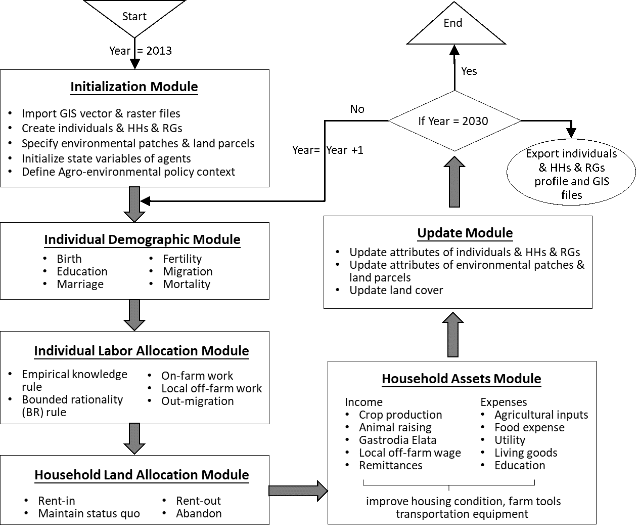
The conceptual framework of ABM-LLA (Figure 2) was implemented in six major modules: Initialization Module, Individual Demographic Module, Individual Labor Allocation Module, Household Land Allocation Module, Household Assets Module, and Update Module. The model begins with the Initialization Module to create the landscape, import environment layers and cropland parcels, generating individuals, households and RGs, and set up initial states for different types of agents. This module is executed only once at the beginning of the model simulation, while the other five modules are repeated in each time-step successively to simulate the decision-making processes of social agents and dynamics in the CHN systems until the model stops at the end year of 2030. Figure 3 illustrates the major modules and the linkages among them that reflect feedbacks.
First, the Individual Demographic Module is executed to simulate each individual’s life history, including birth, education, marriage, fertility, migration, and mortality. After this module, all individuals are categorized into four age groups: preschool age (0–6 years), school age (7–15 years), working age (16–64 years), and elderly age (65+ years).
Then the Individual Labor Allocation Module is implemented for individuals in working age to simulate their allocation of their labor time to competing livelihood activities, i.e., on-farm work, local off-farm work, and migratory work. Here, we use two different rules to parameterize individual labor allocation decision, i.e., the empirical knowledge (EK) and bounded rationality (BR). The EK rule relies on empirical knowledge gained from household survey data and implemented with empirical models. We use the binary logistic regression to predict the probability for an individual to adopt local off-farm or migratory work based on a host of factors, including personal attributes, five dimensions of livelihood capitals and the policy context (i.e., CCFP and EWFP participations, ASP subsidies). The estimated coefficients for the regression model are listed in Table 3. Then the probabilistic approach is adopted to determine whether an individual adopt local off-farm or out-migration. The approach draws a random number in [0,1] and compares it with the estimated probability, if the number is smaller than the portability, then the specific decision would be taken. If both decisions are not adopted, the person would prefer on-farm work.
| Variables | Migration Base = On farm |
Local off-farm Base = On farm |
|||||
| Coeff. | S.E. | \(p > z\) | Coeff. | S.E. | \(p > z\) | ||
| Personal condition | Gender | 1.346 | 1.151 | 0.000*** | 3.817 | 34.024 | 0.000*** |
| Marital status | 0.932 | 1.327 | 0.075* | 0.698 | 1.540 | 0.363 | |
| Age | -2.306 | 0.024 | 0.000*** | -2.275 | 0.047 | 0.000*** | |
| Education | 0.025 | 0.143 | 0.857 | 0.607 | 0.624 | 0.074* | |
| Policy context | CCFP participation | 0.610 | 0.386 | 0.004*** | 0.214 | 0.474 | 0.576 |
| EWFP subsidy | -0.094 | 0.133 | 0.522 | 0.439 | 0.384 | 0.077* | |
| ASP subsidy | 0.196 | 0.139 | 0.086* | -0.195 | 0.148 | 0.278 | |
| Human capital | Household size | -0.640 | 0.091 | 0.000*** | -1.897 | 0.061 | 0.000*** |
| Local off- farm labor | -0.396 | 0.109 | 0.014** | -0.024 | 0.297 | 0.938 | |
| Medical expense | 0.026 | 0.156 | 0.863 | 3.969 | 31.852 | 0.000*** | |
| Migrants | 0.149 | 0.633 | 0.785 | ||||
| Natural capital | Cropland owned | -0.038 | 0.142 | 0.795 | 0.325 | 0.376 | 0.232 |
| Parcel number | -0.125 | 0.129 | 0.393 | -0.818 | 0.101 | 0.000*** | |
| Walk time (parcel) | -0.131 | 0.109 | 0.292 | -0.321 | 0.169 | 0.168 | |
| Physical capital | Farm tools | 0.240 | 0.165 | 0.065* | -0.010 | 0.247 | 0.969 |
| Transportation equipment | -0.168 | 0.127 | 0.263 | -0.539 | 0.179 | 0.079* | |
| Financial capital | Animal stock | -0.446 | 0.178 | 0.108 | 0.016 | 0.267 | 0.950 |
| If grow Gastrodia Elata | -0.171 | 0.119 | 0.228 | -0.721 | 0.273 | 0.199 | |
| Remittance received | 0.368 | 0.216 | 0.014** | 0.222 | 0.287 | 0.336 | |
| Social capital | Social connectedness | -0.111 | 0.124 | 0.424 | 0.308 | 0.299 | 0.163 |
| Group size | 0.139 | 0.161 | 0.322 | 0.1 | 0.345 | 0.621 | |
| Group wellness | 0.311 | 0.175 | 0.016** | 0.072 | 0.338 | 0.819 | |
| Constant | -1.93 | 0.077 | 0.000*** | -4.821 | 0.008 | 0.000*** | |
| Model summary | Wald \(Chi^{2}\)= 179.81, \(p < 0.001\) Log-pseudo likelihood = -4897.85 Pseudo \(R^{2}\) = 0.43 |
Wald \(Chi^{2}\)= 111.90, \(p < 0.001\) Log-pseudo likelihood = -1347.79 Pseudo \(R^{2}\) = 0.70 |
|||||
The BR rule assumes individuals can use their limited information, experiences, and resources to make a perceived optimal choice. Under the BR rule, an individual estimates economic returns from the three types of work (on-farm, local off-farm, and out-migration) based on its own experience and that of its neighbors. Specifically, if an individual is a new labor who has just joined the labor force, he/she would make the labor allocation choice based on information gathered from neighbors. We assume that the individual would search three other labor individuals at neighboring households, acquires information of their incomes for all possible livelihood activities including on-farm work, local off-farm work, remittances from out-migrants, and compare their incomes to select the job with the highest income. To account for the randomness and the ability of an individual to be hired, the probabilistic approach is further adopted to decide whether an individual can eventually engage in the preferred work. Meanwhile, for an individual already involved in one type of work, his/her decision is whether to change a job that would bring higher income. The individual searches three other neighboring individuals engaged in the other two types of work and would change his/her work if the highest neighboring individuals’ income is higher than the current income of the given person.
Afterwards, the Household Land Allocation Module is executed for households that have cropland parcels and available farm labor to simulate their land use decisions about whether to expand (rent in), maintain status quo or shrink cultivated cropland area (rent out or abandon) during each time-step. We first use a multinomial logistic model to predict the probability for a household to adopt stabilization, expansion or shrinkage based on a wide range of factors including policy context and five forms of capital, i.e., human, social, physical, natural and financial; and then apply a binary logistic model to predict whether renting out or abandonment is preferred if the decision of cropland shrinkage is adopted. The selection of explanatory variables and estimation of parameters are introduced in greater detail in Wang et al. (2019). The estimated coefficients are also shown in Tables 8 and 9 in Appendix 1. The land allocation decisions would change the land use status of cropland parcels.
Thereafter, the Household Assets Module calculates a household’s incomes derived from agricultural production, non-farm work, remittances from migrants, and governmental subsidies; and costs of agricultural inputs, living costs, education expense, medical expense, etc. Specifically, the Cobb-Douglas production function is applied to estimate yields of crops based on a variety of agricultural inputs (e.g., agricultural labor, cropland area, expenses of fertilizers, pesticide, seeds, and hired labor) and the age and education of household’s head.
At the end of each time step, the Update Module would be applied to update state variables of all agents. Notably, the changes in an individual’s age and education, capital assets and demographics of households, social networks of resident groups, and cropland use would further affect individual and household decision-making. This allows the simulation of multiple feedbacks occurring at different levels within the CHN systems over time. Finally, results of interest including dynamics in human and land systems will be generated during each simulation.
Model verification and validation
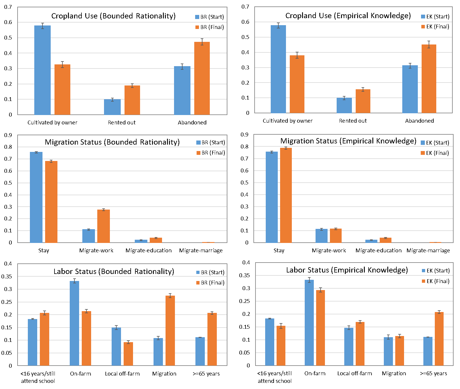
We adopt the verification and validation protocol proposed by An et al. (2005) to verify and validate the ABM-LLA, involving model debugging, uncertainty testing, empirical validation, and sensitivity analysis. During the process of extreme value tests, the model was corrupted at some stages or returned unreasonable outcomes. We carefully examined the codes and conducted uncertainty tests repeatedly until no model corruption occurs. Empirical validation is conducted by comparing the initial value distributions of state variables of human and landscape agents generated by the initialization module of the ABM-LLA with the descriptive statistics of household survey data. In addition, we plotted the distributions of initialized land and labor allocation status and simulated outputs after the model simulation, including cropland use, migration status and labor status for both BR and EK rules. Results show the distributions generally fit well and reflects what was expected (e.g., cropland shrink and higher migration likelihood under the BR rule), which demonstrates that the module of initialization and simulation can represent the human agents and the landscape of the real-world (Figure 4). Since stochasticity is a main feature of the ABM, it is difficult to conclude from one single simulation. In this study, we conducted independent simulations for 50 times, and derived the means of the outputs and their standard deviations. This is an effective way to quantify the model outputs and its uncertainty (Le et al. 2010). Finally, sensitivity analysis was conducted to test the model robustness to changes of input parameters. Sensitivity can be assessed by perturbing each major parameter and then analyzing the variations in model outputs, such as the results shown in policy experiments.
Policy experiments
We designed four policy-related scenarios regarding the three programs, namely CCFP (2 scenarios), EWFP (1 scenario) and ASP (1 scenario). Under all the scenarios, we performed the model experiment for the two behavior rule settings, i.e., BR and EK. This constitutes a total of 8 scenarios for model experiments so as to provide a comprehensive understanding of the complexity regarding the policy effects. Below we describe the detailed design of the policy scenarios.
- In our study site, only a small proportion participated CCFP by enrolling some cropland parcels for reforestation. This allows us to create sample households with some participating into CCFP while others not. Accordingly, in the model, we divided the household into two groups, CCFP participating households and nonparticipants. The first scenario is focused on the outcomes (see below) by comparing the participating household group and the nonparticipating group. The lasting period is assumed to cover the whole modeling process, i.e., 18 years.
- The second scenario is still related to CCFP but focused on how long did CCFP last for providing subsidies to participating households. Here, we set three cases in which CCFP terminates after 5, 10, 15 years of providing subsidies since the start of the model. We then compare the outcomes under the three cases of termination years.
- In the third scenario design, we aimed to test the EWFP effects. One issue is that nearly all households manage some EWFP forests and hence automatically participate in the EWFP program. Thus, there are almost no nonparticipants for comparison. In this case, we divided the households into two groups based on how much subsidies they receive from EWFP, specifically the above-mean groups and below-mean group representing households receiving subsidies above and below the mean amount of EWFP subsidies of all households. This allows us to compare outcomes for households who receive more EWFP subsidies in contrast to those receiving less.
- The last scenario design is similar to that for EWFP, but focusing on ASP. As almost all households receive a certain amount of subsidies from ASP. We divided the households into above-mean and below-mean groups for the comparison.
We assessed the policy impacts on the outcomes in terms of a variety of indicators, including i) total population and per capita income, ii) mean percentage of household labor allocated to agricultural production, local off-farm work and migratory work, respectively, and iii) land allocation, including mean percentage of households adopt expansion, stabilization, renting-out, and abandonment, respectively. These indicators are computed at the village level.
Results and Discussion
Labor and land allocation under bounded rationality (BR) vs. empirical knowledge (EK) rules
We observe substantial differences of outcomes between the BR and EK rules over the simulation period of 2013-2030, as shown in Figure 5. In terms of socioeconomic outcomes, total population of local residents in Huanghe Village slightly increases under the EK rule. However, it falls sharply following the initialization year and then gradually decreases under the BR rule. This is because that, under the BR rule, an increasing number of residents migrate out to seek better opportunities, as income from work in cities is higher and increases at a faster rate than the other sources. In contrast, a growing number of individuals engage in local off-farm work under the EK rule. Regarding the mean per capita income, people are expected to earn more under the BR rule than EK rule, and the gap widens over time. In addition, labor time allocated to on-farm work declines under both rule settings, suggesting a continued trend of farmers quitting agriculture. This is expected because of the limited economic return from agricultural production, which, however, may pose great threat to food security in the long term.
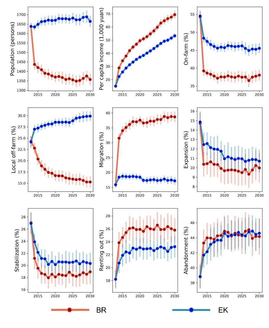
In terms of land allocation, a growing number of households shrink cultivated cropland under both rule settings, either via abandonment or renting-out. Compared to the EK rule, the percentage of households renting land out under the BR is higher. As more people migrate to cities and people follow the “rational” rule to maximize economic return from all sources under the BR rule, households are more inclined to lease cropland for rents, instead of abandonment. In contrast, the share of households expanding or maintaining croplands is larger under the EK rule than the BR rule. Under the EK rule, individuals tend to seek non-agricultural jobs or businesses in relatively short distance from their households so they could help with farm work when necessary.
Spatial patterns of land allocation decisions
Based on the geolocations of cropland parcels, we are able to map the spatial patterns of changes in multiple land use decisions (Figure 6). We first divide the cropland parcels into three groups based on the land use status, including parcels planted by owners, planted by others (rented out), and abandoned. For each parcel in each year, we calculate the proportion of the number of model runs with the occurrence of each status in the total number of model runs as the likelihood of the given land use status. Then, we take the absolute difference of the proportions in the final year (2030) and the first year (2013) as the value to represent the changes in status of cropland parcels. We also plot the distributions of three status changes for the 2,225 parcels (Figure 11 in Appendix 3).
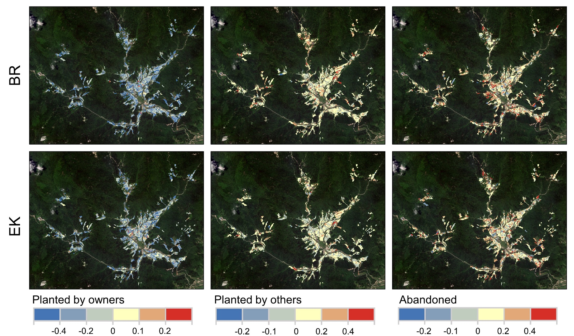
Under both rule settings, there is a decreasing trend of the likelihoods for parcels to be planted by owners, while the parcels tend to be either rented out or abandoned. In terms of the latter two cases, the extent to which parcels are abandoned is slightly higher than that of being rented out. This is evident that there are more parcels with larger positive changes (depicted in orange or red) in likelihood of being abandoned. Notably, there is a hot spot of cropland abandonment in the middle west of the main residential area, where parcels are likely to be small in area and located in high elevations. Meanwhile, a hot spot of renting-out/in parcels is found to be along the main roads in the northeast of the main residential area. In this place, parcels have relatively large in areas with decent quality and easy access. Thus, households who allocate labor for off-farm activities may tend to raise income by renting out these parcels other than entirely abandoning them.
Moreover, under the BR rule, cropland parcels, particularly those located in high elevations and/or remote areas, are more likely to forgo land cultivation as more parcels are identified with greater negative changes (depicted in darker blue) than the EK rule. For renting-out and abandonment, the overall patterns are similar under the two rules, but the BR rule shows more parcels with greater positive changes in either renting-out or abandonment of parcels. Overall, these results reflect that, over the study period, most households are less likely to plant their own cropland parcels while renting out or abandoning parcels (preferred) in remote areas with poor accessibility.
Impacts of Agro-environmental Policies: Impacts of CCFP
The effects of the CCFP on household labor and land use decisions are substantial, with noticeable differences before and after CCFP terminates, and between households participating and not participating the program (Figure 7). The payment of CCFP is set to terminate by 2020 according to the actual policy design (State Forestry Administration 2015).
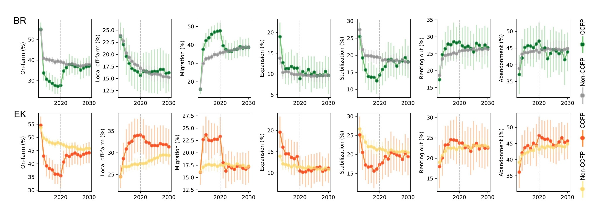
First, CCFP has a positive impact on migratory work, and the impact tends to decrease when CCFP ends in 2020. In contrast, CCFP tends to demotivate agricultural production, as a declining trend of on-farm labor allocation is observed among CCFP participants under either BR or EK rule. CCFP participation requires the household to retire cropland, creating a labor surplus for migratory labor markets. Previous studies in various regions also suggest that CCFP has promoted out-migration (Démurger & Wan 2012; Uchida et al. 2009; Zhang, Bilsborrow, et al. 2018). The largest difference between the two behavior rules is for local off-farm employment. Under the BR rule, the local off-farm employment for both groups fall, with CCFP participants decreasing faster than non-participants before 2020. As remittances from migrants may provide a larger amount of income, households tend to adopt this activity to maximize total income. However, under the EK rule, CCFP households also shift the surplus labor to local off-farm work and have higher change to diversify their livelihoods.
As for land allocation, CCFP has positive impacts on cropland shrinkage, but is negatively linked to stabilization or expansion. Under both rule settings, the share of households adopting the renting out or abandonment decision increases faster among participants than non-participants before 2020. After CCFP terminates, the probability of renting-out or abandonment does not show a particular trend over time. Under the BR rule, CCFP participants prefer renting land out to abandoning land, comparing to non-participants, given households are able to make “rational” decisions. The EK rule displays a different picture, with participants continuing to have larger abandonment shares than non-participants even after CCFP payment ends. Moreover, CCFP seems to encourage its participants to rent in some cropland to replace the land set aside for reforestation, as the expansion share for CCFP participants is larger than that of non-participants, especially under the EK rule.
To explore how CCFP implementation years affect household decision-making, we assume households are notified that CCFP will end in 5, 10, and 15 years, respectively, and observe the performance indicators (Figure 12 in Appendix 3). Note that only CCFP participants are included in this experiment. Under the EK rule, individuals tend to stay on-farm when CCFP is expected to end in 10 years, but choose local off-farm work when CCFP ends in 5 years. Under the BR rule, the local off-farm share is relatively large when CCFP ends in 5 or 10 years than in 15 years. Overall, impacts of CCFP implementation years on household land use decisions are complicated and non-linear.
Impacts of EWFP
As nearly all households receive EWFP subsidies, we separate the households into two groups by EWFP payment amounts, including those receiving above-mean payments and below-mean payments. There exist relatively great discrepancies regarding labor and land allocation between the two groups (Figure 8).
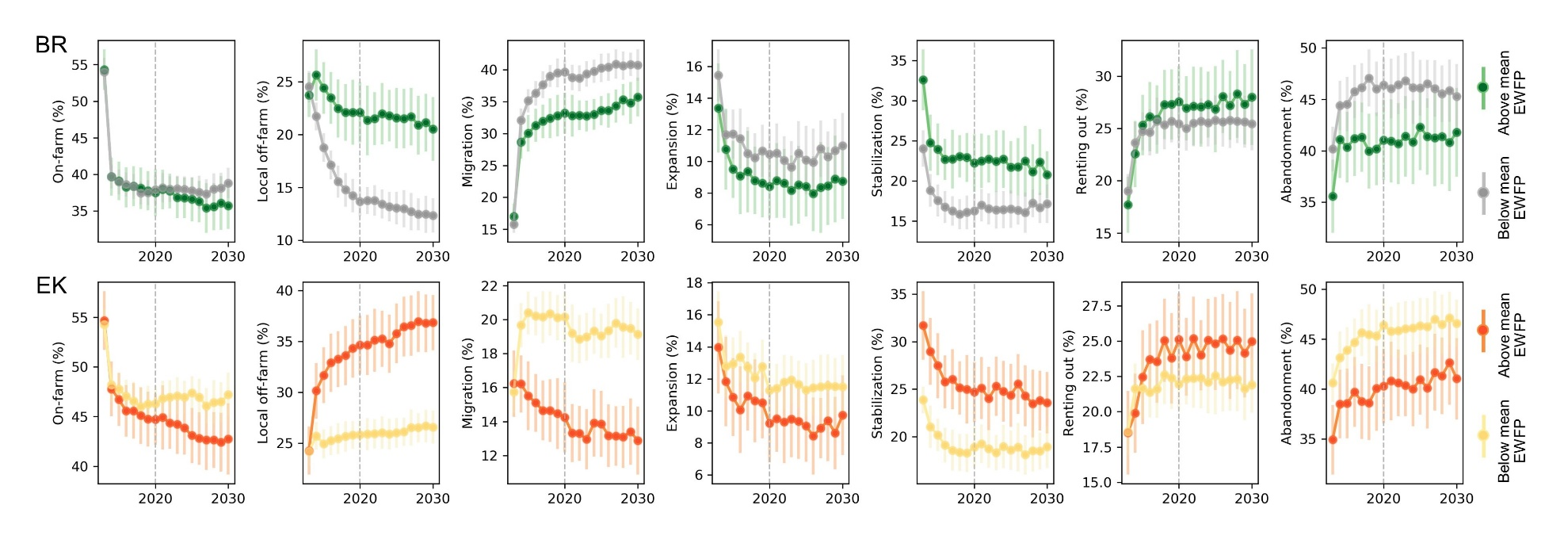
Under both rule settings, households with relatively more EWFP payments allocate much more labor time to local off-farm jobs, while those with below-mean EWFP payments have much higher probability to migrate to work in cities and slightly larger possibility to work on-farm. Households receiving higher payments often reside in higher elevations with poorer transportation linkages since they manage larger areas of natural forests, namely ecological welfare forests (Dai et al. 2009). Residing in local areas allows them to diversify livelihoods by growing Gastrodia Elata, as they have easier access to natural forests. In contrast, households receiving fewer EWFP payments usually live at lower elevations with more social, human, and financial capitals, which make them easier to send migrants to cities (Poot et al. 2009). The BR rule reveals a gradual shift among labor allocation activities from on-farm and local off-farm to migratory work over time, with those that receive below-mean EWFP payments changing at a faster rate. In contrast, different change trends can be seen between the two groups under the EK rule.
Changing trends of land allocation are similar under the two rule settings. In particular, EWFP payments tend to positively affect stabilization or renting out, as the above-mean EWFP group has higher shares of households adopt these two decisions than the below-mean group. This could be because that higher EWFP subsidies enable the households to reduce the burden of land cultivation, and more inclined to rent land out for less income. Moreover, more households from the below-mean group expand cropland than the above-mean group, but the percentage follows a downward trend for both groups. In contrast, the abandonment exhibits an upward trend, agreeing with a previous empirical research in the same study area (Zhang et al. 2018).
Impact of ASP
We compare social-ecological outcomes of ASP between the above- and below-mean subsidy groups. Results suggest that most of the activities on labor and land allocation are substantially different between the two ASP based household groups for both rules setting (Figure 9).
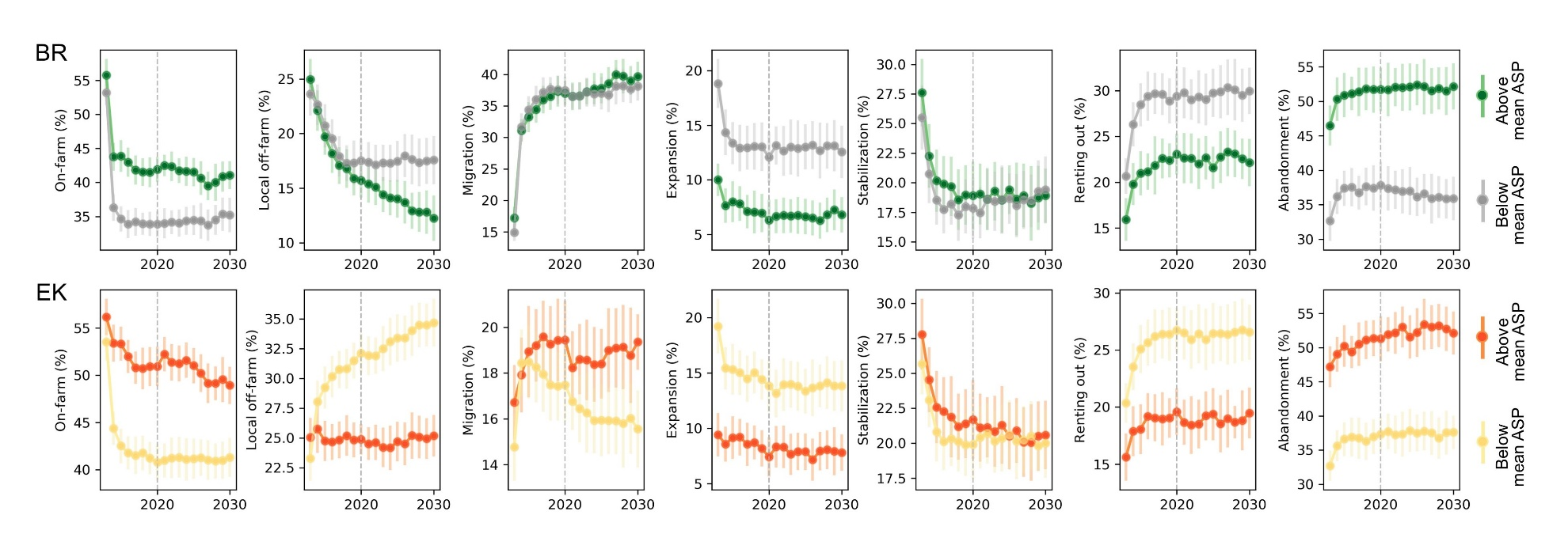
Regarding socioeconomic performances, under both rules, there are more individuals from the above-mean ASP group choosing to work on-farm than the below-mean group. This suggests that the agricultural subsidies are effective in stimulating rural farmers to continue agricultural production, in line with the policy goal instrument (Guo et al. 2019; Huang & Yang 2017; Liu et al. 2005). However, this incentive effect dissipates over time, as labor time is gradually shifted to migratory work (under BR-rule) or local off-farm work (under EK rule). Under the BR rule, the rapid decrease of local off-farm share was exhibited until the fifth year for those with below-mean subsidies, while the downward trend continues throughout the simulation period for the above-mean subsidy recipients. Both groups show similar growing trends of the migration decision. By contrast, under the ER rule, the local off-farm adoption for the below-mean group increases steadily, but remains stable for the above-mean group. Moreover, the below-mean group undergoes a steady decline in migration after year two, whereas the migration percentage for the above-mean group fluctuates at a relative higher value.
The predicted trends for different land allocation decisions under the BR and EK rules are generally similar. Surprisingly, increases of the agricultural subsidies result in significant higher shares of abandonment, and slightly higher portions of stabilization, which is contrary to policy expectations. This might be attributed to the weakness of the program in precisely targeting the households that actually cultivate land. In most areas, ASP subsidies are still given directly to cropland use right owners, rather than the farmers produce agricultural outputs, like many other rural areas in China (Huang et al. 2011), thus not effective encouraging farmers to keep land under cultivation. Another reason is that households receiving higher ASP subsidies often possess more cropland parcels and live in more rugged terrain area. Some of the parcels are inevitably of marginalized quality. It seems ASP tends to keep more households employed for the good quality cropland, but does not prevent the abandonment of cropland with marginalized quality. In contrast, households with below-mean ASP subsidies show greater inclinations towards expansion or renting out than the above-mean group. A possible explanation is that households with lower ASP subsidies possess less land resource. Thus, they are in greater need to expand cropland when on-farm employment is pursued, and value the land more than those with larger land areas, leading to preference of renting out land instead of abandoning it when they decide to cultivate less cropland.
Implications and Future Work
Policy implications
Policy implications for forest conservation and agricultural stabilization can be drawn from our findings. China’s large-scale rural-urban out-migration generates great needs to rent land out or abandon cropland. However, as rural areas in China often have low in-migration or return-migration rates, and rural youths are unwilling to engage in farming (Liu et al. 2016), the population of farmers are decreasing and aging, which is especially true in mountainous areas. Who cultivates the cropland to maintain food production level becomes a critical issue faced by China (Khan et al. 2009; Ye et al. 2013). To promote sustainable development of agriculture, significant reforms need to be made to current agricultural and land use policies. First, the agricultural subsidies should be provided to actual cultivators while land fallowed or abandoned might not be provided with agricultural subsidies. Second, it is crucial to increase the number of “professional farmers” (Yang 2013), who are young or middle-aged, well-educated, and are willing to practice modern agriculture or large-scale farming. Additional incentives, e.g., new agricultural technique trainings, could be provided to these farmers to promote agricultural development. Third, as more out-migrants settle down in urban areas, it is possible to introduce a cropland contractual right exit mechanism to encourage transfer of right from households to the rural collective (Su et al. 2020). The Chinese government is reforming the tenure system for land in rural areas, and enacting the “Three Rights Separation Policy” (TRSP) (Wang & Zhang 2017). While persisting the collective rural land ownership, the new policy separates farmers’ contract and management rights. This separation allows e.g. companies to manage the lands for farmers who are willing to transfer use rights (Xu et al. 2018). An interesting topic that extends the current research is to test the complex farmers’ decisions on land use and livelihoods under various environmental conditions such as climate change and extreme events (Entwisle et al. 2016). The environmental policies in China partially (or even more critically) result from frequent natural disasters, aiming to conserve water and soil for ecosystem services (Zhang et al. 2000). The interacting directions and magnitudes of farmers and the land may be shifted by these unexpected events that further influence the whole complex system (Walsh et al. 2013). Thus, an agent-based model incorporating more of the environmental elements would be useful for broadening the perspectives regarding policy implications.
ABMs often rely on social and economic theories on human behavior to understand the decisions which can be explored via rule-settings (An 2012; Elsawah et al. 2015). Two distinct designing rules follow practices with choices under rational thinking (BR) and with knowledge empirically acquired from existing information (EK). One of the major differences of modeling outputs between the BR and EK rule settings is that households under the BR rule make livelihood decisions based primarily on information gained from neighborhood social networks, while households’ livelihood strategies are made according to personal attributes and household capital under the EK rule. This suggests social networks may affect the impacting pathways and effectiveness of agro-environmental policies on rural household livelihoods (Entwisle et al. 1998; Hauck et al. 2016; Jiang et al. 2015; Morris 2004). For example, households enrolled in the CCFP reallocate the freed-up labor to local off-farm work or migrate to work in cities and receive higher economic return than that from agricultural production (Song et al. 2014). This shift in labor could raise the enrollment of the CCFP and change labor allocation choices of neighborhood households (Chen et al. 2009). Thus, social network effects can be used to optimize agro-environmental policies as the outcome of policy intervention may spread through socially connected households (Hauck et al. 2016). Policy instruments targeting the important nodes with large numbers of connections in a social network may improve the efficiency of policies. However, due to network propagation, undesired responses to policy invention made by those important households in social networks may dampen the effectiveness of polices. Thus, depicting within-village social networks, and investigating the interaction effects of policy instruments and social networks on household livelihood decisions are the focus of our future research.
ABM simulations
Relying upon multi-dimensional datasets including household survey data, census data, field survey data, statistical data from public reports, and remotely-sensed data, we develop an empirical agent-based model (i.e., ABM-LLA) focusing on the decision-making processes of social agents (including farmers, households and resident groups) and their interrelations with the environment (represented by landscape agents). The major demographic processes of individuals, such as education, marriage, fertility, labor allocation, migration and mortality are taken into consideration. Moreover, based on an officially verified land titling map with signatures of farmers, each household and its owned land parcels could be spatially linked. Thus, the model allows the spatially explicit representation of micro-level human behaviors in landscape change processes from a bottom-up perspective, and their interactions can be modeled in a direct way (Filatova et al. 2013; Kremmydas et al. 2018). The model serves as a laboratory to run multiple experiments under different parameter settings or combinations for testing the effects of different factors of interest, especially the agro-environmental policies.
There are caveats for ABM-LLA. Due to the lack of longitudinal survey data, we could only validate the model at the initialization stage using the household survey data collected in 2014 and 2015 as all these data were used for parameterization of the model, while subsequent simulations cannot be validated. The main purpose of the model in this research is to understand complex interactions between social agents (individuals, households, resident groups) and the environment (landscape) instead of making predictions. Thus, the focus here is testing outcomes under various policy scenarios and comparing the different decision-making rules including empirical knowledge and bounded rationality. It is also admitted that the future work of the model application includes better validation approaches with uncertainty fully addressed. Regarding spatial attributes, one promising way is to leverage satellite data that are independent of the currently used data to validate the spatial patterns, although a final spatial resolution is necessary. We will also conduct follow-up surveys to improve the validation and enhance the reliability of the model. Moreover, the macro-environmental conditions, such as changes in climate and global market, and local contextual factors, such as soil quality and irrigation, are assumed to be constant through time. Due to the small-scale area in the village, it is recognized that there is little variation in these contextual factors, exhibiting trivial influences to agents’ behavioral changes at the local level. Furthermore, the impacts of household livelihood decisions on ecosystems are not evaluated in the model. Such evaluating processes requires sophisticated components with ecological models monitoring biophysical processes, which is nevertheless not the focus in this study. Our future work will characterize the changes in the biophysical condition with time along with local manifestation of global climate change and market dynamics.
Conclusions
In this paper, we used an agent-based model with socioeconomic and spatial data in rural China (Tiantangzhai Township in Anhui Province) to study the impacts of three agro-environmental policies (i.e., CCFP, EWFP and ASP) on rural households’ labor and land allocation decisions. We applied two methods to design behavioral rules, one relying on empirical knowledge (EK) and the other bounded rationality (BR) and compare the outcomes between the two rules. The largest difference was that more households adopt local off-farm work under the EK rule, while more households send out migrants under the BR rule. Both scenarios exhibited decreasing likelihoods of on-farm employment and cropland expansion, but increasing inclinations to rent out or abandon cropland. It is desirable to develop rural land transfer markets and accelerate the reform of rural land tenure system to enhance land use efficiency. Meanwhile, CCFP participation has positive effects on labor out-migration with reduced cropland use. Effects of EWFP and ASP on household labor allocations vary largely under the two rules, but their impacts on land use decisions are similar. Overall, the impacts of the agro-environmental policies are non-linear and not fully conform to policy expectations, which are largely due to the complex interactions and feedbacks between rural households and the local environment. The agent-based model offers a way to investigate these interactions and unpack the complexity of CNH systems.
Notes
On-farm work refers to agricultural work, including crop cultivation, animal husbandry, forest resource management, and other agriculture-related activities. Local off-farm work refers to managing a local business (e.g., a restaurant, a convenience food store, providing a service) or employment in which a wage or salary is received from others. Out-migration refers to work outside the county for at least 6 months consecutively in a year.↩︎
Acknowledgements
This research was supported by the National Natural Science Foundation of China (Grant No. 41901213), the Natural Science Foundation of Hubei Province (Grant No. 2020CFB856), and the Philosophy and Social Sciences Foundation of the Department of Education of Hubei Province (Grant No. 20G017). Ying Wang was also supported by the Fundamental Research Funds for the Central Universities, China University of Geosciences (Wuhan) (Grant No. 26420190065, 26420180052). The collaboration of Conghe Song and Richard Bilsborrow was supported by the National Science Foundation (Grant No. DEB-1313756) to the University of North Carolina at Chapel Hill, and the Carolina Population Center and the NIH/NICHD population center grant (P2C HD050924). Qi Zhang was supported by Microsoft AI for Earth and a research grant by the American Association of Geographers (AAG). Finally, the authors would like to thank the editor and anonymous reviewers for their constructive and insightful comments on an earlier draft of this paper.Appendix 1
Overview
Purpose
The ABM-LLA is designed to understand how rural households interact with their environments under agro-environmental policies. There are four specific objectives, including: (1) exploring how the CNH system evolves under two types of rule settings (i.e., BR and EK); (2) exploring the effects of agro-environmental policies (i.e., CCFP, EWFP, and ASP) on household decisions and landscape dynamics over space and time; (3) optimizing cost-effective policies by experimenting with alternative payment scenarios; (4) comparing social-ecological effects of the agro-environmental policies between BR and EK.
Agents, state variables and scales
There are two types of agents in the ABM-LLA:
Social agents: social individuals that actively make decisions – divided into three groups: individuals, households, and resident groups. Individual agents represent living rural residents, each of which is characterized by a set of state variables, including unique identification number (ID), household-ID, age, gender, lifecycle stage, marital status, work status, and annual income. Household agents are formed by individuals with the same household-ID, with state variables of household-ID, ID of the resident group (RG) in which it resides, several livelihood indicators (e.g., natural capital), land use, and policy engagement (participation in agro-environmental programs and payments received). Households are spatially distributed in the study area based on their geographic locations. RG agents are local collective-management communities that are composed of households residing geographically close to each other with the same RG-ID. Each RG is characterized by group size, mean wellness and percentages of households involved in off-farm and labor migration.
Landscape agents: passive entities that are owned, managed, or changed by social agents – divided into two groups: environmental grids and cropland parcels. Environmental grids are raster grids at 30×30 m that constitute the biophysical environment where social agents situate, interact, and make decisions. Four GIS raster layers, including slope, elevation, distance to water and road, respectively, are imported as state variables of environmental grids. Cropland parcels are represented in vector polygons, which are delineated in ArcGIS based on field survey and imported into NetLogo. Each parcel is linked to its household owner through a parcel use right owner ID. Other state variables include plot area, plot type (i.e., paddy-land or dry-land), distance to dwellings, land use status (i.e., stabilized, rented in, rented out, or abandoned), and parcel yield.
The simulation starts at the year of 2013 when the household survey data was collected. Each simulation proceeds in an annual time step to simulate the real-world decision-making behaviors of social agents. The simulation runs for 18 time-steps, beginning from 2013 to 2030. Each landscape grid represents a 30m×30m area. The spatial extent of the model is the exact locations of all households and their cropland parcels. Overall, there are 1,910 individuals from 548 households in 24 resident groups, managing 2,225 cropland parcels distributed in 93,160 environmental grids.
Processes and schedules
Figure 2 shows the flowchart of the structure of the ABM-LLA. The modeling process can be divided into three phases: initialization, simulation, and output. The main steps at initialization phase include creating the landscape, importing environment layers and cropland parcels, generating individuals, households, and RGs, and setting up initial states for different types of agents. In the simulation phase, the following sequences are repeated in each time-step:
- The Individual Demographic Module simulates each individual’s life histories, including birth, education, marriage, fertility, migration, and mortality.
- The Individual Labor Allocation Module simulates each individual’s allocation of labor to agricultural work, local off-farm work, or migratory work.
- The Household Land Allocation Module is executed to simulate household land use decisions about whether to rent land in, rent land out, do both equally (or neither), or abandon cropland parcels.
- The Household Assets Module calculates a household’s incomes and expenses. At the end of each time step, the state variables of all agents would be updated. Finally, the output phase is executed after the simulation stops to generate results of interests, including dynamics in both human and land systems.
The ABM-LLA was coded and executed in NetLogo V6.0.4 (Wilensky 1999).
Design concepts
The ABM-LLA is constructed under the complex concepts of the CNH systems, including objectives, adaption, sensing, interaction, learning and adaption, interaction, feedbacks, stochasticity, and emergence. The design and integration of these complex concepts in the ABM-LLA are summarized below.
Basic principles
The ABM-LLA is an empirical, spatially explicit agent-based model that aims to explore how rural households make labor and land allocation decisions and how they interact with the local environment. The rule design of the model follows two scenarios including the empirical knowledge (EK) and bounded rationality (BR). The EK rule relies on empirical knowledge gained from household survey data and implemented with empirical models, whereas the BR rule assumes individuals can use their limited information, experiences, and resources to make a perceived optimal choice. Regarding model parameterization, data from multiple sources have been utilized, including household survey data and public statistics.
Objectives
The ABM-LLA assumes households are bounded-rational entities. At household level, the basic goal of household livelihood decision-making is to better allocate its most important household capitals, i.e., labor and land, to purse its livelihood goals, i.e., to increase household income. At individual level, each working age adult makes labor allocation decisions to maximize the expected economic return from employment conditioned by household livelihood capitals. An ordered-choice algorithm is adopted to seek an occupation that provide the highest income, but the employment probability is also considered, which represents the ability of individuals to be hired. Sensing Individuals and households are aware of their own attributes (such as education and number of labor) and have perfect knowledge of the landscape characteristics, on which their labor allocation and land use decisions are based. Households have limited access to information of other households within same resident groups, such as available land to rent in, number of migrants, and number of off-farm workers. Households can sense the socio-economic, geographic conditions, and policy environment.
Interaction
Both interactions between social agents and the interactions between social agents and the environment are taken into account in the model. Social agents can interact with each other, for example, households in the same resident groups can rent in/out cropland; and during farming season, households may hire other farmers to assist crop seeding, irrigation, and harvest. Social agents interact with the environment by modifying the landscape via land use.
Learning/Adaptation
When making labor allocation decisions, an individual can learn from his/her own work experience, and adjust his/her work to seek a higher economic return according to information collected from neighbors. Households’ labor and land allocation decisions are affected by their neighbors and other households in their resident group, e.g., if more households send family members to off-farm work or migratory work, they tend to increase labor inputs in these works as well. In addition, households adapt to the current socio-ecological environment (such as products market prices and wages), geographic condition, and policy environment to make more informed land use decisions.
Heterogeneity
The ABM-LLA model focuses on the micro-level behaviors of human agents, including simulation of each individual’s life history (i.e., birth, education, marriage, fertility, migration, and mortality) and labor allocation, and also households’ land use decisions, which manifest the feature of heterogeneity.
Feedbacks
Household labor allocation and land use behaviors lead to changes in natural, socio-economic and policy environment. For example, a household may update its capital assets using economic returns from labor and land allocation activities; the social networks of a resident group would change if more people engaged in non-farm work; out-migration of household members may change a household’s size and composition; the landscape would be altered following households’ land use decisions. These changes may serve as an important feedback impacting future decisions of rural households.
Stochasticity
The values of some state variables of household and individuals are randomly generated based on statistical distributions derived from the household survey data. The probabilistic approach that integrates empirical knowledge and uncertainty is used to parameterize behavior rules. The approach compares a random number with the probability of adopting a decision to determine whether the decision is taken. This allows the simulation of stochasticity.
Emergence
The human agent’s population dynamics (an aggregate level) emerge from the behavior of each individual and household follow a bottom-up process. Livelihood performance of the entire household (household-level), e.g., increased household income and decreased poverty, emerges from each individual’s labor allocation behaviors (individual-level). The landscape dynamics in a region (regional level), e.g., the shares of cultivated land and abandoned land emerge from each farming household’s land use decisions. The use of fertilizers and pesticides by farming households (household-level) may bring environment pollution to larger areas as the agricultural pollutants in the soil may reach far with the stream flow.
Design
Study site
The study site is in Tiantangzhai Township, which is located in southwestern Anhui, China in the eastern Dabie Mountain Range (Figure 1). Tiantangzhai forms the core of the Tianma National Nature Reserve, where the overall landscape is dominated by forests with cropland parcels dispersed on slopes with relatively low productivity. Residents pursue various livelihood activities, such as cultivating agricultural land, raising animals, collecting forest resources (e.g., Gastrodia Elata), engaging in local off-farm work, and sending family members as migrants for remittances. During the past two decades, several agro-environmental policies have been implemented in the nature reserve, including two Payments for Ecosystem Services (PES) programs, namely CCFP and EWFP, and one Agricultural Subsidy Program (ASP). The EWFP protects 16,000 ha of natural forests in the township (Zhang et al. 2000). Nearly all local households have some ecological welfare forests, receiving payments to compensate their losses due to logging ban. Farmers enrolled in EWFP can receive 8.75 yuan/mu/year (1 mu=1/15 ha) as a compensation for forgoing timber-harvesting privilege (State Forestry Administration 2001). The other PES program, the CCFP, has enrolled 17.5% of the households in the township that were willing to retire some of their cropland parcels on slopes for reforestation. The compensation rate for participants was 230 yuan/mu/year in the first 8 years, and was cut to 125 yuan/mu/year after then (China State Council 2002, 2003). Under the ASP, about 87% of the households received grain subsidies from governments (both local and central). The present research focuses on one village in the township, namely Huanghe Village, to illustrate the social-ecological processes within the forest landscape under the three programs. Huanghe Village, which covers an area of 12.58 km2, is home to 548 households clustered in 24 resident groups (RGs) with a population of around 1,900. A RG is a group of households who used to collectively manage cropland in larger sizes that was later assigned to each household within the RG by the central government (Zhang et al. 2018).
Data & initialization
The ABM-LLA is initialized in Huanghe Village in northwestern Tiantangzhai Township (Figure 1). Multi-dimensional data, including household survey data, field data geographically referenced with GPS, remotely sensed images, and public statistics, have been collected and processed to parameterize the model. Three empirical methods are used to parameterize the initial values of the state variables of human and landscape agents. First, the projection method directly introduces the statistical distributions of data from Tiantangzhai to parameterize demographic and social/economic attributes of social agents in Huanghe Village. The mortality rate derived based on that of rural China is used to simulate the probability whether a person survives in any given model step. The high-school and college enrollment rates in China are used to predict the years of education received by an individual. Second, several regression models, such as ordinary least square (OLS), binary logistic (B-logit) and multinomial logistic (M-logit) regressions, are used to predict individual- or household-level decisions based on a group of explanatory factors. Third, the probabilistic approach integrates empirical knowledge and uncertainty to parameterize initial values and behavior rules of agents. The approach draws a random number in \([0,1]\) and compares it with the estimated probability of adopting a behavior, if the number is smaller than the portability, then the specific decision would be taken.
Initialization of social agents
The basic information for the 1,910 individual agents is from a census dataset from the local village administration in 2012, which contains basic demographic information for all residents of Huanghe Village, including the name, year of birth, gender, and the relationship to household’s head. We can see that the average age of individual agents is 40.5 years. Most of them receive only primary-level education of about 5.4 years on average. Fifty-six percent of the individuals are males and 71.3% of them are married.
To derive data for initialization of household agents, we conducted two household surveys in the summers of 2014 and 2015. The survey in 2014 was focused on Tiantangzhai Township, which included questions on 1) households’ family members, their demographics such as year of birth, gender, marital status, education, and labor time allocated to on-farm work, operation of a local business, local paid work, and migratory work; 2) agricultural input and output from crop production, animal raising, and Gastrodia Elata cultivation; 3) land use status, including cropland owned, cultivated, rented in, rented out, abandoned, and crop grown; 4) household income and expenses; 5) household capital and assets; 6) participation in and cash compensation from agro-environmental programs. The survey resulted in 481 valid responses (forty RGs) from seven villages in the township, including Huanghe Village. The sampling method and summary statistics of the sample can be found in Song et al. (2014) and Wang et al. (2019). In 2015, we carried out another household survey focusing on Huanghe Village, which gathered data about demographic changes and land use data for all the 548 households residing in Huanghe Village. In the same year, we also conducted a RG survey with RG leaders. The survey covers information on 1) group size and number of college students; 2) access to nearest paved/all-weather road, clinic/hospitals, elementary/middle school; 3) number of households has local business, local off-farm work, and out-migrants; 4) average/lowest/highest annual gross income by households in the group; 5) possess of motorcycle, car or truck, and other assets; 6) the overall participation rate of the agro-environmental programs and payment schemes.
As shown in Table 2, households receive more subsidies from the ASP (a mean of 696 yuan/year) than the EWFP (a mean of 592 yuan/year). The average participation rate in the sample is 56.5%. The average household has 2.9 family members, with nearly six education years on average for household heads. Moreover, 18% of household laborers adopt local off-farm work and 2/3 of households have one or more out-migrants. The mean medical cost is 4,078 yuan per year, accounting for 12% of household annual income. Average cropland area owned by a household is 5.7 mu. The average household possesses 3.5 cropland parcels, and the averaged walk time to parcels is 11 minutes. For physical capital, the average indexes of both farm tools and transportation equipment owned by households are 2.5 (the index ranges from 0 to 5, see Appendix 2 for details). Fifty-eight percent of households grow Gastrodia Elata, and the mean value of animal stock is 4,519 yuan. The mean remittance received from out-migrants is 10,000 yuan, which is an important livelihood source for those living in rural areas. As for social capital, cash for social activities accounts for almost half of total household income. The average community has 26 households, and the average wellness is 20 (the theoretically highest possible value for household wellness is 35, see Appendix 2 and Song et al. 2014 for details).
Furthermore, we also delineated the geographic locations of the 1,910 individual agents, 548 households, and 24 RGs in Huanghe Village on a Worldview-2 image (a spatial resolution of 0.5m) with the assistant of the RG leaders and a GPS. The geographic locations were stored in GIS vector files and imported into NetLogo by the Initialization Module to create social agents. The census and survey data were then used to initialize their state variables.
Initialization of landscape agents
In ABM-LLA, each environmental grid represents a 30m×30m area. Four GIS raster layers (i.e., slope, elevation, distance to river and road) generated from Landsat images and DEM are imported into NetLogo as state variables of environmental grids. The study area of Huanghe Village has an average slope of 17.4 degree and a mean elevation of 955 meters. The average distances of each grid to nearest rivers and paved roads are 732 and 577 meters, respectively.
In China, households are the basic management units of croplands, they have tradable use rights for rural land, which allows them to rent-in and/or rent-out land use rights without changing their contractual rights (Su et al. 2020; Wang et al. 2020). Thus, we identified the spatial location and delineated each cropland parcel for each household on a Worldview-2 image. Since the local government had implemented land titling in 2015, thus we identified 2,225 cropland parcels and linked each of them to the household that possesses the use right based on the verified land titling map with signatures of farmers generated by the government (Figure 1). Overall, 85% of the parcels are paddy fields, the average parcel area is 1.8 mu and the average distance to dwellings is 397.2 meters.
Other input data
Demographic data: the mortality rates for individuals of different age and gender groups in rural areas of China derived from National Population and Reproductive Health Science Data Center (Table 4) are used to simulate the probability whether a person survives in any given model step. The high-school and college enrollment rates obtained from the Ministry of Education of the People’s Republic of China are used to predict the years of education received by an individual (Table 5). The statistics distributions of household survey data from Tiantangzhai Township are used to parameterize the marriage rates of residents by age and gender (Table 6).
Market prices: the market prices of agricultural inputs (e.g., fertilizers, pesticides, seeds, and hired labor) and products (e.g., crops, animal meat and eggs, Gastrodia Elata) were determined empirically based on household survey data. In ABM-LLA, we also introduce a technology factor that represents the yield increase of agricultural products and is set as 5%. In addition, the price of agricultural products is assumed to increase at 5% according to historical price fluctuations of agricultural products of Anhui provinces during 2004-2013 (Kong 2016).
Wage changes: since the destination cities of rural out-migrants are different, we set the annual wage growth rate of individuals adopt migratory work as 10%, as the annual wage growth rate of urban employees fluctuates around 10% during 2004-2014 (Lv & Li 2017). As Jinzhai County is a mountainous poor county, the wage of off-farm work in local area is much lower and grows at a lower rate than that of urban area. Thus, we assume the wage of local off-farm work increases at half the rate of migratory work in urban area, i.e., 5% per year.
Policy context: the CCFP participation rate at the time of our household survey in 2014 is 17%. The compensation rates for households participated in CCFP and EWFP are 125 yuan/mu/year and 8.75 yuan/mu/year, respectively. The agricultural subsidy is provided to rural households based on the cropland area with a compensation rate of 81 yuan/mu/year.
Submodels
The ABM-LLA has four modules, i.e., individual demographic module, individual labor allocation module, household land allocation module, and household assets module.
Individual demographic module
Each time step starts with the individual demographic module comprising several submodules, each of which simulates a major event of an individual agent, including birth, education, marriage, fertility, migration, and mortality. First, a mortality submodule is applied to determine whether a person survives the time step. If not, the individual would be removed from the simulation. The probability of mortality for individuals of different age and gender groups in rural areas of China is derived from National Population and Reproductive Health Science Data Center (Table 4). To determine whether an individual survives in a time-step, a random number is drawn for each individual. If the number is smaller than the corresponding mortality rate, the person dies and is removed from the model. Otherwise, the person survives, and the age increases by 1 year.
| Age group (year) | Male (%) | Female (%) |
|---|---|---|
| 0-4 | 1.13 | 0.95 |
| 5-9 | 0.50 | 0.11 |
| 10-14 | 0.74 | 0.17 |
| 15-19 | 1.11 | 0.70 |
| 20-24 | 1.01 | 0.41 |
| 25-29 | 1.67 | 0.23 |
| 30-34 | 1.81 | 1.34 |
| 35-39 | 2.74 | 0.91 |
| 40-44 | 3.76 | 1.57 |
| 45-49 | 5.03 | 1.98 |
| 50-54 | 6.51 | 3.52 |
| 55-59 | 9.90 | 6.27 |
| 60-64 | 14.02 | 8.62 |
| 65-69 | 25.48 | 15.48 |
| 70-74 | 43.41 | 25.13 |
| 75-79 | 78.46 | 48.79 |
| 80-84 | 116.83 | 79.74 |
| 85-89 | 171.78 | 126.55 |
| 90+ | 220.74 | 181.68 |
Then, an individual life stage organizer is called to organize all individuals into one of the four life stage groups based on age, i.e., preschool age (0–6 years), school age (7–15 years), working age (16–64 years), and elderly age (65+ years). Different demographic submodules are applied for individuals corresponding to different life stages (Figure 10).
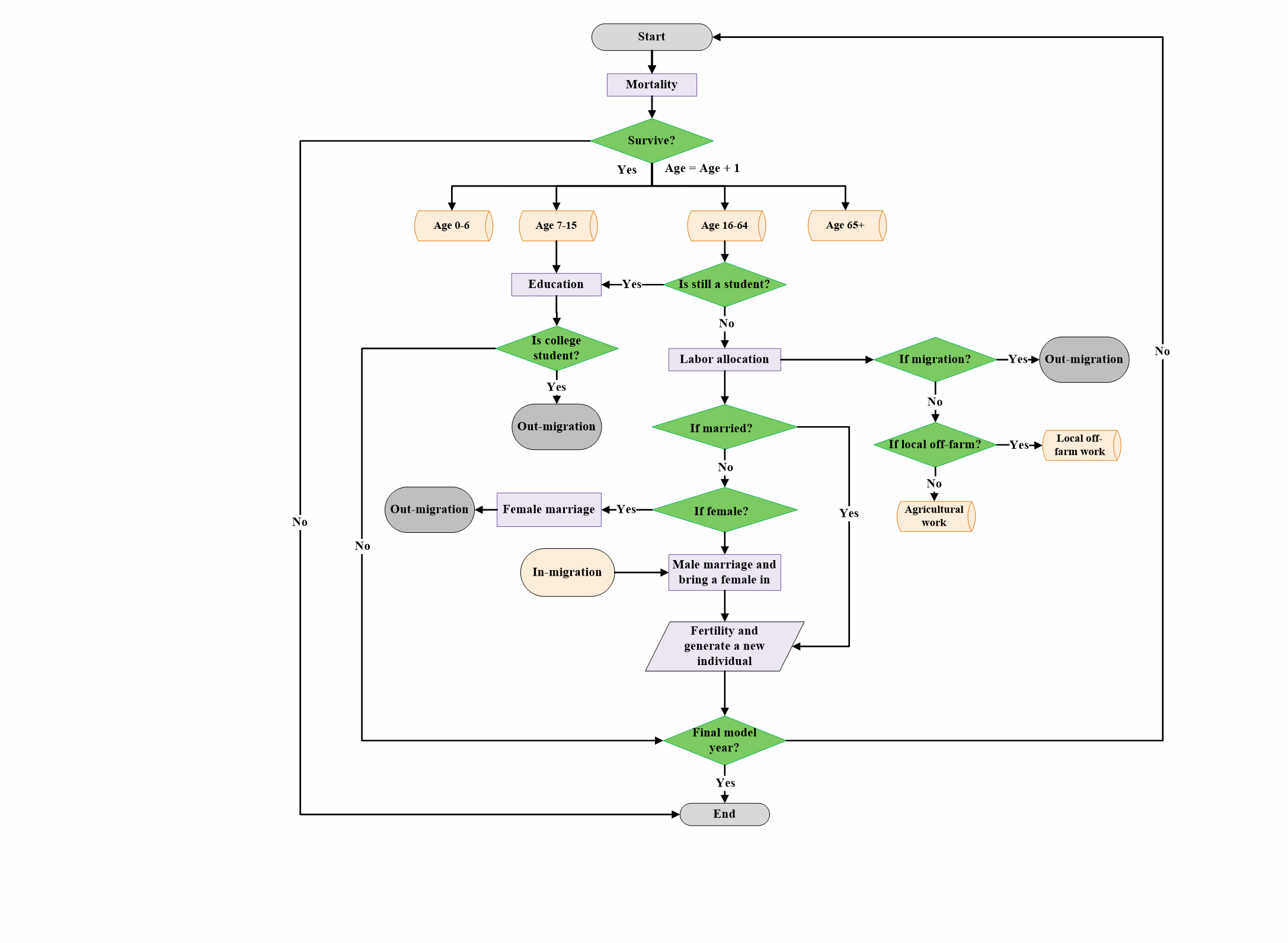
Then, an education submodule is executed for all students in the compulsory education stage (7-15 years old) and students aged between 16-21, who may attend high school or college. In rural China, children nowadays should receive 9 years of compulsory education, including primary school and middle school that are situated in local areas. Thus, for children in this stage, we just increase year of education by one during each time step. When they finish compulsory education, they need to decide whether to attend high-school and then college. We first predict the high-school and college enrollment rate based on historical education data derived from the Ministry of Education of the People’s Republic of China (Table 2). The equations predicting probability of high-school and college enrollments are shown below:
| \[P_{highschoolenrollment} = 25.73*e^{0.057}*(t+23); (R^{2} = 0.96)\] | \[(1)\] |
| \[P_{collegeenrollment} = 1.23+1.35*(t+23); (R^{2} = 0.98)\] | \[(2)\] |
where \(t\) is the time-step, \(t=0\) represents the model start year of 2014. The predicted enrollment rates are also listed in Table 5.
Then for each individual facing the choice of whether to continue education, we draw a random number between the interval of \([0,1]\) and compare it with the predicted high school or college enrollment rate. If the number is smaller than the rate, then the student continues attending school, otherwise, the person would join the labor force.
| Year | High School | College | ||
|---|---|---|---|---|
| Real data | Predicted | Real data | Predicted | |
| 1992 | 26.0 | 27.2 | 3.9 | 2.6 |
| 1993 | 28.4 | 28.8 | 5.0 | 3.9 |
| 1994 | 30.7 | 30.5 | 6.0 | 5.3 |
| 1995 | 33.6 | 32.3 | 7.2 | 6.6 |
| 1996 | 38.0 | 34.2 | 8.3 | 8.0 |
| 1997 | 40.6 | 36.2 | 9.1 | 9.3 |
| 1998 | 40.7 | 38.4 | 9.8 | 10.7 |
| 1999 | 41.0 | 40.6 | 10.5 | 12.0 |
| 2000 | 42.8 | 43.0 | 12.5 | 13.4 |
| 2001 | 42.8 | 45.5 | 13.3 | 14.7 |
| 2002 | 42.8 | 48.2 | 15.0 | 16.1 |
| 2003 | 43.8 | 51.0 | 17.0 | 17.4 |
| 2004 | 48.1 | 54.0 | 19.0 | 18.7 |
| 2005 | 52.7 | 57.2 | 21.0 | 20.1 |
| 2006 | 59.8 | 60.6 | 22.0 | 21.4 |
| 2007 | 66.0 | 64.1 | 23.0 | 22.8 |
| 2008 | 74.0 | 67.9 | 23.3 | 24.1 |
| 2009 | 79.2 | 71.9 | 24.2 | 25.5 |
| 2010 | 82.5 | 76.1 | 26.5 | 26.8 |
| 2011 | 84.0 | 80.6 | 26.9 | 28.2 |
| 2012 | 85.0 | 85.3 | 30.0 | 29.5 |
| 2013 | 86.0 | 90.4 | 34.5 | 30.9 |
A marriage submodule is applied to single adults who have reached the legal age of marriage (males \(\geq\) 22 and females \(\geq\) 20). The probability of marriage for male and female belonging to different age groups is obtained from household survey data (Table 6). Similarly, a random number is generated; if it is smaller than the marriage probability, then the individual get married.
| Gender | Range (year) | Probability (%) |
|---|---|---|
| Female | \(<20\) | Not legally allow to marry |
| \([20, 25)\) | 43.3 | |
| \([25,30)\) | 80.0 | |
| \([30, 100]\) | 100.0 | |
| Male | \(<22\) | Not legally allow to marry |
| \([22, 30)\) | 17.4 | |
| \([30, 35)\) | 37.0 | |
| \([35, 40)\) | 55.9 | |
| \([40, 45)\) | 85.3 | |
| \([45, 100]\) | 90.0 | |
A fertility submodule is applied to married females under 50 years old. In rural areas of China, factors influencing a couple’s fertility plan include the age of the female, number of children in the household, and if the household already has a male child. Based on empirical data, we apply a binary logistic regression to estimate the fertility intention of each couple based on the age of the female, number of children they already had and if they have a male child (Table 7), as shown below:
| \[log(\frac{P_{Yi}}{1-P_{Yi}}) = \alpha + \sum \beta_{k} x_{ik} + \epsilon_{i}\] | \[(3)\] |
where \(P_{Yi}\) denotes the predicted fertility intention for a married couple \(i\); \(x_{k}\) represents one of the explanatory factors affecting the fertility intention; \(\beta_{k}\) is the estimated coefficient for the kth factor, measuring the effect of the factor; and \(\epsilon\) is the error term. However, whether a couple would eventually give birth to a child is also affected by the birth rate and other random factors, which are also considered in the ABM-LLA model.
| Variable | \(\beta\) | S.E. | Wald | Sig. | \(e^{\beta}\) |
|---|---|---|---|---|---|
| Age | -0.148 | 0.038 | 15.447 | 0.000 | 0.863 |
| Number of children | -1.923 | 0.583 | 10.872 | 0.001 | 0.146 |
| If has a male child | -2.617 | 0.623 | 17.678 | 0.000 | 0.073 |
| Constant | 6.459 | 1.263 | 26.167 | 0.000 | 638.263 |
During the simulation of demographic processes, a migration submodule is applied to simulate out-migration and in-migration. Out-migration occurs when an individual moves out to receive high education, gets married or seeks jobs in cities. In-migration occurs when a male gets married and brings a female in, or migrants return. Migrants are still economically tied to their original households (e.g., remittances). Individual demographic processes may lead to changes in household demographic variables. Thus, an update procedure is called to update household’s member list, out-migrants list, household size, head’s age and education, household composition (number of members in different life stages), labor list, and number of labor-contributing adults (aged \(\geq\) 16).
Individual labor allocation module
If a household has labor-contributing adults, the model moves to the individual labor allocation module to simulate labor allocation behaviors. Although labor allocation decision is made at the individual level, the model considers a host of household- and RG-level factors in addition to individual attributes. If a household has no available labor, the household relies on remittances from out-migrants and/or government subsidies to survive. To simplify the model, we assume that each individual engages in only one of the three types of work during each time-step, i.e., on-farm work, local off-farm work, or migratory work. Here, we use two different rules to parameterize individual labor allocation.
The EK rule relies on empirical knowledge gained from the household survey data and implemented with empirical models. Although labor allocation decision is made at the individual level, the model considers a host of household- and RG-level factors in addition to individual attributes. We use the binary logistic regression to predict the probability for an individual to adopt local off-farm or migratory work based on factors including personal attributes, five dimensions of livelihood capitals and the policy context (i.e., CCFP and EWFP participations, ASP subsidies); \(\beta_{k}\) is the estimated coefficient for the kth factor, measuring the effect of the factor; and \(\epsilon\) is the error term. The estimated coefficients are listed in Table 3. Then the probabilistic approach is adopted to determine whether an individual adopt local off-farm or out-migration. The approach draws a random number in \([0,1]\) and compares it with the estimated probability, if the number is smaller than the portability, then the specific decision would be taken. If both decisions are not adopted, the person would prefer on-farm work.
Under the BR rule, individuals are assumed to use their limited information, experiences, and resources to make a perceived optimal choice. An individual estimates economic returns from the three types of work (on-farm, local off-farm, and out-migration) based on its own experience and that of its neighbors. Specifically, if an individual is a new labor who has just joined the labor force, he/she would make the labor allocation choice based primarily on information gathered from neighbors. The individual searches three other labor individuals at neighboring households, acquires information of their incomes for all possible livelihood activities including on-farm work, local off-farm work, remittances from out-migrants, and compare their incomes to select the job with the highest income. To account for a person’s ability as well as the randomness, the probabilistic approach is further adopted to decide whether an individual can eventually engage in the preferred work. Meanwhile, for an individual already involved in a type of work, his/her decision is about whether to change the job that would bring higher income. The individual searches three other neighboring individuals engaged in the other two types of work and would change his/her work if the highest neighboring individuals’ income is higher than the current income of the given person. It is worth mentioning that the number of neighbors that households seeking information on jobs is determined based on our household survey, i.e., “three” is the most frequent answer.
Under both rules, wages of households from local off-farm works and remittances sent by out-migrants are predicted based on statistical distributions derived from household survey data.
Household land allocation module
If a household has cropland parcels, then the land allocation module is executed to decide whether a household expands, maintains status quo or shrinks cultivated cropland area during each time-step. If the decision of cropland shrinkage is adopted, we further explore whether the shrinkage is through abandonment or renting-out (Wang et al. 2019). Logistic regression models are used to predict the probability for each decision. The selection of explanatory variables and estimation of parameters are introduced in detail in Wang et al. (2019). The M-logit model is used to predict the probability for a household to adopt stabilization, expansion, or shrinkage. Then, a B-logit model is applied to predict whether renting out or abandonment is further chosen. The estimated coefficients are also shown in Tables 8 and 9. The state variables of cropland parcel agents are updated after a household’s land allocation is made.
| Variables | Model-1 (refer to Stabilization) | ||||||
| Expand | Shrink | ||||||
| Coefficient | S.E. | P-value | Coefficient | S.E. | P-value | ||
| Policy context | CCFP | 0.545 | 0.793 | 0.236 | -0.005 | 0.346 | 0.988 |
| EWFP | -0.408 | 0.163 | 0.095* | -0.390 | 0.126 | 0.037** | |
| ASP | -0.301 | 0.204 | 0.276 | -0.243 | 0.163 | 0.242 | |
| Human | Household size | -0.473 | 0.159 | 0.064* | -0.546 | 0.133 | 0.018** |
| adults age | -0.282 | 0.232 | 0.359 | 0.207 | 0.299 | 0.395 | |
| Education of head | 0.085 | 0.314 | 0.768 | -0.422 | 0.138 | 0.045** | |
| Medical expense | -0.221 | 0.173 | 0.305 | -0.311 | 0.145 | 0.115 | |
| Non-farm labor | -1.194 | 0.137 | 0.008*** | -0.117 | 0.206 | 0.615 | |
| Migrants | 0.176 | 0.649 | 0.745 | 0.995 | 1.110 | 0.015** | |
| Natural | Cropland endowment | -0.540 | 0.207 | 0.129 | 0.852 | 0.567 | 0.000*** |
| Plot number | 0.230 | 0.327 | 0.376 | -0.711 | 0.120 | 0.004*** | |
| Walk time (plots) | -0.217 | 0.277 | 0.528 | 0.190 | 0.245 | 0.349 | |
| Physical | Farm tools | 0.729 | 0.726 | 0.037** | 0.109 | 0.247 | 0.622 |
| Transportation equipment | 0.734 | 0.585 | 0.009*** | 0.503 | 0.378 | 0.028*** | |
| Financial | Animal | 0.062 | 0.343 | 0.846 | -0.250 | 0.161 | 0.228 |
| If GE | -0.970 | 0.258 | 0.15 | -1.005 | 0.192 | 0.055* | |
| Remittance received | -0.124 | 0.235 | 0.639 | 0.054 | 0.230 | 0.804 | |
| Social | Social connect | 0.215 | 0.309 | 0.389 | 0.380 | 0.299 | 0.063* |
| Group size | -0.607 | 0.181 | 0.067* | -0.423 | 0.129 | 0.032** | |
| Group wellness | -0.387 | 0.212 | 0.214 | 0.118 | 0.211 | 0.531 | |
| Constant | -0.734 | 0.284 | 0.214 | 1.050 | 1.409 | 0.033*** | |
| Variables | Model-2 (refer to Renting out) | |||
|---|---|---|---|---|
| Abandon | ||||
| Coefficient | S.E. | P-value | ||
| Policy context | CCFP | -0.060 | 0.443 | 0.899 |
| EWFP | -0.084 | 0.197 | 0.695 | |
| ASP | -0.243 | 0.157 | 0.224 | |
| Human | Household size | 0.391 | 0.520 | 0.267 |
| adults age | -0.120 | 0.221 | 0.630 | |
| Education of head | -0.574 | 0.132 | 0.014** | |
| Medical expense | -0.496 | 0.158 | 0.056* | |
| Non-farm labor | -0.425 | 0.209 | 0.185 | |
| Migrants | -1.155 | 0.177 | 0.039** | |
| Natural | Cropland endowment | -0.454 | 0.165 | 0.080* |
| Plot number | 2.556 | 5.284 | 0.000*** | |
| Walk time (plots) | -0.305 | 0.182 | 0.216 | |
| Physical | Farm tools | -0.158 | 0.228 | 0.556 |
| Transportation equipment | 0.324 | 0.390 | 0.251 | |
| Financial | Animal | -0.411 | 0.155 | 0.078* |
| If GE | 0.523 | 0.855 | 0.302 | |
| Remittance received | 0.686 | 0.584 | 0.020** | |
| Social | Social connect | 0.146 | 0.307 | 0.582 |
| Group size | 0.359 | 0.354 | 0.147 | |
| Group wellness | -0.516 | 0.157 | 0.050* | |
| Constant | 1.816 | 4.071 | 0.006*** | |
| Model | Wald-Chi2 | p(Wald) | Pseudo-\(R^{2}\) |
|---|---|---|---|
| 1 | 99.30 | < 0.001 | 0.289 |
| 2 | 88.54 | < 0.001 | 0.474 |
Household assets module
After livelihood strategies and land use decisions are made, the household assets module is further adopted to calculate all sources of household incomes and expenses. Income sources include incomes from cereal and cash crop production, livestock, Gastrodia Elata cultivation, non-farm work, remittances from migrants, social gifts, and governmental subsidies. Expenses include agricultural inputs, food expense, utility expense (e.g., electricity), living goods expense (e.g., clothing), social gifts expense, education expense and medical expense. Accordingly, total income, expense and balance can be estimated. Based on the balance, a household decides whether to improve its overall wellness status, such as housing condition, farm tools, and transportation and communication equipment.
Specifically, the Cobb-Douglas production function is applied to estimate yields of crops based on age and education of household’s head, the number of agricultural labors, cropland area, expenses of fertilizers, pesticide, seeds, and hired labor
| \[Y_{crop} = e^{3.512+0.003Age-0.007Edu} x_{agrilabor}^{-0.263} x_{land}^{1.104} x_{fertil}^{0.1} x_{pest}^{-0.001} x_{seed}^{0.257} x_{hiredlabor}^{0.015}\] | \[(4)\] |
where \(x_{agrilabor}\), \(x_{land}\), \(x_{fertil}\), \(x_{pest}\), \(x_{seed}\), \(x_{hiredlabor}\) are the number of agricultural labor, cropland area, expenses of fertilizers, pesticide, seeds, and hired labor, respectively. Here, we assume crop yield increases by 5% per year due to technology improvement. Then the net income can be estimated based on crop yield and price, and agricultural input expenses.
Similarly, the income of Gastrodia Elata (\(Y_{GE}\)) can be calculated based on Cobb-Douglas production functions using the household data with the following equation:
| \[Y_{GE}=e^{8.164-0.024Age+0.026Edu} x_{agrilabor}^{0.390} x_{GEseed}^{0.151}\] | \[(5)\] |
where \(x_{GEseed}\) is the seed expense of Gastrodia Elata cultivation.
Major expenses include agricultural inputs, food expense, utility expense (e.g., electricity), living goods expense (e.g., clothing), and education expense. Accordingly, total income, expense and balance can be estimated. Based on the balance, a household decides whether to improve its overall wellness status, such as housing condition, farm tools, and transportation and communication equipment.
Appendix 2: Questionnaire for Evaluating Level of Household Wellness
The index was computed by summing highest points corresponding to house entry in each category.
| Category | Item | Points | |
|---|---|---|---|
| 1 | What type of house do you have? | Three story concrete | 5 |
| Two story concrete with indoor bathroom | 4 | ||
| Two story concrete without indoor bathroom | 3 | ||
| Single story Brick House | 2 | ||
| Adobe house | 1 | ||
| No house | 0 | ||
| 2 | What kind of fuel do you use? | Coal, gas or electricity only, no fuelwood | 5 |
| Primarily coal, gas & electricity, some fuelwood | 4 | ||
| About half coal, gas & electricity, half fuelwood | 3 | ||
| Primarily fuelwood, some coal, gas & electricity | 2 | ||
| Fuelwood only | 1 | ||
| Rice, wheat, or corn stalks only | 0 | ||
| 3 | What kind of water and sanitation facilities do you have? | Piped water and flush toilet | 5 |
| Piped water and outdoor latrine | 4 | ||
| Pressure well and outdoor latrine | 3 | ||
| Natural Spring and outdoor latrine | 2 | ||
| Open water and outdoor latrine | 1 | ||
| Harvest rain and outdoor latrine | 0 | ||
| 4 | What kind of electrical appliances do you have? | A/C in house | 5 |
| Solar panel | 4 | ||
| Refrigerator | 3 | ||
| Washing/Dry machine | 2 | ||
| Electric cooking pot/microwave | 1 | ||
| None | 0 | ||
| 5 | What communications and entertainment equipment do you have? | Computer | 5 |
| Cell phone | 4 | ||
| Fixed line phone | 3 | ||
| TV/Stereo | 2 | ||
| Radio | 1 | ||
| None | 0 | ||
| 6 | What farm tools and equipment do you have? | Tractor/transporting tractor (>2000 Yuan) | 5 |
| Thrasher machine/Other small process machine | 4 | ||
| Electric pump | 3 | ||
| Ox | 2 | ||
| Hoes, other farm tools | 1 | ||
| None | 0 | ||
| 7 | What do you use for transportation? | Sedan or minivan | 5 |
| Mini-truck | 4 | ||
| Motor cycle/Motorized tricycle | 3 | ||
| Electric bike | 2 | ||
| Bike or human-powered tricycle | 1 | ||
| None | 0 | ||
Appendix 3: Other Model Outputs
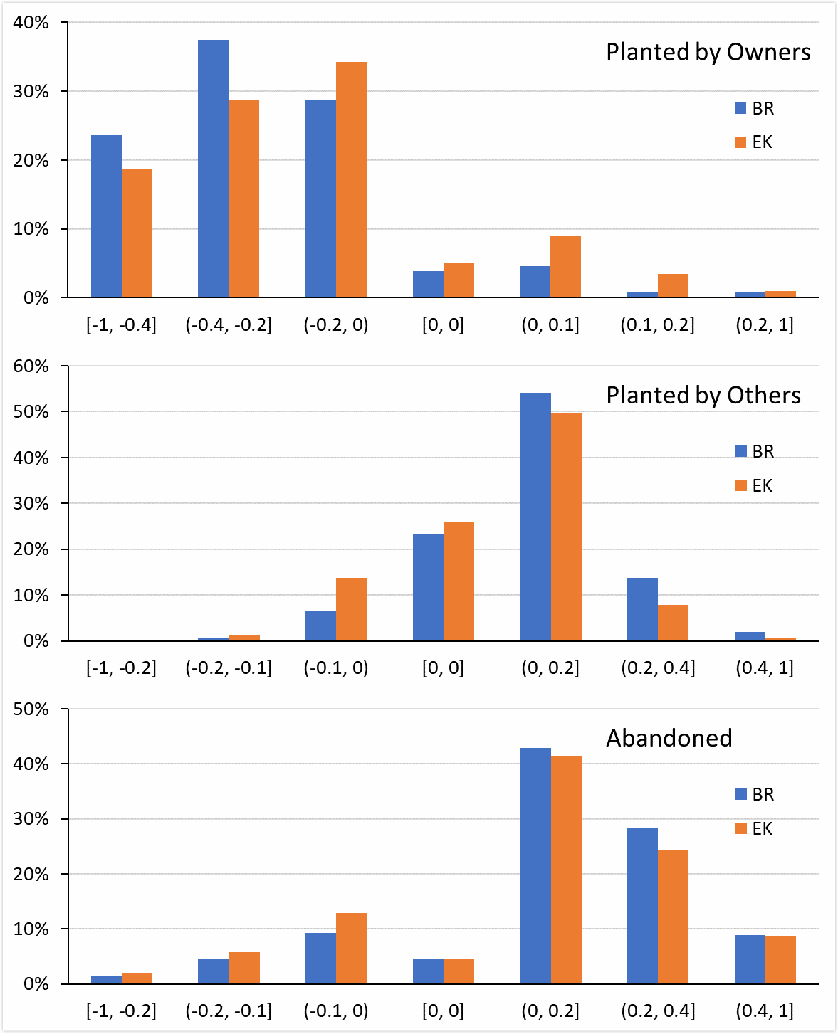
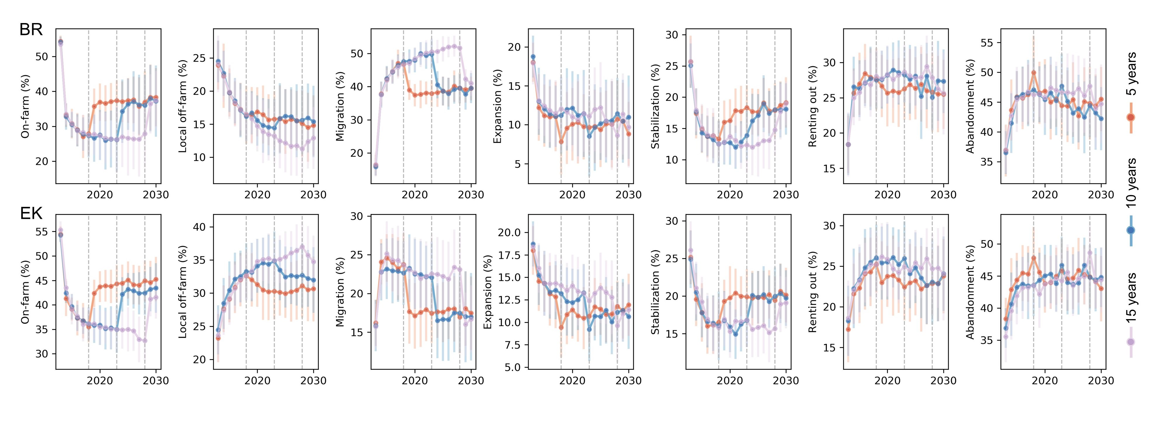
References
AMADOU, M. L., Villamor, G. B., & Kyei-Baffour, N. (2018). Simulating agricultural land-use adaptation decisions to climate change: An empirical agent-based modelling in northern Ghana. Agricultural Systems, 166, 196–209. [doi:10.1016/j.agsy.2017.10.015]
AN, L. (2012). Modeling human decisions in coupled human and natural systems: Review of agent-based models. Ecological Modelling, 229, 25–36. [doi:10.1016/j.ecolmodel.2011.07.010]
AN, L., Linderman, M., Qi, J., Shortridge, A., & Liu, J. (2005). Exploring complexity in a human–environment system: An agent-based spatial model for multidisciplinary and multiscale integration. Annals of the Association of American Geographers, 95(1), 54–79. [doi:10.1111/j.1467-8306.2005.00450.x]
AN, L., Mak, J., Yang, S., Lewison, R., Stow, D. A., Chen, H. L., Xu, W., & Tsai, Y. H. (2020). Cascading impacts of payments for ecosystem services in complex human-Environment systems. Journal of Artificial Societies and Social Simulation, 23(1), 5: https://www.jasss.org/23/1/5.html. [doi:10.18564/jasss.4196]
AN, L., Zvoleff, A., Liu, J., & Axinn, W. (2014). Agent-Based modeling in coupled human and natural systems (CHANS): Lessons from a comparative analysis. Annals of the Association of American Geographers, 104(4), 723–745. [doi:10.1080/00045608.2014.910085]
APPEL, F., & Balmann, A. (2019). Human behaviour versus optimising agents and the resilience of farms – Insights from agent-based participatory experiments with FarmAgriPoliS. Ecological Complexity, 40, 100731. [doi:10.1016/j.ecocom.2018.08.005]
BERGER, T., Troost, C., Wossen, T., Latynskiy, E., Tesfaye, K., & Gbegbelegbe, S. (2017). Can smallholder farmers adapt to climate variability, and how effective are policy interventions? Agent-based simulation results for Ethiopia. Agricultural Economics, 48(6), 693–706. [doi:10.1111/agec.12367]
BERNOULLI, D. (1954). Exposition of a new theory on the measurement of risk. Econometrica, 22(1), 23–36.
BOERO, R., & Squazzoni, F. (2005). Does empirical embeddedness matter? Methodological issues on agent-based models for analytical social science. Journal of Artificial Societies and Social Simulation, 8(4), 6: https://www.jasss.org/8/4/6.html.
BRYAN, B. A., Gao, L., Ye, Y., Sun, X., Connor, J. D., Crossman, N. D., Stafford-Smith, M., Wu, J., He, C., Yu, D., Liu, Z., Huang, Q., Ren, H., Deng, X., Zheng, H., Niu, J., Han, G., & Hou, X. (2018). China’s response to a national land-system sustainability emergency. Nature, 559(7713), 193–204. [doi:10.1038/s41586-018-0280-2]
CARTER, N. H., Viña, A., Hull, V., McConnell, W. J., Axinn, W., Ghimire, D., & Liu, J. (2014). Coupled human and natural systems approach to wildlife research and conservation. Ecology and Society, 19(3), 43. [doi:10.5751/es-06881-190343]
CHEN, X., Lupi, F., He, G., & Liu, J. (2009). Linking social norms to efficient conservation investment in payments for ecosystem services. Proceedings of the National Academy of Sciences, 106(28), 11812–11817. [doi:10.1073/pnas.0809980106]
CHINA State Council. (2002). The guidelines for conversion of cropland to forest. State council executive order No. 367. Retrieved from: http://www.forestry.gov.cn/main/3706/20021214/566706.html
CHINA State Council. (2003). Directive to enhance forestry development. Issue 25. Retrieved from: http://www.gov.cn/gongbao/content/2003/content_62358.html
DAI, L., Zhao, F., Shao, G., Zhou, L., & Tang, L. (2009). China’s classification-based forest management: Procedures, problems, and prospects. Environmental Management, 43(6), 1162–1173. [doi:10.1007/s00267-008-9229-9]
DELGADO-AGUILAR, M. J., Hinojosa, L., & Schmitt, C. B. (2019). Combining remote sensing techniques and participatory mapping to understand the relations between forest degradation and ecosystems services in a tropical rainforest. Applied Geography, 104, 65–74. [doi:10.1016/j.apgeog.2019.02.003]
DENG, J., Sun, P., Zhao, F., Han, X., Yang, G., & Feng, Y. (2016). Analysis of the ecological conservation behavior of farmers in payment for ecosystem service programs in eco-environmentally fragile areas using social psychology models. Science of the Total Environment, 550, 382–390. [doi:10.1016/j.scitotenv.2016.01.152]
DÉMURGER, S., & Wan, H. (2012). Payments for ecological restoration and internal migration in China: The sloping land conversion program in Ningxia. IZA Journal of Migration, 1(1), 10.
DFID. (1999). DFID-sustainable livelihoods guidance sheets. Available at: https://www.ennonline.net/dfidsustainableliving.
DOU, Y., Deadman, P. J., Berbés-Blázquez, M., Vogt, N. D., & Almeida, O. (2020). Pathways out of poverty through the lens of development resilience: An agent-based simulation. Ecology and Society, 25(4), 3. [doi:10.5751/es-11842-250403]
DOU, Y., Yao, G., Herzberger, A., da Silva, R. F. B., Song, Q., Hovis, C., Batistella, M., Moran, E., Wu, W., & Liu, J. (2020). Land-Use changes in distant places: Implementation of a telecoupled agent-Based model. Journal of Artificial Societies and Social Simulation, 23(1), 11: https://www.jasss.org/23/3/11.html. [doi:10.18564/jasss.4211]
DRESSLER, G., Groeneveld, J., Buchmann, C. M., Guo, C., Hase, N., Thober, J., Frank, K., & Müller, B. (2019). Implications of behavioral change for the resilience of pastoral systems - Lessons from an agent-based model. Ecological Complexity, 40, 1–13. [doi:10.1016/j.ecocom.2018.06.002]
ELSAWAH, S., Guillaume, J. H., Filatova, T., Rook, J., & Jakeman, A. J. (2015). A methodology for eliciting, representing, and analysing stakeholder knowledge for decision making on complex socio-ecological systems: From cognitive maps to agent-based models. Journal of Environmental Management, 151, 500–516. [doi:10.1016/j.jenvman.2014.11.028]
ENTWISLE, B., Walsh, S. J., Rindfuss, R. R., & Chamratrithirong, A. (1998). 'Land-use/land-cover and population dynamics, Nang Rong, Thailand.' In B. Entwisle & P. C. Stern (Eds.), Population, Land Use, and Environment: Research Directions. Washington, DC: National Academy Press. [doi:10.3886/icpsr04402]
ENTWISLE, B., Williams, N. E., Verdery, A. M., Rindfuss, R. R., Walsh, S. J., Malanson, G. P., Mucha, P. J., Frizzelle, B. G., McDaniel, P. M., Yao, X., Heumann, B. H., Prasartkul, P., Sawangdee, Y., & Jampaklay, A. (2016). Climate shocks and migration: An agent-Based modeling approach. Population and Environment, 38(1), 47–71. [doi:10.1007/s11111-016-0254-y]
FILATOVA, T., Polhill, J. G., & van Ewijk, S. (2016). Regime shifts in coupled socio-environmental systems: Review of modelling challenges and approaches. Environmental Modelling & Software, 75, 333–347. [doi:10.1016/j.envsoft.2015.04.003]
FILATOVA, T., Verburg, P. H., Parker, D. C., & Stannard, C. A. (2013). Spatial agent-based models for socio-ecological systems: Challenges and prospects. Environmental Modelling & Software, 45, 1–7. [doi:10.1016/j.envsoft.2013.03.017]
FOLEY, J. A., Defries, R., Asner, G. P., Barford, C., Bonan, G., Carpenter, S. R., Chapin, F. S., Coe, M. T., Daily, G. C., Gibbs, H. K., Helkowski, J. H., Holloway, T., Howard, E. A., Kucharik, C. J., Monfreda, C., Patz, J. A., Prentice, I. C., Ramankutty, N., & Snyder, P. K. (2005). Global consequences of land use. Science, 309(5734), 570–574. [doi:10.1126/science.1111772]
GOTTS, N. M., & Polhill, J. G. (2009). When and how to imitate your neighbours: Lessons from and for FEARLUS. Journal of Artificial Societies and Social Simulation, 12(3), 2: https://www.jasss.org/12/3/2.html.
GRANCO, G., Heier Stamm, J. L., Bergtold, J. S., Daniels, M. D., Sanderson, M. R., Sheshukov, A. Y., Mather, M. E., Caldas, M. M., Ramsey, S. M., Lehrter II, R. J., Haukos, D. A., Gao, J., Chatterjee, S., Nifong, J. C., & Aistrup, J. A. (2019). Evaluating environmental change and behavioral decision-making for sustainability policy using an agent-based model: A case study for the Smoky Hill River Watershed, Kansas. Science of the Total Environment, 695, 133769. [doi:10.1016/j.scitotenv.2019.133769]
GRIMM, V., Berger, U., Bastiansen, F., Eliassen, S., Ginot, V., Giske, J., Goss-Custard, J., Grand, T., Heinz, S. K., Huse, G., Huth, A., Jepsen, J. U., Jørgensen, C., Mooij, W. M., Müller, B., Pe’er, G., Piou, C., Railsback, S. F., Robbins, A. W., … DeAngelis, D. L. (2006). A standard protocol for describing individual-based and agent-based models. Ecological Modelling, 198(1–2), 115–126. [doi:10.1016/j.ecolmodel.2006.04.023]
GRIMM, V., Berger, U., DeAngelis, D. L., Polhill, J. G., Giske, J., & Railsback, S. F. (2010). The ODD protocol: A review and first update. Ecological Modelling, 221(23), 2760–2768. [doi:10.1016/j.ecolmodel.2010.08.019]
GROENEVELD, J., Müller, B., Buchmann, C. M., Dressler, G., Guo, C., Hase, N., Hoffmann, F., John, F., Klassert, C., Lauf, T., Liebelt, V., Nolzen, H., Pannicke, N., Schulze, J., Weise, H., & Schwarz, N. (2017). Theoretical foundations of human decision-making in agent-based land use models – A review. Environmental Modelling & Software, 87, 39–48. [doi:10.1016/j.envsoft.2016.10.008]
GUO, Y., Zhou, Y., & Liu, Y. (2019). Targeted poverty alleviation and its practices in rural China: A case study of Fuping county, Hebei Province. Journal of Rural Studies, 1–10. [doi:10.1016/j.jrurstud.2019.01.007]
HAER, T., Husby, T. G., Botzen, W. J. W., & Aerts, J. C. J. H. (2020). The safe development paradox: An agent-based model for flood risk under climate change in the European Union. Global Environmental Change, 60, 1–12. [doi:10.1016/j.gloenvcha.2019.102009]
HAUCK, J., Schmidt, J., & Werner, A. (2016). Using social network analysis to identify key stakeholders in agricultural biodiversity governance and related land-use decisions at regional and local level. Ecology and Society, 21(2), 49. [doi:10.5751/es-08596-210249]
HEPPENSTALL, A., Crooks, A., Malleson, N., Manley, E., Ge, J., & Batty, M. (2021). Future developments in geographical agent-Based models: Challenges and opportunities. Geographical Anaalysis, 53(1), 76–91. [doi:10.1111/gean.12267]
HUANG, J., Wang, X., Zhi, H., HUANG, Z., & Rozelle, S. (2011). Subsidies and distortions in China’s agriculture: Evidence from producer-level data. Australian Journal of Agricultural and Resource Economics, 55(1), 53–71. [doi:10.1111/j.1467-8489.2010.00527.x]
HUANG, J., & Yang, G. (2017). Understanding recent challenges and new food policy in China. Global Food Security, 12, 119–126. [doi:10.1016/j.gfs.2016.10.002]
JANSSEN, M., & Ostrom, E. (2006). Empirically based, agent-based models. Ecology and Society, 11(2), 37. [doi:10.5751/es-01861-110237]
JIANG, S., Alves, A., Rodrigues, F., Ferreira, J., & Pereira, F. C. (2015). Mining point-of-interest data from social networks for urban land use classification and disaggregation. Computers, Environment and Urban Systems, 53, 36–46. [doi:10.1016/j.compenvurbsys.2014.12.001]
KHAN, S., Hanjra, M. A., & Mu, J. (2009). Water management and crop production for food security in China: A review. Agricultural Water Management, 96(349–360), 3. [doi:10.1016/j.agwat.2008.09.022]
KONG, W. (2016). The Study on the Managing Policies of China’s Agriculture Market. Diploma thesis: Chinese Academy of Agricultural Sciences (in Chinese).
KREMMYDAS, D., Athanasiadis, I. N., & Rozakis, S. (2018). A review of agent based modeling for agricultural policy evaluation. Agricultural Systems, 164, 95–106. [doi:10.1016/j.agsy.2018.03.010]
LE, Q. B., Park, S. J., & Vlek, P. L. G. (2010). Land use dynamic simulator (LUDAS): A multi-agent system model for simulating spatio-temporal dynamics of coupled human–landscape system. Ecological Informatics, 5(3), 203–221. [doi:10.1016/j.ecoinf.2010.02.001]
LI, Q., Amjath Babu, T. S., Sieber, S., & Zander, P. (2018). Assessing divergent consequences of payments for ecosystem services on rural livelihoods: A case-study in China’s Loess Hills. Land Degradation & Development, 29(10), 3549–3570. [doi:10.1002/ldr.3082]
LI, Q., & Zander, P. (2019). Resilience building of rural livelihoods in PES programmes: A case study in China’s Loess Hills. Ambio, 49, 962–985. [doi:10.1007/s13280-019-01236-4]
LI, S., Liu, X., Paudel, B., Xu, F., & Deng, Q. (2020). Stable sediment retention and rapid economic growth occurred together from the end of the 1970s to 2015 in the Three Gorges Reservoir area. Land Degradation & Development. [doi:10.1002/ldr.3818]
LIU, C., Lü, J., & Yin, R. (2009). An estimation of the effects of China’s forestry programs on farmers’ income. In R. Yin (Ed.), An integrated assessment of China’s ecological restoration programs (pp. 201–218). Springer. [doi:10.1007/978-90-481-2655-2_12]
LIU, G., Wang, H., Cheng, Y., Zheng, B., & Lu, Z. (2016). The impact of rural out-migration on arable land use intensity: Evidence from mountain areas in Guangdong, China. Land Use Policy, 59, 569–579. [doi:10.1016/j.landusepol.2016.10.005]
LIU, J., & Diamond, J. (2005). China’s environment in a globalizing world. Nature, 435(7046), 1179–1186. [doi:10.1038/4351179a]
LIU, J., Dietz, T., Carpenter, S. R., Alberti, M., Folke, C., Moran, E., Pell, A. N., Deadman, P., Kratz, T., Lubchenco, J., Ostrom, E., Ouyang, Z., Provencher, W., Redman, C. L., Schneider, S. H., & Taylor, W. W. (2007). Complexity of coupled human and natural systems. Science, 317(5844), 1513–1516. [doi:10.1126/science.1144004]
LIU, K., Huisingh, D., Zhu, J., Ma, Y., O’Connor, D., & Hou, D. (2018). Farmers’ perceptions and adaptation behaviours concerning land degradation: A theoretical framework and a case-study in the Qinghai-Tibetan Plateau of China. Land Degradation & Development, 29(8), 2460–2471. [doi:10.1002/ldr.3011]
LIU, Y., LIU, J., & Zhou, Y. (2005). Spatio-temporal patterns of rural poverty in China and targeted poverty alleviation strategies. Journal of Rural Studies, 52, 66–75. [doi:10.1016/j.jrurstud.2017.04.002]
LV, G., & Li, Y. (2017). The story behind the wage growth over productivity growth: an empirical research based on privincial pannel model. Journal of Beijing Normal University (Social Sciences), 3, 83-98 (in Chinese).
MESHESHA, D. T., Tsunekawa, A., & Tsubo, M. (2012). Continuing land degradation: Cause-effect in Ethiopia’s Central Rift Valley. Land Degradation & Development, 23(2), 130–143. [doi:10.1002/ldr.1061]
MIYASAKA, T., Le, Q. B., Okuro, T., Zhao, X., & Takeuchi, K. (2017). Agent-based modeling of complex social–ecological feedback loops to assess multi-dimensional trade-offs in dryland ecosystem services. Landscape Ecology, 32(4), 707–727. [doi:10.1007/s10980-017-0495-x]
MONTICINO, M., Acevedo, M., Callicott, B., Cogdill, T., & Lindquist, C. (2007). Coupled human and natural systems: A multi-agent-based approach. Environmental Modelling & Software, 22(5), 656–663. [doi:10.1016/j.envsoft.2005.12.017]
MORRIS, C. (2004). Networks of agri-environmental policy implementation: A case study of England’s countryside stewardship scheme. Land Use Policy, 21(2), 177–191. [doi:10.1016/j.landusepol.2003.01.002]
ORCHARD, S. E., Stringer, L. C., & Manyatsi, A. M. (2017). Farmer perceptions and responses to soil degradation in Swaziland. Land Degradation & Development, 28(1), 46–56. [doi:10.1002/ldr.2595]
PIAO, S., Ciais, P., Huang, Y., Shen, Z., Peng, S., Li, J., Zhou, L., Liu, H., Ma, Y., Ding, Y., Friedlingstein, P., Liu, C., Tan, K., Yu, Y., Zhang, T., & Fang, J. (2010). The impacts of climate change on water resources and agriculture in China. Nature, 467(7311), 43–51. [doi:10.1038/nature09364]
POLHILL, J. G., Gotts, N. M., & Law, A. N. R. (2001). Imitative versus nonimitative strategies in a land-use simulation. Cybernetics & Systems, 32(1–2), 285–307.
POOT, J., Waldorf, B., & van Wissen, L. (2009). Migration and Human Capital. Cheltenham: Edward Elgar Publishing.
RINDFUSS, R., Entwisle, B., Walsh, S., An, L., Badenoch, N., Brown, D., Deadman, P., Evans, T., Fox, J., Geoghegan, J., Gutmann, M., Kelly, M., Linderman, M., Liu, J., Malanson, G., Mena, C., Messina, J., Moran, E., Parker, D., & Verburg, P. (2008). Land use change: Complexity and comparisons. Journal of Land Use Science, 1(1), 1–10. [doi:10.1080/17474230802047955]
SANJUÁN, Y., Gómez-Villar, A., Nadal-Romero, E., Álvarez-Martínez, J., Arnáez, J., Serrano-Muela, M. P., Rubiales, J. M., González-Sampériz, P., & García-Ruiz, J. M. (2016). Linking land cover changes in the Sub-Alpine and Montane Belts to changes in a torrential river. Land Degradation & Development, 27(2), 179–189.
SCHOUTEN, M., Verwaart, T., & Heijman, W. (2014). Comparing two sensitivity analysis approaches for two scenarios with a spatially explicit rural agent-based model. Environmental Modelling & Software, 54, 196–210. [doi:10.1016/j.envsoft.2014.01.003]
SIMON, H. A. (1972). Theories of bounded rationality. Decision and Organization, 1(1), 161–176.
SMAJGL, A., & Barreteau, O. (2014). Empirical Agent-Based Modelling: Challenges and Solutions. New York, NY: Springer.
SONG, C., Zhang, Y., Mei, Y., Liu, H., Zhang, Z., Zhang, Q., Zha, T., Zhang, K., Huang, C., Xu, X., Jagger, P., Chen, X., & Bilsborrow, R. (2014). Sustainability of forests created by China’s sloping land conversion program: A comparison among three sites in Anhui, Hubei and Shanxi. Forest Policy and Economics, 38, 161–167. [doi:10.1016/j.forpol.2013.08.012]
STATE Forestry Administration. (201). Approaches for national ecological welfare forest identification. Forest Policy No.88. Retrieved from: http://m.law-lib.com/law/law_view.asp?id=73395.
STATE Forestry Administration. (2015). Notice of the implementation of second round national conversion of cropland to forest and grassland. Ministry of Finance and Agriculture No.258. Retrieved from: http://www.forestry.gov.cn/tghl/4608/20200221/113438580931645.html.
SU, Y., Araral, E., & Wang, Y. (2020). The effects of farmland use rights trading and labor outmigration on the governance of the irrigation commons: Evidence from China. Land Use Policy, 91, 1–11. [doi:10.1016/j.landusepol.2019.104378]
SUN, Z., Lorscheid, I., Millington, J. D., Lauf, S., Magliocca, N. R., Groeneveld, J., Balbi, S., Nolzen, H., Mäller, B., Schulze, J., & Buchmann, C. M. (2016). Simple or complicated agent-based models? A complicated issue. Environmental Modelling & Software, 86, 56–67. [doi:10.1016/j.envsoft.2016.09.006]
TIAN, Q., Holland, J. H., & Brown, D. G. (2016). Social and economic impacts of subsidy policies on rural development in the Poyang Lake Region, China: Insights from an agent-based model. Agricultural Systems, 148, 12–27. [doi:10.1016/j.agsy.2016.06.005]
UCHIDA, E., Rozelle, S., & Xu, J. (2009). Conservation payments, liquidity constraints, and off-farm labor: Impact of the Grain-for-Green Program on rural households in China. American Journal of Agricultural Economics, 91(1), 70–86. [doi:10.1111/j.1467-8276.2008.01184.x]
VAN Schmidt, N. D., Kovach, T., Kilpatrick, A. M., Oviedo, J. L., Huntsinger, L., Hruska, T., Miller, N. L., & Beissinger, S. R. (2019). Integrating social and ecological data to model metapopulation dynamics in coupled human and natural systems. Ecology, 100(6), e02711. [doi:10.1002/ecy.2711]
WALSH, S. J., Malanson, G. P., Entwisle, B., Rindfuss, R. R., Mucha, P. J., Heumann, B. W., McDaniel, P., Frizzelle, B. G., Verdery, A. M., Williams, N. E., Xiao-Zheng, Y., & Ding, D. (2013). Design of an agent-Based model to examine population-Environment interactions in Nang Rong District, Thailand. Applied Geography, 39(6), 183–198. [doi:10.1016/j.apgeog.2012.12.010]
WALSH, S. J., Messina, J. P., Mena, C. F., Malanson, G. P., & Page, P. H. (2008). Complexity theory, spatial simulation models, and land use dynamics in the Northern Ecuadorian Amazon. Geoforum, 39(2), 867–878. [doi:10.1016/j.geoforum.2007.02.011]
WANG, Q., & Zhang, X. (2017). Three rights separation: China’s proposed rural land rights reform and four types of local trials. Land Use Policy, 63, 111–121. [doi:10.1016/j.landusepol.2017.01.027]
WANG, Y., Bilsborrow, R. E., Zhang, Q., Li, J., & Song, C. (2019). Effects of payment for ecosystem services and agricultural subsidy programs on rural household land use decisions in China: Synergy or trade-off? Land Use Policy, 81, 785–801. [doi:10.1016/j.landusepol.2018.10.057]
WANG, Y., Chen, C., & Araral, E. (2016). The effects of migration on collective action in the commons: Evidence from rural China. World Development, 88, 79–93. [doi:10.1016/j.worlddev.2016.07.014]
WANG, Y., Zhang, Q., Bilsborrow, R., Tao, S., Chen, X., Sullivan-Wiley, K., Huang, Q., Li, J., & Song, C. (2020). Effects of payments for ecosystem services programs in China on rural household labor allocation and land use: Identifying complex pathways. Land Use Policy, 99, 105024. [doi:10.1016/j.landusepol.2020.105024]
WEST, T. A. P., Grogan, K. A., Swisher, M. E., Caviglia-Harris, J. L., Sills, E. O., Roberts, D. A., Harris, D., & Putz, F. E. (2018). Impacts of REDD+ payments on a coupled human-natural system in Amazonia. Ecosystem Services, 33, 68–76. [doi:10.1016/j.ecoser.2018.08.008]
WILENSKY, U. (1999). NetLogo. Evanston, IL: Center for connected learning and computer-based modeling, Northwestern University.
WINDRUM, P., Fagiolo, G., & Moneta, A. (2007). Empirical validation of agent-Based models: Alternatives and prospects. Journal of Artificial Societies and Social Simulation, 10(2), 8: https://www.jasss.org/10/2/28.html.
XU, Y., Huang, X., Bao, H. X. H., Ju, X., Zhong, T., Chen, Z., & Zhou, Y. (2018). Rural land rights reform and agro-environmental sustainability: Empirical evidence from China. Land Use Policy, 74, 73–87. [doi:10.1016/j.landusepol.2017.07.038]
YAMASHITA, R., & Hoshino, S. (2018). Development of an agent-based model for estimation of agricultural land preservation in rural Japan. Agricultural Systems, 164, 264–276. [doi:10.1016/j.agsy.2018.05.004]
YANG, Z. (2013). Demographic changes in China’s farmers: The future of farming in China. Asian Social Science, 9(7), 136–143. [doi:10.5539/ass.v9n7p136]
YE, L., Xiong, W., Li, Z., Yang, P., Wu, W., Yang, G., Fu, Y., Zou, J., Chen, Z., van Ranst, E., & Tang, H. (2013). Climate change impact on China food security in 2050. Agronomy for Sustainable Development, 33(2), 363–374. [doi:10.1007/s13593-012-0102-0]
YI, F., Lu, W., & Zhou, Y. (2016). Cash transfers and multiplier effect: Lessons from the grain subsidy program in China. China Agricultural Economic Review, 8(1), 81–99. [doi:10.1108/caer-07-2015-0078]
ZHANG, P., Shao, G., Zhao, G., Le Master, D. C., Parker, G. R., Dunning Jr., J. B., & Li, Q. (2000). China’s forest policy for the 21st century. Science, 288(5474), 2135–2136. [doi:10.1126/science.288.5474.2135]
ZHANG, Q., Bilsborrow, R. E., Song, C., Tao, S., & Huang, Q. (2018). Determinants of out-migration in rural China: Effects of payments for ecosystem services. Population and Environment, 40(2), 182–203. [doi:10.1007/s11111-018-0307-5]
ZHANG, Q., Song, C., & Chen, X. (2018). Effects of China’s payment for ecosystem services programs on cropland abandonment: A case study in Tiantangzhai Township, Anhui, China. Land Use Policy, 73, 239–248. [doi:10.1016/j.landusepol.2018.01.001]
ZHOU, Y., & Liu, Y. (2019). The geography of poverty: Review and research prospects. Journal of Rural Studies.
ZVOLEFF, A., & An, L. (2014). The effect of reciprocal connections between demographic decision making and land use on decadal dynamics of population and land-use change. Ecology and Society, 19(31), 2. [doi:10.5751/es-06243-190231]