Multimodal Evolutionary Algorithms for Easing the Complexity of Agent-Based Model Calibration

, ,
and
aDepartment of Computer Science and Artificial Intelligence, Andalusian Research Institute in Data Science and Computational Intelligence, DaSCI, University of Granada, Spain; bSchool of Electrical Engineering and Computing, The University of Newcastle, Australia
Journal of Artificial
Societies and Social Simulation 24 (3) 4
<https://www.jasss.org/24/3/4.html>
DOI: 10.18564/jasss.4606
Received: 28-May-2020 Accepted: 21-Apr-2021 Published: 30-Jun-2021
Abstract
Agent-based modelling usually involves a calibration stage where a set of parameters needs to be estimated. The calibration process can be automatically performed by using calibration algorithms which search for an optimal parameter configuration to obtain quality model fittings. This issue makes the use of multimodal optimisation methods interesting for calibration as they can provide diverse solution sets with similar and optimal fitness. In this contribution, we compare nine competitive multimodal evolutionary algorithms, both classical and recent, to calibrate agent-based models. We analyse the performance of each multimodal evolutionary algorithm on 12 problem instances of an agent-based model for marketing (i.e. 12 different virtual markets) where we calibrate 24 to 129 parameters to generate two main outputs: historical brand awareness and word-of-mouth volume. Our study shows a clear dominance of SHADE, L-SHADE, and NichePSO over the rest of the multimodal evolutionary algorithms. We also highlight the benefits of these methods for helping modellers to choose from among the best calibrated solutions.Introduction
Agent-based modelling (Gilbert & Troitzsch 2005; Wilensky & Rand 2015) is a well-established paradigm for the design of computational models that rely on autonomous entities called agents. This paradigm allows the simulation of complex systems by aggregating the individual-level interactions through the underlying artificial social network of agents, creating high level outcomes and incorporating individual behavioural rules without higher level assumptions (Chica et al. 2018). When a model is correctly built, experts can then use it as a decision support system to evaluate their policies in what-if scenarios and understand how its target system works (Chica & Rand 2017). However, building agent-based models (ABMs) is a complex task since modellers normally have to set the values of a large number of parameters which are usually unknown.
The process of adjusting the parameter values of an ABM to correctly replicate the desired dynamics is known as calibration and is a crucial step during model validation (Oliva 2003). A commonly used approach is automatic calibration, which considers an error measure for comparing real-world data to the simulated model’s output and tunes a set of parameters of the model to match the data (Oliva 2003; Sargent 2005). Automated calibration normally requires an optimisation method for modifying the parameters in a systematic way by minimizing the error measure. Some authors have recently addressed the automatic calibration process by using linear regression instead of a function optimisation approach (Carrella et al. 2020).
Modellers need to carefully study the parameters and outputs of the model in order to ensure a good match with the real system operation. Non-linear simulation models cannot be understood without exploring their behaviour under different parameter settings (Lee et al. 2015). As a consequence, a number of problems need to be dealt with in ABM validation and calibration (Fagiolo et al. 2019; Muñoz et al. 2015). One of the most challenging of these problems involves obtaining the best parameter configuration from the several sub-optimal solutions (Goldberg et al. 1987) available in the problem search space, as it generally demands a computationally expensive process that makes it difficult to find an optimal solution in a feasible period of time.
The presence of several sub-optimal solutions is also problematic from an optimisation point of view as it requires exploration of a multimodal search space. When the multimodal optimisation problem is tackled with traditional optimisation algorithms, the search procedure could become stuck in local optima without returning the global optimum or, when applicable, the set of global optima. Multimodal algorithms avoid that search stagnation while, in a reasonable amount of time, providing an optimal set of solutions, both in terms of diversity and high quality fitness values, which are equally preferable. This helps modellers from having to validate the model from just a single calibration solution by also providing richer information to analyse the dynamics of the model. Moreover, obtaining several sets of parameters with optimal performance ensures a higher model robustness and, consequently, helps both to better validate and analyse the sensitivity of the parameters (Chica et al. 2017).
The multimodal nature of the calibration problem and the existence of non-linear interactions between the large set of parameters to be calibrated usually make approximate optimisation algorithms, such as metaheuristics, the best approach when searching across the large span of the model parameter space (Stonedahl & Rand 2014). Metaheuristics has been successfully applied in the resolution of complex problems in science and engineering (Talbi 2009), providing high quality solutions in a reasonable time. The selection of the metaheuristic is decisive to find high quality parameter configurations since they show different capabilities to explore and exploit the problem’s search space. In view of the above, multimodal optimisation algorithms can be considered a useful tool to obtain diverse and high quality solutions in large and complex problems. They are able to return different optimal parameter configurations with similar fittings from which modellers can select those that best suit their needs or increase the alternatives they have to support their decisions, providing additional insights for sensitivity analysis and about the model’s robustness (Chica et al. 2017).
In this contribution, we propose the use of multimodal evolutionary algorithms (MMEAs) (Das et al. 2011) to carry out the calibration process for the estimation of the parameters of an ABM. From the vast family of MMEAs we consider three classical multimodal niching methods based on genetic algorithms (GAs), namely Sharing (Goldberg et al. 1987), Crowding (De Jong 1975) and Clearing (Pétrowski 1996), four multimodal extensions of the well-known differential evolution (DE) algorithm, namely SHADE (Tanabe & Fukunaga 2013), L-SHADE (Tanabe & Fukunaga 2014), DE/NRAND/2 (Epitropakis et al. 2011), and MOBiDE (Basak et al. 2012), a multimodal niching particle swarm optimisation algorithm (NichePSO) (Brits et al. 2002), and a niching-assisted extension of NSGA-II (Deb et al. 2002) for multimodal optimisation called PNA-NSGA-II (Bandaru & Deb 2013).
The selected MMEAs are compared by using 12 instances of an ABM for marketing (i.e. 12 different virtual markets) with between 24 and 129 parameters to be calibrated. In this way, it is possible to test the behaviour of the different algorithms when calibrating the ABMs with an increasing number of parameters. The performance of the algorithms is measured by comparing the average, standard deviation and minimum fitness value of their solutions. Then, we use statistical tests to rank the algorithms based on their performance and visualisation techniques to analyse the set of different solutions returned by the best-performing ones.
Background
Model calibration
Model calibration represents an important step during model validation (Oliva 2003). Although a model could be calibrated manually by repeatedly simulating it and tuning its parameters based on the observed output, this approach is prohibitive for many realistic models due to the large number of parameters involved. Instead, modellers can use automatic calibration (Oliva 2003), which has been effectively applied to calibrate the parameters of computational non-linear models from different areas such as markets (Moya et al. 2019), the economy (Tadjouddine 2016) and traffic simulation (Ngoduy & Maher 2012).
Some automatic calibration approaches consider the use of exact methods, including simplex-based (Kim & Rilett 2003), gradient-based (Thiele et al. 2014) and stochastic types (Ngoduy & Maher 2012). However, such exact methods are limited by their ability to calibrate no more than approximately 20 parameters, making them inappropriate when considering models with more than 100 parameters.
In contrast to exact approaches, metaheuristics are suitable methods to calibrate high dimensional models due to their ability to explore larger sets of parameters while considering potential non-linear interactions between those parameters (Stonedahl & Rand 2014). When there is linear interaction between the parameters and, additionally, the set of parameters to be calibrated is low, metheuristics would not be as effective as exact approaches. Several studies have addressed the application of metaheuristics in model calibration and parameter estimation in the literature, including the use of GAs (Dai et al. 2009), evolutionary strategies (Reuillon et al. 2015; Zúñiga et al. 2014), DE (Zhong & Cai 2015) and multiobjective optimisation approaches (Badham et al. 2017).
The multidimensional nature of the ABM calibration problem and the presence of several sub-optimal solutions suggest the use of MMEAs (Das et al. 2011) as a recommended metaheuristic for ABM calibration (Chica et al. 2017). MMEAs are also a useful approach when multiple optimal parameter configurations are required to better support the decisions an expert could take from the optimisation method outputs (Chica et al. 2017). The "system identifiability" (Wolkenhauer et al. 2008) nature of ABMs is also considered by MMEAs. As far as the authors are aware, no previous studies have been published that consider a comprehensive comparison of several MMEAs to assist modellers when looking for different parameter configurations in ABM calibration, which is the aim of our work.
Brief review of the considered multimodal evolutionary algorithms
In this section, we briefly describe the MMEAs used in this study. We start by introducing the main concepts in evolutionary computation, niche-preserving techniques and MMEAs. This is followed by a description of three traditional niching methods based on GAs. Then, we describe four niching methods based on DE. Finally, we conclude the section by describing a niching method based on particle swarm optimisation and a parameterless-niching-assisted extension of NSGA-II.
Main concepts about evolutionary computation and niche-preserving techniques
Evolutionary computation (Back 1996) provides computational models for search and optimisation that have their origin in evolution theories and Darwinian natural selection. Various evolutionary computation models, known as evolutionary algorithms, have been proposed and studied. In general, evolutionary algorithms adapt a population of candidate solutions to the problem, apply a random selective process based on the quality of the generated solutions (measured according to a fitness function), alter the selected solutions using crossover and/or mutation operators, and use the new solutions generated to replace those of the current population. For their part, niche-preserving techniques are division mechanisms to produce different sub-populations exploring different search space regions (niches) according to the similarity of the individuals (Goldberg et al. 1987).
The ability of evolutionary algorithms to both explore and exploit the solution space and the capacity of niche-preserving techniques to keep the necessary diversity between solutions are combined in MMEAs. Thus, MMEAs allow a wide search in different promising regions of the problem search space, avoiding stagnation in sub-optimal solutions and enabling different optima to be obtained in a single run. Since the seminal proposal by Goldberg and Richardson (Goldberg et al. 1987), the MMEA family has grown (Basak et al. 2012; Epitropakis et al. 2011; Tanabe & Fukunaga 2013, 2014) and is widely used in a large number of optimisation problems to find both global and local solutions in multimodal optimisation.
Traditional niching methods
Sharing (Goldberg et al. 1987), Crowding (De Jong 1975) and Clearing (Pétrowski 1996) are the three most widely used GA-based niching methods in multimodal optimisation.
Sharing restricts the multiple growth of one type of individual by making each individual share its fitness assignment with nearby elements in the population forming a niche. The algorithm must find an equilibrium between the number of individuals within a niche and the payoff of that niche, leading to a state where the number of individuals occupying a niche is proportional to its fitness. Sharing requires a threshold of dissimilarity \(\sigma_{share}\) to define the maximum distance allowed for an individual to share its fitness with other population members and a parameter \(\alpha\) which regulates the shape of the sharing function.
Crowding is motivated by the analogy with the competition for limited resources among similar members of a population. Here, only a fraction of the population reproduces and dies at each generation, and a percentage of the population, specified by the generation gap (\(G\)), is chosen via fitness to undergo crossover and mutation. Then, when a niche reaches its capacity, a random sample of \(CF\) individuals is taken from the population and, from them, the one most similar to the element being inserted gets replaced.
The Clearing method follows an elitist strategy by only supplying the resources to the best individual of each niche and eliminating other individuals in the same niche instead of evenly sharing the available resources among all the individuals located in it. The clearing procedure is applied after evaluating the fitness of the individuals and before triggering the selection operator. The population is sorted from best to worst fitness value, and then all solutions having a critical distance measure (\(\sigma_{clear}\)) from the best \(k\) solutions in the population are cleared.
Niching methods based on DE
Success-history based adaptative DE (Tanabe & Fukunaga 2013) (SHADE), its extension L-SHADE (Tanabe & Fukunaga 2014), DE/nrand/2 (Epitropakis et al. 2011) and MOBiDE (Basak et al. 2012) are variants of DE (Storn & Price 1997), a stochastic search method that has been widely used in both practical and theoretical optimisation problems due to its good performance and simplicity of implementation (Das & Suganthan 2010).
DE generates new solutions by combining existing individuals with a donor vector, a mutation rate \(F\), and a probability \(CR\) to take the values for the new solution from the donor vector or from the original values of the individual.
Both SHADE and L-SHADE are history-based variants of DE in which the successful values of \(CR\) and \(F\) are stored in a historical memory if the solution generated with them improves the previous individual (Tanabe & Fukunaga 2014). L-SHADE also incorporates a simple deterministic population resizing method called Linear Population Size Reduction, which continuously reduces the population size to match a linear function where the population size at first generation 1 is \(N_{init}\), and the population at the end of the run is \(N_{min}\).
DE/nrand/2 is an extension of the DE/rand/2 DE mutation strategy (Price et al. 2006) which efficiently handles multimodal functions by incorporating information regarding the neighbourhood of each potential solution to accurately locate and maintain many global optimisers without the need for additional parameters. To do so, the method evolves each individual by applying as a base vector its nearest neighbour individual in an attempt to maintain the individual to the vicinity of an optimum and to simultaneously explore the search space by incorporating random vectors into the differences of the mutation scheme. In addition, DE/nrand/2 uses a mutation factor \(F\) to control the amplification of the difference between two individuals and to prevent the risk of stagnation of the search process.
The last DE extension considered, MOBiDE (Basak et al. 2012), proposes a biobjective formulation of the multimodal optimisation and uses DE together with non-dominated sorting followed by hypervolume measure-based sorting to detect a set of solutions corresponding to both global and local optima. In MOBiDE formulation, while the first objective remains as the multimodal function under test, the second objective is chosen as the averaged Euclidean distance of a solution from all other population members and is maximised to prevent the population from converging to a single optimum. It is necessary to have a proper compromise between the two objectives to lead the individuals to find all the global optima. MOBiDE maintains an external archive to keep track of solutions having the current best fitness values, preventing the generation of new solutions near solutions already stored in it and reducing the total number of function evaluations required to detect all the global peaks successfully.
NichePSO
NichePSO (Brits et al. 2002) is a niching-based extension of particle swarm optimisation (Kennedy & Eberhart 1995) for multimodal optimisation. NichePSO extends the unimodal particle swarm optimiser (Kennedy & Eberhart 1995) to efficiently locate multiple optimal solutions by using a niching approach (based on subswarms (Lovbjerg et al. 2001)) to maintain diversity in population and the Guaranteed Convergence Particle Swarm optimisation (GCPSO) algorithm (Bergh & Engelbrecht 2002) to optimise the NichePSO subswarms. The method uses a maximum allowed radius \(R_{max}\) parameter to clear solutions into subswarms and two parameters (\(\delta\) and \(\mu\)) for creating and merging subwarms. The \(\delta\) parameter identifies and creates subswarms by joining a particle and its closest topological neighbours, while \(\mu\) merges subswarms composed of particles which are sufficiently similar to each other.
PNA-NSGA-II
PNA-NSGA-II (Bandaru & Deb 2013) is an extension of NSGA-II (Deb et al. 2002) which combines the concept of dominance and diversity preservation of evolutionary multiobjective optimisation and variable-space niching for multimodal optimisation. In the PNA-NSGA-II, the original problem becomes a bi-objective one by taking the original objective as the first objective and a suitable second objective. Then, the bi-objective problem is solved using NSGA-II with a modified dominance criterion and an adaptive constraint to allow the method to locate and preserve both global and local optima. PNA-NSGA-II introduces a scheme for niching in the decision space which uses available parameters to tune itself.
Model Description
Model structure
The ABM model used in this contribution (introduced in Moya et al. 2017) simulates a given number of weeks (\(T\)) of a market that comprises a set of competing brands \(B\). Using a time-step of a week, the model simulates the behaviour of \(I\) agents and their reactions to the exposure to social influences through a social network in a word-of-mouth (WOM) process and to external influences (mass media) coming from \(C\) mass media channels. The model has two main outputs or key performance indicators (KPIs): historical brand awareness and the number of WOM interactions among the consumers, which we refer to as WOM volume. These KPIs are selected because of their important role in market dynamics (Libai et al. 2013; Macdonald & Sharp 2000). We present a general scheme of the model in Figure 1:
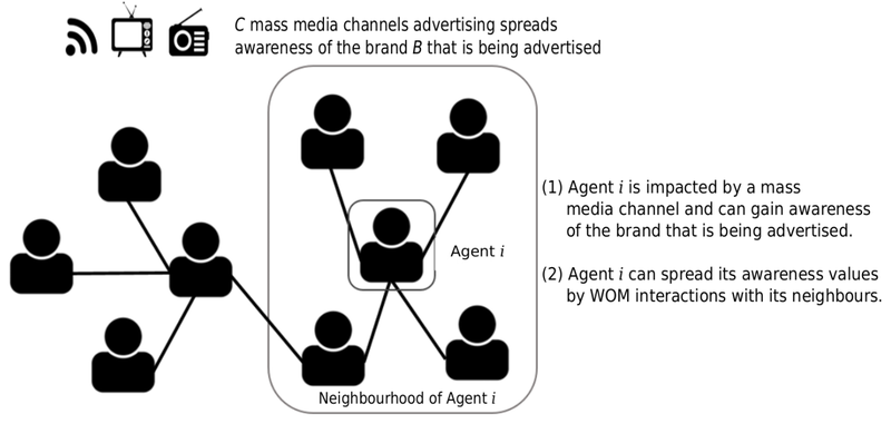
In summary, the ABM attempts to reproduce the impact of social interactions in a particular market and enable brands to influence such interactions via advertising. Next, we detail a set of different parameters that define interactions through multiple agents.
Agent’s state and heuristic rules for decision making
The awareness values of the agents are modeled using a state variable \(a_{i}^{b} \in { 0,1 }\). \(a_{i}^{b}(t) = 1\) represents that agent \(i \in \{1,...,I\}\) is aware of brand \(b \in \{1,...,B\}\) at time step \(t\); while \(a_{i}^{b}(t) = 0\) represents that agent is not aware of brand \(b\). This state variable is initialised using an initial awareness parameter set (\(a^b(0) \in [0,1]\)), which represents the global awareness of the population at the beginning of the simulation, fulfilling \(a^b(0) = \frac{1}{I} \sum_{i=1}^{I} a_{i}^{b}(0)\). Therefore, the percentage of agents with awareness of the different brands at the beginning of the simulation depends on the value of the initial awareness parameter for each brand.
The awareness values of the agents can change at each step of the simulation. On the one hand, agents may gain awareness of a brand due to advertising or due to interacting with other agents through a WOM diffusion process. On the other hand, the awareness of a brand may be lost over time due to a deactivation process (Robles et al. 2020) if it is not reinforced by new stimuli. These losing/gaining effects are modeled with additional parameters, described in the next paragraph.
The parameter regulating the rate at which awareness is lost over time is called awareness deactivation probability (\(d \in [0,1]\)). This process is modeled by checking each brand \(b\) that agent \(i\) is aware of (\(a_{i}^{b}(t) = 1\)) at the start of each step \(t\) and deactivating it with a probability \(d\) by setting \(a_{i}^{b}(t) = 0\). If the deactivation takes effect, the agent could still re-gain awareness due to WOM diffusion and/or the action of mass media channels during the subsequent simulation steps.
In addition to brand awareness, each agent stores the number of conversations produced during its diffusion process. This information is used to compute the WOM volume generated by each brand for the whole population (\(\omega^{b}(t)\)). Every time an agent starts a diffusion process and talks with its neighbourhood, the variable \(\omega_{i}^{b}(t)\) is updated by incrementing it with the total number of conversations, which corresponds to the number of neighbours of the agent.
Underlying social network and word-of-mouth interactions
Agents are connected through an artificial social network (Barabási & Albert 1999; Watts & Strogatz 1998) where each node is an agent and edges represent the connections of the agents with their direct contacts. We model this social network using an artificial scale-free network (Barabási & Albert 1999) with a power-law degree distribution. This means a few nodes have a significantly large number of connections (hubs of the social network) and most nodes have a very low number of connections. Our scale-free network is generated via the Barábasi-Albert preferential attachment algorithm (Barabási & Albert 1999) which uses a parameter \(m\) to regulate the network’s growth rate and its final density.
The agents of the model can spread their awareness values during the simulation through the artificial social network. Interactions between consumers occur during all the simulation steps and facilitate the information diffusion process among the agents (Rogers 2010). Every agent \(i\) has a talking probability \(p(t)_{i}^{b} \in [0,1]\) to spread its awareness at time step \(t\) for every brand \(b\). This probability specifies when the agent \(i\) talks with all of its neighbours in the artificial social network. The contagion effect is modeled using the WOM awareness impact parameter (\(\alpha^{WOM} \in [0, 1]\)), which represents the probability of a neighbour agent \(j\) (direct neighbour of \(i\)) gaining awareness of a brand after having a conversation about it with agent \(i\).
Mass media channels description
We model external influences like brand advertising as global mass media using a similar approach to the one applied in the social network. The external influences are parameterised to define the differences between the channels (i.e. press, radio and television). The mass media channels in \(C\) influence agents randomly depending on the potential of the channel to reach the population and the investment amount of each brand. The maximum population percentage that can be reached by a mass media channel is bounded by the nature of the channel itself. For example, the maximum population percentage that can be reached by a TV ad is bounded by the maximum population percentage that watches TV. We model these different properties with a reach parameter (\(r_{c} \in [0, 1], \forall c \in \{1,...,C\}\)), which limits the maximum number of agents a channel \(c\) is able to hit during a single step.
The advertising campaigns of the mass media channels are modeled using gross rating points (GRPs). In advertising (Farris et al. 2010), a GRP is a measure of the magnitude of the impressions scheduled for a mass media channel. Specifically, we use the convention that one GRP means reaching 1% of the target population. The variable \(\chi_{c}^{b}(t)\) models the investment units in GRPs for channel \(c\) by brand \(b\) and time step \(t\). Each channel has different costs for the invested GRP units, and the brands need to carefully choose their investment since increasing the population awareness or the number of conversations using mass media channels implies a monetary cost (i.e. brands need to define their marketing mix among the existing channels).
Similarly to the way we model social interactions, all the channels \(c \in C\) consider an awareness impact parameter (\(\alpha_{c} \in [0, 1], \forall c \in \{1,...,C\}\)) that models the probability of the agent becoming aware of the brand after one channel impact. Moreover, the effect of the advertising transmitted by mass media channels can produce a viral buzz effect in the reached agent, as done in (Moya et al. 2017). This buzz effect boosts the number of conversations about the announced brand, increasing the talking probability of the reached agents (\(p_{i}^{b}\)). This effect is modeled using a variable called buzz increment (\(\tau_{c}\)) defined for each channel \(c\). The increment produced on agent talking probability is computed as a percentage increment over the initial talking probability of agent \(i\) (\(p_{i}^{b}(0)\)). However, if the generated buzz is not reinforced, its effect could decay over time as previous interactions are forgotten. We use a variable \(d\tau_{c}\), called buzz decay, to reduce previous increments on the talking probability (\(\sigma_c\)). Equation 1 defines the updating process for the talking probability of agent \(i\) for brand \(b\) due to both buzz increment and decay effects of channel \(c\).
| \[\begin{split} p_{i}^{b}(t+1)=p_{i}^{b}(t) + p_{i}^{b}(0) \cdot \tau_{c} - {\sigma_{i}^{b}}_{c}(t) \cdot d\tau_{c}, \\ \mbox{ where } {\sigma_{i}^{b}}_{c}(t) = \sum_{s=1}^{t} (p_{i}^{b}(s) - p_{i}^{b}(0) \cdot \tau_{c}). \end{split} \] | \[(1)\] |
Experimental Design
Problem scenarios
The experimentation considers 12 different instances of an ABM which models a real banking marketing scenario. The dimensionality of each instance directly depends on the number of channels \(|C|\) in the virtual market. It is important to mention that the number of channels in a specific market (regardless of the instances we use in our experimental setup) is variable and depends on the market. Since the method must be generic to be useful in any market, \(|C|\) cannot be a specific number but rather a variable that is defined by the modeller in each market.
The final set of parameters which are selected for calibration is determined by the size of the model instance: three parameters for each mass media channel plus three fixed social parameters. Thus, the number of parameters being calibrated is computed as \((|C| + 1) \cdot 3\). Briefly, these parameters are the following:
- Mass media parameters: For each defined mass media channel \(c \in C\), we calibrate its awareness impact (\(\alpha_{c}\)), buzz increment (\(\tau_c\)) and buzz decay (\(d\tau_c\)).
- Social network parameters: We calibrate the initial talking probability (\(p^{b}(0)\)), social awareness impact (\(\alpha^{WOM}\)) and awareness deactivation (\(d\)).
We have an initial baseline instance, referred to as P1(24) corresponding to a real market with \(|C|=7\) channels, from which the rest of the instances are synthetically generated. The complete set of model parameters corresponding to this baseline instance is collected in Table 1. Each instance variation introduces additional mass media channels that are generated from the initial ones by modifying its investment values.
| Name | Description | Value |
|---|---|---|
| Fixed parameters | ||
| \(|I|\) | Number of agents | 1000 |
| \(|B|\) | Number of brands | 8 |
| \(|C|\) | Number of mass media channels | 7 |
| \(|T|\) | Number of steps | 52 |
| \(m\) | Parameter for social network generator | 4 |
| \(a^b(0)\) | Initial awareness for brand \(b\) | 0.71, 0.76, ... |
| \(r_{c}\) | Reach for mass media channel \(c\) | 0.93, 0.58, ... |
| Parameters to calibrate | ||
| \(d\) | Awareness deactivation probability | - |
| \(p_{i}^{b}(0)\) | Initial talking probability, same value for each brand \(b\) | - |
| \(\alpha^{WOM}\) | Awareness impact for social interactions | - |
| \(\alpha_{c}\) | Awareness impact for mass media channel \(c\) | - |
| \(\tau_{c}\) | Buzz increment for mass media channel \(c\) | - |
| \(d\tau_{c}\) | Buzz decay for mass media channel \(c\) | - |
In addition, each model includes a random perturbation of the target historical values for both KPIs, awareness and WOM volume. Each of the newly generated instances increases the dimensionality of the previous one, including new decision variables to enable a more complete comparison of the different MMEAs, as seen in Table 2. Note that each instance is labeled using its number of decision variables: P1(24), P2(39), P3(45), P4(54), P5(60), P6(69), P7(75), P8(84), P9(90), P10(99), P11(114) and P12(129).
| Instance | P1 | P2 | P3 | P4 | P5 | P6 | P7 | P8 | P9 | P10 | P11 | P12 |
|---|---|---|---|---|---|---|---|---|---|---|---|---|
| Channels (\(|C|\)) | 7 | 12 | 14 | 17 | 19 | 22 | 24 | 27 | 29 | 32 | 37 | 42 |
| Decision variables | 24 | 39 | 45 | 54 | 60 | 69 | 75 | 84 | 90 | 99 | 114 | 129 |
Variations on the existing mass media channels \(C\) consist in either increasing or reducing the original investment of each brand for each of its steps, multiplying its value by a given factor. We consider reduction factors for the original values of 15%, 30%, 45% and 60%, and increasing factors of 100%, 200%, 300%, and 400%. The latter decisions are taken at random and remain unchanged for each step. In contrast, modifications to the target values of awareness and WOM volume are applied adding or subtracting a given quantity to each of its time steps. In this way, each modification to the target awareness values adds or subtracts 2%, 5%, 8% or 10% to/from the target brand values. The resulting awareness values are truncated between 1% and 100% to avoid unrealistic target values. With respect to target WOM volume, each increasing or decreasing modification is of either 1,000, 2,000, 4,000 or 6,000 conversations, keeping the conversation values above 0. Table 3 shows an example of the process carried out to generate the instances.
| P2(40) | |||||||||
|---|---|---|---|---|---|---|---|---|---|
| New channels generation | |||||||||
| Original channel | New channel | b1 | b2 | b3 | b4 | b5 | b6 | b7 | b8 |
| 3 | 8 | +100% | -15% | -15% | -45% | +200 | -60% | +300% | -30% |
| 5 | 9 | +100% | -30% | +400% | +200% | +300% | -30% | -30% | -15% |
| 5 | 10 | -15% | -15% | +300% | +300% | +200% | -30% | +300% | -30% |
| 3 | 11 | -60% | +100% | +300% | -45% | +200% | +400% | -45% | -15% |
| 6 | 12 | +200% | -15% | -60% | -30% | -30% | +400% | -60% | 200% |
| Target awareness modification | |||||||||
| b1 | b2 | b3 | b4 | b5 | b6 | b7 | b8 | ||
| -10% | -8% | +10% | +10% | -8% | -5% | +5% | +5% | ||
| Target WOM volume modification (Conversations) | |||||||||
| b1 | b2 | b3 | b4 | b5 | b6 | b7 | b8 | ||
| -6,000 | -6,000 | -4,000 | +4,000 | +6,000 | -2,000 | +4,000 | -1,000 | ||
Calibration parameters
From Table 1, we select for automatic calibration the parameters that control either the dynamics of agent awareness values or the number of conversations the agent holds, as these are the most uncertain and the hardest to estimate by the modeller using the available data (Moya et al. 2019). Table 4 summarises the parameter values of the baseline instance. The remaining instances share this initial setup, along with the corresponding reach parameter value \(r_{c}\) for any new mass media channel which takes the value of the original channel employed in its generation. That is, if a new mass media channel \(c_{12}\) is generated using the original channel \(c_3\) it shares the reach parameter value (i.e. \(r_{12}=r_{3}\)).
| Baseline instance P1(24) | |||||||
|---|---|---|---|---|---|---|---|
| Name | Value | Name | Value | Name | Value | Name | Value |
| \(a^{b_1}(0)\) | 0.71 | \(a^{b_2}(0)\) | 0.76 | \(a^{b_3}(0)\) | 0.59 | \(a^{b_4}(0)\) | 0.26 |
| \(a^{b_5}(0)\) | 0.08 | \(a^{b_6}(0)\) | 0.43 | \(a^{b_7}(0)\) | 0.4 | \(a^{b_8}(0)\) | 0.34 |
| \(r_{1}\) | 0.93 | \(r_{2}\) | 0.58 | \(r_{3}\) | 0.55 | \(r_{4}\) | 0.04 |
| \(r_{5}\) | 0.43 | \(r_{6}\) | 0.38 | \(r_{7}\) | 0.7 | \(p^{b}(0)\) | 0.1 |
The calibration process assigns each of the selected model parameters to a single decision variable, limiting the range of possible parameter values to a real-coded \([0, 1]\). Table 5 shows an example of a tentative calibration solution for instance P2(39).
| \(\alpha_{1}\) | \(\alpha_{2}\) | \(\alpha_{3}\) | \(\alpha_{4}\) | \(\alpha_{5}\) | \(\alpha_{6}\) | \(\alpha_{7}\) |
|---|---|---|---|---|---|---|
| 4.420592e-05 | 0.9275268 | 0.91726940 | 0.358706832 | 1.991031e-04 | 0.188117322 | 7.712790e-03 |
| \(\tau_{1}\) | \(\tau_{2}\) | \(\tau_{3}\) | \(\tau_{4}\) | \(\tau_{5}\) | \(\tau_{6}\) | \(\tau_{7}\) |
| 0.919016368 | 0.85484480 | 0.445861067 | 0.037229668 | 0.42503753 | 0.7193559683 | 0.046021892 |
| \(d\tau_{1}\) | \(d\tau_{2}\) | \(d\tau_{3}\) | \(d\tau_{4}\) | \(d\tau_{5}\) | \(d\tau_{6}\) | \(d\tau_{7}\) |
| 0.013241515 | 0.19740914 | 0.4053775552 | 0.008095596 | 0.670678402 | 0.803071854 | 0.463061986 |
| \(p^{b}\) | \(\alpha^{WOM}\) | d | \(\alpha_{8}\) | \(\tau_{8}\) | \(d\tau_{8}\) | |
| 0.1287573 | 0.02508721 | 0.06805826 | 0.780366135 | 0.134720552 | 0.6739496654 | |
| \(\alpha_{9}\) | \(\tau_{9}\) | \(d\tau_{9}\) | \(\alpha_{10}\) | \(\tau_{10}\) | \(d\tau_{10}\) | |
| 0.8341758 | 0.004248453 | 0.737444678 | 0.6065266 | 0.80506945 | 0.226626727 | |
| \(\alpha_{11}\) | \(\tau_{11}\) | \(d\tau_{11}\) | \(\alpha_{12}\) | \(\tau_{12}\) | \(d\tau_{12}\) | Fitness |
| 0.790572098 | 0.128404770 | 0.739637188 | 0.0015857279 | 0.7423187907 | 0.831388290 | 38.15518 |
Fitness functions
Equations 2 and 3 define the mean absolute percentage error (MAPE) functions, \(f_{1}\) and \(f_{2}\), that compare the historical data with respect to the simulation outputs during each evaluation of a candidate solution.
| \[f_{1} = \frac{100}{T \cdot B}\sum_{b=1}^{B}\sum_{t=1}^{T} \left | \frac{ a^b(t) - \widetilde{a}^b(t)}{ \widetilde{a}^b(t) } \right |, \] | \[(2)\] |
| \[f_{2} = \frac{100}{T \cdot B}\sum_{b=1}^{B} \sum_{t=1}^{T} \left | \frac{\omega^b(t) - \widetilde{\omega}^b(t) }{ \widetilde{\omega}^b(t) } \right |, \] | \[(3)\] |
The simulated values are generated by running several Monte-Carlo simulations of the ABM considering the parameter setup encoded in the evaluated solution and by computing the average of those independent runs. \(f_{1}\) and \(f_{2}\) are combined in a final objective function \(f\) as follows:
| \[f = \frac{1}{R} \sum_{i=1}^{R} \beta f_{1}^{i} + (1-\beta) f_{2}^{i}, \] | \[(4)\] |
Experimental setup
We run each MMEA 20 independent times using different random seeds. In order to adapt the algorithms to the problem size and to the dimensionality of its search space, we define a variable population size \(P = 10 \cdot D\), where \(D\) is the number of variables being calibrated. Furthermore, we set as algorithm stopping criterion a number of evaluations proportional to the problem dimension by multiplying \(P\) by \(50\) for each problem instance. The fitness of the individual is calculated as the average value of \(f\) for \(R=15\) Monte-Carlo simulations of the ABM, which proved to be sufficient in a previous experimentation. A weight \(\beta = 0.5\) is considered in the objective function.
All the selected MMEAs are implemented in Java using the ECJ framework (Luke 1998). The initial populations of the MMEAs are randomly initialised and follow a real coding scheme. The hyperparameter setup for the MMEAs was defined via an extensive preliminary experimentation in which every algorithm was run with a different set of hyperparameter values. We tested the algorithms starting with the configurations their authors recommend in the literature and then extended these values by using minimum and maximum ranges. Finally, we selected from the entire range of values those hyperparameter configurations which performed best, obtaining a reference for each algorithm with the following final values:
- Traditional niching methods: We set the distance radius \(\sigma_{share}\) to \(0.033\) for both Sharing and Crowding. The generation gap (\(G\)) and the crowding factor (\(CF\)) are set to 3 for the Crowding method. Finally, we set a niche capacity \(k=3\) for Clearing. The three methods use the same selection, crossover and mutation operators: a ternary tournament selection method, a BLX-\(\alpha\) crossover operator with \(\alpha=0.6\) and crossover probability \(p_{c}=0.3\), and a random mutation operator applied to each individual with a probability \(p_{m}=0.25\).
- Niching methods based on DE: As these are all parameterless/adaptive methods, there is no need to set any parameters for the niching mechanisms. The value for the crossover rate is set to \(CR=0.9\) for all the methods, while the mutation rate is set to \(F=0.5\) for SHADE, L-SHADE and DE/nrand/2, and to \(F=0.8\) for MOBiDE. For both SHADE and L-SHADE, we set the size of the historical memory to the dimensionality of the model being calibrated, \(D\). The \(N_{init}\) and the \(N_{min}\) for the L-SHADE method are set to \(P\) and 4, respectively.
- NichePSO: We set the maximum allowed radius to \(R_{max}=0.1\) and the values for \(\delta\) and \(\mu\) to \(-10^{-4}\) and \(-10^{-3}\), respectively.
- PNA-NSGA-II: As an adaptative method, it is not necessary to set the niching mechanism parameters. We define the number of objectives in which the original objective needs to be decomposed to 2 to use the NSGA-II method. Then we use the same parameter configuration as in (Bandaru & Deb 2013), also using a simulated binary crossover (SBX) (Deb & Agrawal 1995) for continuous search space.
Results
We first define the evaluation criteria and solution filtering used during the analysis of the experiments. Then, we analyse and compare the performances of the different MMEAs, showing the different solutions obtained by the best-performing MMEA in the decision space and, finally, we analyse how the fitness distributions change between some problem instances.
We consider three different measures to evaluate and rank the best calibration solutions across the different model scenarios: efficacy (the calibration error defined in Equation 4), multi-solution based efficacy (capability to find multiple optima) and diversity in the final set of solutions. This performance assessment checks if the calibration algorithm explores well when optima belong to different regions and exploits well a region where there are similar optimal solutions. We compare the calibration performance of the different MMEAs by ranking them in terms of fitness performance (i.e. model fitting) by considering the average fitness values of the set of solutions returned by the MMEAs. Additionally, we perform statistical tests on the different results and use visualization tools such as heat maps to visualise the search space of the parameters and place the set of solutions returned by the MMEAs in them to illustrate the model validation capabilities of multimodal calibration.
Comparing MMEA performances
Table 6 shows the average, standard deviation and minimum fitness values obtained by the MMEAs over the 12 instances. The last column of Table 6 shows the minimum and maximum average fitness obtained for each instance. In Table 7 we complement the latter information with a statistical test considering the ranking of the algorithms and apply several post-hoc procedures to highlight significant differences in their performance. We perform Friedman’s non-parametric test, Bonferroni-Dunn’s test, and Holm’s test. The average ranking and the resulting \(p-\)values of Bonferroni-Dunn’s test and Holm’s test are shown in Table 7.
The values in Table 6 show that SHADE is the best performing algorithm with a a mean rank of 1.33. SHADE obtains the lowest (closest to the historical data) average fitness values in 9 of the 12 model instances, while achieving the minimum fitness value for all instances. L-SHADE is the second best performing algorithm with a mean rank of 3, achieving the best average fitness value in the P3 and P12 model instances. With a low difference with respect to L-SHADE, NichePSO is the third best MMEA with a mean rank of 3.08. NichePSO achieves the best average fitness value in the P7 model instance and the second best average fitness in 5 of the 12 model instances, while also being the second ranked algorithm in terms of minimum fitness (7 out of the 12 instances). PNA-NSGA-II is in fourth position in terms of average fitness with a mean rank of 3.58, while MOBiDE obtains the fifth position of the five best performing MMEAs with a mean rank of 4. In contrast, Crowding, Sharing, DE/nrand/2 and Clearing, with respective mean ranks of 6, 7.17, 8 and 8.83, show the poorest performance, between 1.1% and 1.6% worse than the best algorithm.
Although some distance behind the five best-performing algorithms, the Crowding GA is the best performing classical MMEA, obtaining better results than a more recent method such as DE/nrand/2. The results show that, although the dimension of the problem is increased with each instance of the model, SHADE continues to provide the best performance. This makes SHADE independent of the dimensionality of the calibration problem and suggests it would be a suitable method for the calibration of high dimensional ABM instances.
| SHADE | L-SHADE | NichePSO | PNA-NSGA-II | MOBiDE | Crowding GA | Sharing GA | DE/nrand/2 | Clearing GA | Fitness Value [min., max.] | ||
| P1 | \(\bar{x}\) (\(Std\)) | 27.14 (1.53) | 29.07 (1.11) | 28.27 (1.09) | 29.52 (2.38) | 28.82 (2.08) | 32.58 (0.39) | 33.53 (0.57) | 33.53 (0.59) | 33.65 (0.41) | [27.14, 33.65] |
| \(best\) | 25.27 | 26.66 | 27.41 | 25.37 | 26.51 | 31.61 | 32.24 | 32.12 | 32.99 | ||
| P2 | \(\bar{x}\) (\(Std\)) | 38.43 (0.19) | 39.13 (0.36) | 43.95 (2.43) | 38.66 (0.27) | 39.97 (0.86) | 50.82 (0.82) | 52.58 (1.24) | 52.37 (1.68) | 53.05 (0.59) | [38.43, 53.05] |
| \(best\) | 38.16 | 38.67 | 39.11 | 38.21 | 38.87 | 49.12 | 49.60 | 47.39 | 51.98 | ||
| P3 | \(\bar{x}\) (\(Std\)) | 26.78 (2.83) | 25.69 (0.47) | 28.76 (1.5) | 26.74 (0.86) | 27.49 (1.02) | 28.86 (0.28) | 30.11 (0.5) | 30.75 (0.82) | 30.3 (0.3) | [25.69, 30.3] |
| \(best\) | 22.92 | 24.87 | 24.65 | 25.12 | 25.13 | 28.28 | 28.48 | 29.24 | 29.61 | ||
| P4 | \(\bar{x}\) (\(Std\)) | 31.21 (1.7) | 34.78 (1.64) | 34.2 (2.8) | 35.78 (2.38) | 32.70 (0.47) | 38.39 (0.25) | 40.28 (0.43) | 42.5 (0.51) | 41.79 (0.58) | [31.21, 42.5] |
| \(best\) | 29.52 | 32.19 | 31.63 | 31.21 | 31.99 | 37.61 | 39.52 | 41.55 | 40.68 | ||
| P5 | \(\bar{x}\) (\(Std\)) | 28.02 (1.34) | 29.67 (0.40) | 29.96 (2.5) | 29.55 (1.49) | 28.73 (1.43) | 33.26 (0.18) | 35.6 (0.33) | 37.16 (0.54) | 37.21 (0.51) | [28.02, 37.21] |
| \(best\) | 25.69 | 28.50 | 26.07 | 27.07 | 27.31 | 32.69 | 34.96 | 36.19 | 35.96 | ||
| P6 | \(\bar{x}\) (\(Std\)) | 40.44 (0.67) | 41.01 (0.09) | 40.87 (1.54) | 41.91 (0.30) | 43.88 (1.75) | 45.48 (0.34) | 51.98 (0.71) | 54.59 (0.70) | 55.4 (0.82) | [40.44, 55.4] |
| \(best\) | 39.22 | 40.84 | 39.71 | 41.35 | 40.69 | 44.93 | 50.6 | 52.67 | 53.62 | ||
| P7 | \(\bar{x}\) (\(Std\)) | 35.63 (0.92) | 38.16 (1.23) | 35.25 (1.72) | 36.78 (1.94) | 36.77 (1.28) | 42 (0.22) | 45.04 (0.28) | 45.93 (0.43) | 46.59 (0.42) | [35.25, 46.59] |
| \(best\) | 33.82 | 35.54 | 34.06 | 34.31 | 34.92 | 41.64 | 44.45 | 45.19 | 46.02 | ||
| P8 | \(\bar{x}\) (\(Std\)) | 29.42 (1.73) | 32.79 (1.40) | 32.2 (1.59) | 34.37 (1.25) | 37.48 (0.64) | 48.20 (0.38) | 53.27 (0.47) | 54.35 (0.58) | 55.86 (0.74) | [29.42, 55.86] |
| \(best\) | 26.23 | 31.39 | 29.47 | 32.32 | 34.89 | 46.91 | 52 | 52.68 | 54.52 | ||
| P9 | \(\bar{x}\) (\(Std\)) | 25.53 (0.85) | 29.30 (0.62) | 28.04 (1.73) | 29.54 (2.17) | 30.85 (0.62) | 40.32 (0.36) | 46.76 (0.66) | 48.37 (0.63) | 49.49 (0.45) | [25.53, 49.49] |
| \(best\) | 24.34 | 27.66 | 25.18 | 25.87 | 29.92 | 39.55 | 45.27 | 46.44 | 48.74 | ||
| P10 | \(\bar{x}\) (\(Std\)) | 43.97 (1.3) | 44.99 (0.82) | 47.85 (2.11) | 47.30 (0.56) | 50.25 (3.20) | 53.91 (0.27) | 67.62 (1.32) | 70.16 (1.21) | 73.46 (1.47) | [43.97, 73.46] |
| \(best\) | 41.69 | 43.39 | 43.98 | 46.31 | 44.79 | 53.45 | 64.15 | 68.52 | 70.41 | ||
| P11 | \(\bar{x}\) (\(Std\)) | 27.69 (1.25) | 30.22 (0.57) | 28.43 (0.89) | 32.5 (1.54) | 32.87 (1.36) | 42.64 (0.35) | 47.04 (0.43) | 47.64 (0.68) | 48.57 (0.32) | [27.69, 48.57] |
| \(best\) | 25.36 | 29.09 | 26.31 | 28.69 | 29.5 | 41.85 | 46.26 | 46.05 | 47.85 | ||
| P12 | \(\bar{x}\) (\(Std\)) | 28.78 (3.70) | 27.38 (0.22) | 32.18 (1.74) | 29.64 (0.46) | 32.59 (1.52) | 36.93 (0.45) | 40.73 (0.36) | 41.37 (0.44) | 42.06 (0.60) | [27.38, 42.06] |
| \(best\) | 26.36 | 27.07 | 27.93 | 29 | 29.89 | 35.97 | 39.98 | 40.56 | 40.05 | ||
On the basis of the above analysis, we can clearly divide the MMEAs into two groups based on their performance. On the one hand we have the three classical MMEAs (Crowding, Clearing, and Sharing) as well as DE/nrand/2. On the other, we have SHADE, L-SHADE, MOBiDE, NichePSO and PNA-NSGA-II as the most accurate MMEAs.
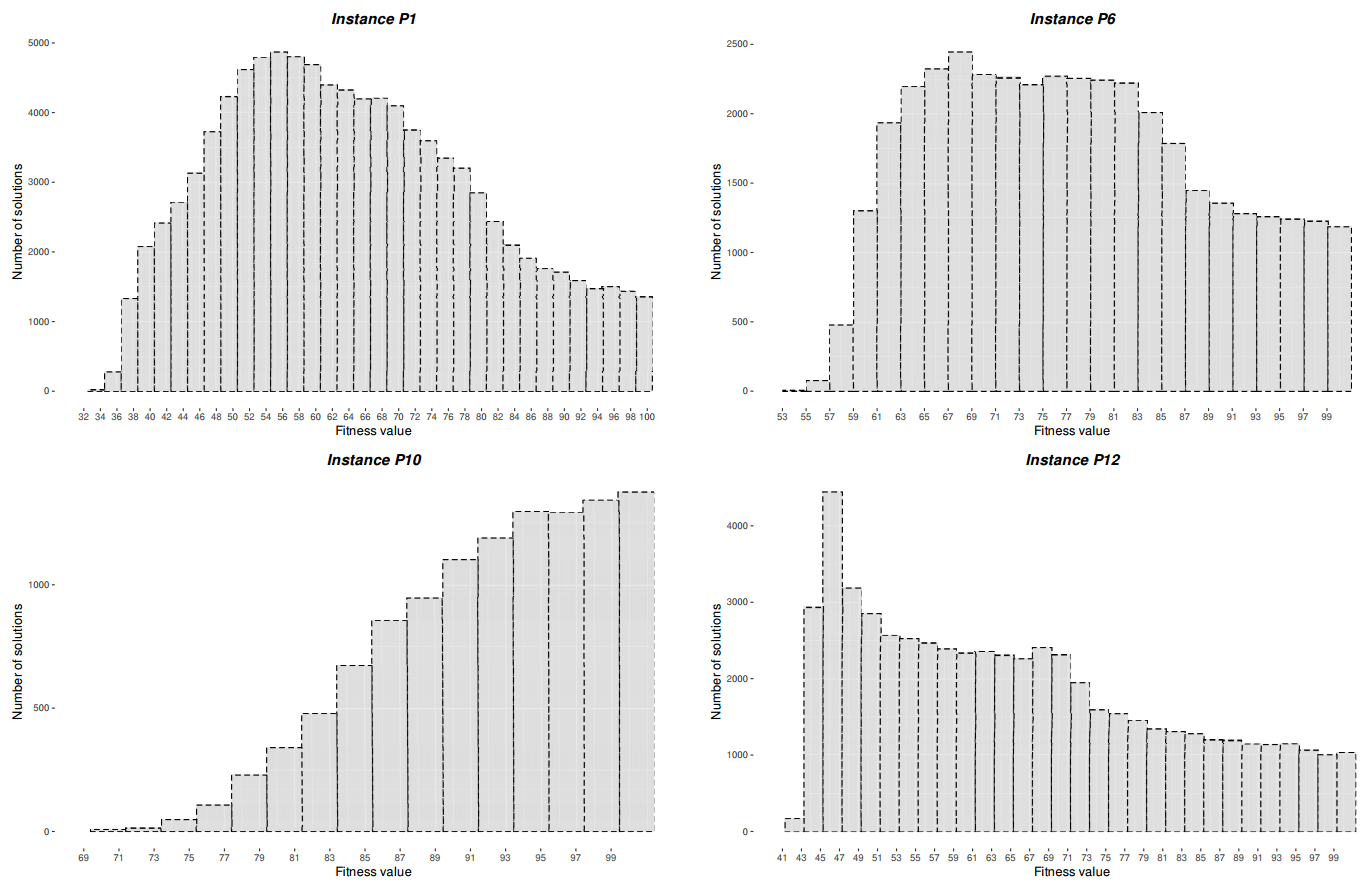
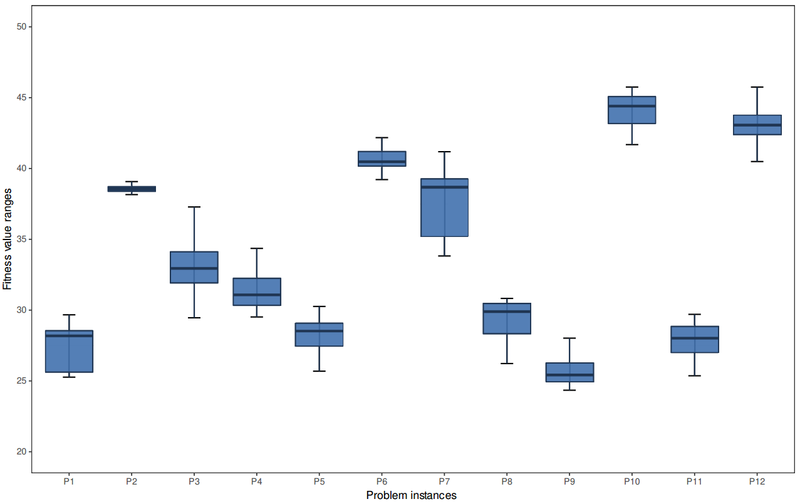
Moreover, we can draw two interesting conclusions from the values in Table 6. First, we can observe that the differences in accuracy between the worst and best algorithms gradually increase with the dimensions of the model. Thus, we can see in the last column of Table 6 that these differences are closer from P1 to P7 (around 20%) than from P8 to P12, where the performance of the worst algorithm is around 47% worse than the best algorithm’s value. Therefore, we can affirm that the best algorithms are more suitable for high dimensional ABM instances. The second conclusion comes from the analysis of the differences between the mean, standard deviation and the single best values found for each problem instance. The results obtained by each algorithm change for each instance. Thus, although the same virtual market (P1) is used to generate the problem instances, both the search space dimension and the market dynamics change from one instance to another, resulting in different behaviours from the ABM instances (in fact, they comprise virtual markets with different characteristics and complexities). We generated and evaluated 200,000 random solutions to build the fitness histograms shown in Figure 2 as an illustrative example of how the fitness distributions change among different problem instances. Figure 3 then shows how the fitness ranges of the solutions obtained by SHADE in the calibration process also change from one problem instance to another. The two figures demonstrate the potential of the best-performing algorithms to keep finding promising parameter configurations while the dimension and complexity of the market dynamics increase.
Finally, Table 7 presents the corresponding average ranking and the resulting \(p\)-values of Bonferroni-Dunn’s and Holm’s tests using SHADE as the control method. With respect to Friedman’s test, the result of applying the test is \(\chi^2_F = 85.62\) and its corresponding \(p-\)value is \(3.59 \cdot 10^{-5}\), which is lower than the desired level of significance (\(\alpha = 0.01\)), with the conclusion that there are significant differences between the performance of the algorithms.
| Rank | Bonferroni \(p\) | Holm \(p\) | |
|---|---|---|---|
| SHADE | 1.33 | \(-\) | \(-\) |
| L-SHADE | 3 | 0.92 | 0.2 |
| NichePSO | 3.08 | 0.79 | 0.2 |
| PNA-NSGA-II | 3.58 | 0.27 | 0.1 |
| MOBiDE | 4 | 0.09 | 0.05 |
| Crowding GA | 6 | \(<10^{-5}\) | \(<10^{-5}\) |
| Sharing GA | 7.17 | \(<10^{-7}\) | \(<10^{-7}\) |
| DE/nrand/2 | 8 | \(<10^{-9}\) | \(<10^{-9}\) |
| Clearing GA | 8.83 | \(<10^{-11}\) | \(<10^{-11}\) |
Considering the rank positions in Table 7, we can verify the dominance of SHADE as it outperforms all other methods in terms of the minimum fitness value obtained and achieves the most robust behaviour in 9 of the 12 instances in terms of averaged fitness values.
Analysis of the best calibration results
Here we show how the algorithm performs when exploring the parameter space of some of the 12 model instances calibrated in this contribution. We use heat maps obtained from pairs of calibrated model variables as a tool to better explain SHADE’s performance and to compare it against the third best-performing MMEA (NichePSO) and one of the worst performing (Crowding GA). Although both L-SHADE and NichePSO scored a similar ranking position, we choose NichePSO for the visual comparison as L-SHADE is an extension of the best method (SHADE) and offered similar solutions. We conclude the section reporting the parameter configuration which SHADE obtains for some problem instances (i.e. the calibrated parameters for some of the ABMs of different virtual markets).
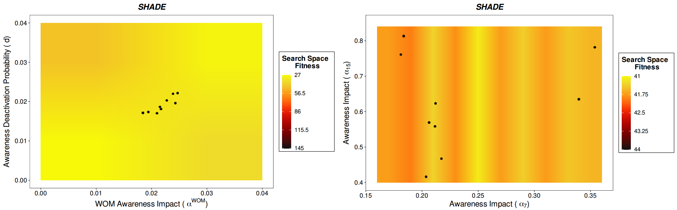
Figures 4 and 5 show the set of solutions obtained by SHADE, NichePSO, and Crowding in the calibration of the P1 and P6 instances. Both Figures 4 and 5 are projections on two variables of all the variables to be calibrated (minimum 24). The plots in the first row of Figure 4 represent the awareness impact (X axis) and the awareness deactivation probability parameter values (Y axis) for SHADE and NichePSO, while the plot in the second row represents the same values for Crowding GA. Figure 5 represents the awareness impact in media channel 7 (X axis) and the awareness impact in channel 15 (Y axis). In both cases, the black circles represent the best calibrated models in terms of historical fitting. Finally, Figure 6 shows a close-up view of the solutions obtained by SHADE, the best performing MMEA, using the same parameter combination as in Figures 4 and 5 to better appreciate their diversity in the problem search space.
It should be noted that these figures were built using the best result obtained in the 20 runs defined for each algorithm in the experimental setup and that the exact configuration of the search space for the addressed problem is unknown. Moreover, the distribution of the optimal solution is only approximated in the heat maps by the best solution found so far as a way to interpret the results. Thus, the color gradient displayed in Figures 4 and 5 shows different search space landscapes depending on the combination of the two parameters considered. These plots represent simple relationships between 2 variables which comprise very limited approximations to the complex relations existing in the multidimensional search space. Moreover, both Figures 4 and 5 are partial representations of the whole search space landscape, since they relate the search space and the target space only for two of the minimum of 24 variables that are in the problem. Even so, we think these figures provide interesting and easily comprehensible insights into the problem being tackled. Our aim is to visualise the dispersion of the solutions provided by each algorithm and, at the same time, to evaluate their fitness to corroborate the algorithm’s performance.
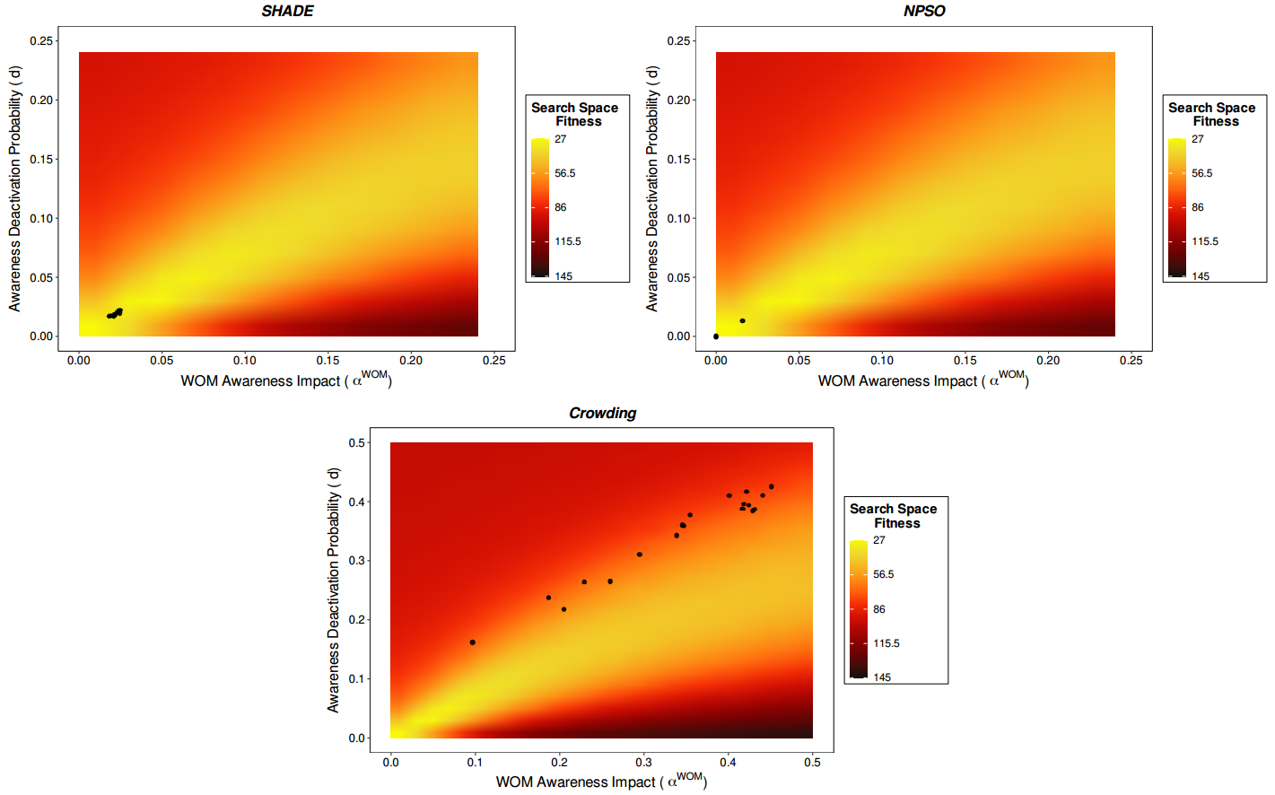
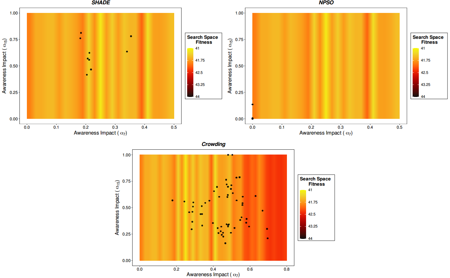
Although the set of SHADE solutions does not seem to cover the search space as the NichePSO does, it is nonetheless able to explore the most promising regions (see Figure 6), finding the best parameter configurations even if the search space has a high complexity at a smaller scale. Moreover, SHADE keeps on showing a good search space exploration and exploitation in high dimensional instances of the ABM, as seen for example in the P6 instance in Figure 5, whereas NichePSO starts reducing its performance, unable to find optimal solutions or locate solutions in the best regions of the search space.
The Crowding GA shows a poor performance in both the P1 and P6 instances. Although it seems to deliver more diverse solutions in both instances, it is unable to find high quality local or global solutions, or to focus on a near region of the search space and look there for high quality optimal solutions. Figures 4 and 5 show how the exploration of the search space performed by Crowding is some distance from the regions where the most promising parameter configurations are located.
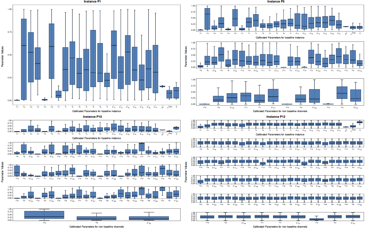
Although SHADE has a better dispersion balance compared to NichePSO and Crowding GA, it does not cover all the optimal search space available for the parameter combinations analysed in Figures 4 and 5. One reason for this behaviour could be the existence of some unknown factors that limit the range of good solutions. However, it is important to note that we are showing only two two-parameter relationships from a large set of calibration parameters and that multidimensional relationships can be much more complex and have bias in particular parameter pairs. Thus, we cannot confirm that the SHADE coverage of the optimal search space behaves similarly for all the parameter combinations of all the problem instances considered in this work. The high dimensionality of the model being analysed and the lack of space in the manuscript makes it unfeasible to show every parameter combination. Instead, we include Figure 7 to observe the distributions of the values for each calibration parameter that the best MMA finds for different instances of the problem. As in Figures 4 and 5, the parameter distributions shown in Figure 7 result from grouping the best solutions from the 20 independent runs for each instance of the problem.
Figure 7 allows us to understand how the parameter combinations change as the size of the instances increases. As can be seen, from the base instance (upper left corner) to the largest instance (lower right corner), the value ranges for parameters such as \(\alpha^{WOM}\), \(d\), \(\alpha_{c}\) or \(\tau_{c}\) change for each mass media channel. On the one hand, this phenomenon shows that the algorithm is able to maintain a good performance despite the increase in the complexity and size of the search space. On the other, it also illustrates that changes in the model’s structure directly affect the relationships between the parameters being calibrated, making both the parameters and the algorithms involved in the calibration process depend on the problem context (Carrella 2021).
Main Conclusions and Further Research
In this study, a comparative analysis is undertaken of both traditional and recent high-performing MMEAs when calibrating the awareness and word-of-mouth parameters of an ABM. We applied 9 different MMEAs (the Sharing, Crowding and Clearing multimodal extensions of GAs; the SHADE, L-SHADE, DE/nrand/2 and MOBiDE multimodal extensions of DE, NichePSO, a multimodal extension of particle swarm optimisation, and the PNA-NSGA-II extension of NSGA-II) to fit the simulation outputs of an ABM to its real historical data.
Our experimentation comprised 12 instances in which the dimension of the model is gradually increased by incorporating additional channels to the virtual market. Thus, the MMEAs successively tackled the calibration of 24 parameters in the initial instance and 129 parameters in the final instance. We compared the average and minimum fitness values obtained by the selected MMEAs and ranked the best five. Finally, we used heat maps to analyse the decision space and the solutions returned by the two best-performing algorithms.
Some important highlights of our work are:
- The five best ranked algorithms achieved high quality solutions regardless of the dimensionality of the instance being calibrated.
- SHADE outperformed every other considered MMEA, being the best performing algorithm in almost all the experimentation instances.
- SHADE was able to locate and focus on promising regions of the search space, finding the best optimal and global solutions in scenarios with different dimensionality and complexity in a single run.
- MMEAs perform well for ABM calibration when the modeller wants to find diverse parameter configuration problems through a complex and multidimensional search space.
Although five of the nine MMEAs considered performed well when calibrating ABM instances with different dimensionalities and complexities, the results obtained are specific and context-dependent on the analyzed instances (Carrella 2021). Thus, we cannot generalise or assume SHADE is the best performing algorithm for non-tested instances or other ABMs as a consequence of the No Free Lunch theorem (Wolpert & Macready 1997).
The study demonstrates the important capabilities of MMEAs in the exploration of complex multidimensional search spaces such as those handled for ABM calibration, allowing diverse and optimal parameter configurations to be found. Nevertheless, as it is a hard task to select the best parameter configurations from high dimensional problems it could be interesting to use some quantitative and qualitative tools to help modellers when selecting parameter configurations from the final set of solutions. Future works could extensively explore the parameter space to detect possible changes in the dynamics of our ABM in order to test the benefits of using MMEAs and enhance the validation of our results (Fagiolo et al. 2019).
Acknowledgements
This work was supported by the Spanish Ministry of Science, Innovation and Universities, the Andalusian Government, the University of Granada, the Spanish National Agency of Research (AEI), and European Regional Development Funds (ERDF) under grants EXASOCO (PGC2018-101216-B-I00), AIMAR (A-TIC-284-UGR18), and SIMARK (PY18-4475).References
BACK, T. (1996). Evolutionary Algorithms in Theory and Practice: Evolution Strategies, Evolutionary Programming, Genetic Algorithms. Oxford: Oxford University Press.
BADHAM, J., Jansen, C., Shardlow, N., & French, T. (2017). Calibrating with multiple criteria: A demonstration of dominance. Journal of Artificial Societies and Social Simulation, 20(2), 11: https://www.jasss.org/20/2/11.html. [doi:10.18564/jasss.3212]
BANDARU, S., & Deb, K. (2013). A parameterless-niching-assisted bi-objective approach to multimodal optimization. 2013 IEEE Congress on Evolutionary Computation. [doi:10.1109/cec.2013.6557558]
BARABÁSI, A. L., & Albert, R. (1999). Emergence of scaling in random networks. Science, 286(5439), 509–512.
BASAK, A., Das, S., & Tan, K. C. (2012). Multimodal optimization using a biobjective differential evolution algorithm enhanced with mean distance-based selection. IEEE Transactions on Evolutionary Computation, 17(5), 666–685. [doi:10.1109/tevc.2012.2231685]
BERGH, F. van den, & Engelbrecht, A. P. (2002). A new locally convergent particle swarm optimiser. IEEE International Conference on Systems, Man and Cybernetics.
BRITS, R., Engelbrecht, A. P., & Van den Bergh, F. (2002). A niching particle swarm optimizer. Proceedings of the 4th Asia-Pacific Conference on Simulated Evolution and Learning.
CARRELLA, E. (2021). No free lunch when estimating simulation parameters. Journal of Artificial Societies and Social Simulation, 24(2), 7: https://www.jasss.org/24/2/7.html. [doi:10.18564/jasss.4572]
CARRELLA, E., Bailey, R., & Madsen, J. K. (2020). Calibrating agent-Based models with linear regressions. Journal of Artificial Societies and Social Simulation, 23(1), 7: https://www.jasss.org/23/1/7.html. [doi:10.18564/jasss.4150]
CHICA, M., Barranquero, J., Kajdanowicz, T., Cordón, O., & Damas, S. (2017). Multimodal optimization: An effective framework for model calibration. Information Sciences, 375, 79–97. [doi:10.1016/j.ins.2016.09.048]
CHICA, M., Chiong, R., Kirley, M., & Ishibuchi, H. (2018). A networked N-player trust game and its evolutionary dynamics. IEEE Transactions on Evolutionary Computation, 22(6), 866–878. [doi:10.1109/tevc.2017.2769081]
CHICA, M., & Rand, W. (2017). Building agent-based decision support systems for word-of-mouth programs. A freemium application. Journal of Marketing Research, 54(5), 752–767. [doi:10.1509/jmr.15.0443]
DAI, C., Yao, M., Xie, Z., Chen, C., & Liu, J. (2009). Parameter optimization for growth model of greenhouse crop using genetic algorithms. Applied Soft Computing, 9(1), 13–19. [doi:10.1016/j.asoc.2008.02.002]
DAS, S., Maity, S., Qu, B. Y., & Suganthan, P. N. (2011). Real-parameter evolutionary multimodal optimization - A survey of the state-of-the-art. Swarm and Evolutionary Computation, 1(2), 71–88. [doi:10.1016/j.swevo.2011.05.005]
DAS, S., & Suganthan, P. N. (2010). Differential evolution: A survey of the state-of-the-art. IEEE Transactions on Evolutionary Computation, 15(1), 4–31.
DEB, K., & Agrawal, R. B. (1995). Simulated binary crossover for continuous search space. Complex Systems, 9(2), 115–148.
DEB, K., Pratap, A., Agarwal, S., & Meyarivan, T. (2002). A fast and elitist multiobjective genetic algorithm: NSGA-II. IEEE Transactions on Evolutionary Computation, 6(2), 182–197. [doi:10.1109/4235.996017]
DE JONG, K. A. (1975). Analysis of the behavior of a class of genetic adaptive systems.
EPITROPAKIS, M. G., Plagianakos, V. P., & Vrahatis, M. N. (2011). Finding multiple global optima exploiting differential evolution’s niching capability. 2011 IEEE Symposium on Differential Evolution (SDE). [doi:10.1109/sde.2011.5952058]
FAGIOLO, G., Guerini, M., Lamperti, F., Moneta, A., & Roventini, A. (2019). 'Validation of agent-based models in economics and finance.' In C. Beisbart & N. J. Saam (Eds.), Computer Simulation Validation (pp. 763–787). Berlin, Heidelberg: Springer. [doi:10.1007/978-3-319-70766-2_31]
FARRIS, P. W., Bendle, N. T., Pfeifer, P. E., & Reibstein, D. J. (2010). Marketing Metrics: The Definitive Guide to Measuring Marketing Performance. Philadelphia, PA: Wharton School Publishing. [doi:10.15358/0344-1369-2010-jrm-1-18]
GILBERT, N., & Troitzsch, K. (2005). Simulation for the Social Scientist. London, UK: Open University Press.
GOLDBERG, D. E., Richardson, J., & others. (1987). Genetic algorithms with sharing for multimodal function optimization. Proceedings of the Second International Conference on Genetic Algorithms on Genetic algorithms and their application.
KENNEDY, J., & Eberhart, R. (1995). Particle swarm optimization. Proceedings of ICNN’95-International Conference on Neural Networks. [doi:10.1109/icnn.1995.488968]
KIM, K. O., & Rilett, L. R. (2003). Simplex-Based calibration of traffic microsimulation models with intelligent transportation systems data. Transportation Research Record, 1855(1), 80–89. [doi:10.3141/1855-10]
LEE, J. S., Filatova, T., Ligmann-Zielinska, A., Hassani-Mahmooei, B., Stonedahl, F., Lorscheid, I., Voinov, A., Polhill, J. G., Sun, Z., & Parker, D. C. (2015). The complexities of agent-based modeling output analysis. Journal of Artificial Societies and Social Simulation, 18(4), 4: https://www.jasss.org/18/4/4.html. [doi:10.18564/jasss.2897]
LIBAI, B., Muller, E., & Peres, R. (2013). Decomposing the value of word-of-mouth seeding programs: Acceleration versus expansion. Journal of Marketing Research, 50(2), 161–176. [doi:10.1509/jmr.11.0305]
LOVBJERG, M., Rasmussen, T. K., Krink, T., & others. (2001). Hybrid particle swarm optimiser with breeding and subpopulations. Proceedings of the Genetic and Evolutionary Computation Conference, San Francisco, USA.
LUKE, S. (1998). ECJ - Evolutionary computation library. Available at: https://cs.gmu.edu/~eclab/projects/ecj/.
MACDONALD, E. K., & Sharp, B. M. (2000). Brand awareness effects on consumer decision making for a common, repeat purchase product: A replication. Journal of Business Research, 48(1), 5–15. [doi:10.1016/s0148-2963(98)00070-8]
MOYA, I., Chica, M., & Cordón, Ó. (2019). A multicriteria integral framework for agent-based model calibration using evolutionary multiobjective optimization and network-based visualization. Decision Support Systems, 124, 113111. [doi:10.1016/j.dss.2019.113111]
MOYA, I., Chica, M., Sáez-Lozano, J. L., & Cordón, Ó. (2017). An agent-based model for understanding the influence of the 11-M terrorist attacks on the 2004 Spanish elections. Knowledge-Based Systems, 123, 200–216. [doi:10.1016/j.knosys.2017.02.015]
MUÑOZ, M. A., Sun, Y., Kirley, M., & Halgamuge, S. K. (2015). Algorithm selection for black-box continuous optimization problems: A survey on methods and challenges. Information Sciences, 317, 224–245.
NGODUY, D., & Maher, M. J. (2012). Calibration of second order traffic models using continuous cross entropy method. Transportation Research Part C: Emerging Technologies, 24, 102–121. [doi:10.1016/j.trc.2012.02.007]
OLIVA, R. (2003). Model calibration as a testing strategy for system dynamics models. European Journal of Operational Research, 151(3), 552–568. [doi:10.1016/s0377-2217(02)00622-7]
PÉTROWSKI, A. (1996). A clearing procedure as a niching method for genetic algorithms. Proceedings of IEEE International Conference on Evolutionary Computation. [doi:10.1109/icec.1996.542703]
PRICE, K., Storn, R. M., & Lampinen, J. A. (2006). Differential evolution: A practical approach to global optimization. Springer Science & Business Media.
REUILLON, R., Schmitt, C., De Aldama, R., & Mouret, J. B. (2015). A new method to evaluate simulation models: The calibration profile (CP) algorithm. Journal of Artificial Societies and Social Simulation, 18(1), 12: https://www.jasss.org/18/1/12.html. [doi:10.18564/jasss.2675]
ROBLES, J. F., Chica, M., & Cordon, O. (2020). Evolutionary multiobjective optimization to target social network influentials in viral marketing. Expert Systems with Applications, 147, 113183. [doi:10.1016/j.eswa.2020.113183]
ROGERS, E. M. (2010). Diffusion of Innovations. New York, NY: Simon & Schuster.
SARGENT, R. G. (2005). Verification and validation of simulation models. Proceedings of the 37th Conference on Winter Simulation.
STONEDAHL, F., & Rand, W. (2014). 'When does simulated data match real data?' In S. H. Chen, T. Terano, R. Yamamoto, & C. C. Tai (Eds.), Advances in Computational Social Science (pp. 297–313). Berlin Heidelberg: Springer. [doi:10.1007/978-4-431-54847-8_19]
STORN, R., & Price, K. (1997). Differential evolution - A simple and efficient heuristic for global optimization over continuous spaces. Journal of Global Optimization, 11(4), 341–359. [doi:10.1023/a:1008202821328]
TADJOUDDINE, E. M. (2016). Calibration based on entropy minimization for a class of asset pricing models. Applied Soft Computing, 42, 431–438. [doi:10.1016/j.asoc.2016.02.004]
TALBI, E. G. (2009). Metaheuristics: From Design to Implementation. Hoboken, NJ: John Wiley & Sons.
TANABE, R., & Fukunaga, A. (2013). Success-history based parameter adaptation for differential evolution. IEEE Congress on Evolutionary Computation. [doi:10.1109/cec.2013.6557555]
TANABE, R., & Fukunaga, A. S. (2014). Improving the search performance of SHADE using linear population size reduction. 2014 IEEE Congress on Evolutionary Computation (CEC), 2014. [doi:10.1109/cec.2014.6900380]
THIELE, J. C., Kurth, W., & Grimm, V. (2014). Facilitating parameter estimation and sensitivity analysis of agent-Based models: A cookbook using NetLogo and R. Journal of Artificial Societies and Social Simulation, 17(3), 11: https://www.jasss.org/17/3/11.html. [doi:10.18564/jasss.2503]
WATTS, D. J., & Strogatz, S. H. (1998). Collective dynamics of “small-world” networks. Nature, 393(6684), 440–442. [doi:10.1038/30918]
WILENSKY, U., & Rand, W. (2015). Introduction to Agent-Based Modeling: Modeling Natural, Social and Engineered Complex Systems with NetLogo. Cambridge, MA: The MIT Press.
WOLKENHAUER, O., Wellstead, P., Cho, K. H., Banga, J. R., & Balsa-Canto, E. (2008). Parameter estimation and optimal experimental design. Essays in Biochemistry, 45, 195–210. [doi:10.1042/bse0450195]
WOLPERT, D. H., & Macready, W. G. (1997). No free lunch theorems for optimization. IEEE Transactions on Evolutionary Computation, 1(1), 67–82. [doi:10.1109/4235.585893]
ZHONG, J., & Cai, W. (2015). Differential evolution with sensitivity analysis and the Powell’s method for crowd model calibration. Journal of Computational Science, 9, 26–32. [doi:10.1016/j.jocs.2015.04.013]
ZÚÑIGA, E. C. T., Cruz, I. L. L., & García, A. R. (2014). Parameter estimation for crop growth model using evolutionary and bio-inspired algorithms. Applied Soft Computing, 23, 474–482.