Generating a Two-Layered Synthetic Population for French Municipalities: Results and Evaluation of Four Synthetic Reconstruction Methods

, ,
and
University Gustave Eiffel, France
Journal of Artificial
Societies and Social Simulation 24 (2) 5![]()
<https://www.jasss.org/24/2/5.html>
DOI: 10.18564/jasss.4482
Received: 02-May-2020 Accepted: 08-Mar-2021 Published: 31-Mar-2021
Abstract
This article describes the generation of a detailed two-layered synthetic population of households and individuals for French municipalities. Using French census data, four synthetic reconstruction methods associated with two probabilistic integerization methods are applied. The paper offers an in-depth description of each method through a common framework. A comparison of these methods is then carried out on the basis of various criteria. Results showed that the tested algorithms produce realistic synthetic populations with the most efficient synthetic reconstruction methods assessed being the Hierarchical Iterative Proportional Fitting and the relative entropy minimization algorithms. Combined with the Truncation Replication Sampling allocation method for performing integerization, these algorithms generate household-level and individual-level data whose values lie closest to those of the actual population.Introduction
Agent-Based Models (ABMs) have grown in popularity since the 1990’s and are now applied in a range of sectors: healthcare (Edwards & Clarke 2013; Tomintz et al. 2008), economic policy evaluation (Avram et al. 2013; Sutherland & Figari 2013), geography (O’Sullivan 2008), and transport (Hörl et al. 2018; Kickhöfer & Kern 2015). These models require comprehensive data on the demographic and socioeconomic characteristics of individuals and households. However, for privacy reasons, no complete dataset can be compiled on the socio-demographic characteristics of individuals at the small geographic scale. To perform a microsimulation, one necessary step consists of generating a "synthetic population" that is representative of the actual population. During this process, the characteristics of (all) the individuals within a given study area are normally inferred from the characteristics of individuals in the sample from that area, as well as from the marginal distributions (aggregate data). The resulting synthetic population is a simplified microscopic representation of the actual population because only the variables of interest are to be reproduced (Chapuis & Taillandier 2019). Most approaches developed to generate a synthetic population have focused on deriving either individual-centred or individual-centred populations. For example, Iterative Proportional Fitting (IPF), which by far is the most widely used algorithm for generating a synthetic population, does not yield populations linking households and individuals (and thus controlling at both levels); use of this algorithm, outputs a population yet does not link individual characteristics to household information. In many cases, this absence of a link clearly constitutes a shortcoming since an individual’s decision depends on both his/her characteristics and family situation, which highlights the need to generate synthetic populations that take into account not only the individual level but also household-level information. This article evaluates and tests, for the French case, the most appropriate methods to generate a two-layered population capable of satisfying the following conditions:
- maintaining the hierarchical structure of the data by associating individual and household variables in the most optimal manner;
- reflecting the heterogeneity of the distribution of households and individuals across geographic areas (Münnich & Schürle 2003);
- reproducing the interdependencies among agents in the same household (Sun et al. 2018);
- possessing the ability to fit with aggregate data.
Many methods serve to generate a synthetic population of individuals and households; they differ depending on the assumptions made or according to the total or partial use of the sample and aggregate data. Along the lines of Sun et al. (2018), we have classified the methods into three categories: synthetic reconstruction (SR), combinatorial optimization (CO), and statistical learning (SL). The SR approach combines information from the sample and the aggregate data and moreover computes weights that reflect the representativeness of each household in the the sample within a given zone. The CO methods also use the sample and aggregate data in order to select an appropriate combination of households that best fits the marginals. The third and last methods (SL) merely consider the sample and focus on the joint distribution of all attributes by estimating a probability for each combination.
The choice of appropriate method closely depends on the amount, type and quality (representativeness and comprehensiveness) of available data (Rich 2018). The overwhelming majority of statistical institutes make available two kinds of data for the public. The first is a disaggregated dataset, consisting of data for a sample of the population. Such a sample is typically referred to as a Public Use Micro Sample (PUMS). This is commonly compiled from census data and provides information on the socio-demographic characteristics of individuals or households (gender, profession, household size, household income, etc.) for a specific zone. The second source consists of aggregate data that provide the marginal distributions of socio-demographic variables covering a specific zone. These variables and distributions are referred to as the marginals or control variables (Templ et al. 2017), and their aspects differ from one country to the next. France differs from many countries in two regards: the sample made available is quite large (30% of the population as opposed to often less than 5% elsewhere); and all data stem from the same source (French census), which ensures data consistency.
Based on a review of the methods available to generate a synthetic population that jointly controls household and individual attributes (Yaméogo et al. 2021), it can be concluded that, given the characteristics of the French population data, SR methods are the most appropriate. We introduce herein four different algorithms from the SR family, namely Hierarchical Iterative Proportional Fitting (HIPF), Iterative Proportional Update (IPU), Generalized Raking (GR), and relative entropy minimization (ent), within a common framework so as to harmonize notations. We then test and compare the four algorithms by generating a two-layered population for each municipality within the Nantes Urban Area (western France). These methods however produce fractions of households and individuals, a problem that can be solved by converting the fractions into integers through an integerization process. To achieve this step, we apply two probabilistic integerization methods: the proportional probabilities approach and the truncation replication and sampling (TRS) method.
The objective of this paper therefore is to introduce and assess these various methods. To the best of our knowledge, no published research has quantitatively compared these specific approaches on the basis of a common conceptual framework (featuring a harmonization of notations, detailed description of each method, use of a case study, and application of quantitative performance metrics proposed in the scholarly literature).
The remainder of the paper is organized as follows: The second section reviews the existing population synthesis methods. The third then formally introduces the algorithms used for population generation within a common framework (in harmonizing notations). The fourth section is devoted to presenting the data and case study. The fifth section provides and discusses the results of our analyses followed by a conclusion offering perspectives on this paper.
Literature Review
The methods utilized to generate a synthetic population can be grouped into three main categories: Synthetic Reconstruction (SR), Combinatorial Optimization (CO), and Statistical Learning (SL) (Sun et al. 2018). These methods will be described and compared hereinafter.
Synthetic reconstruction
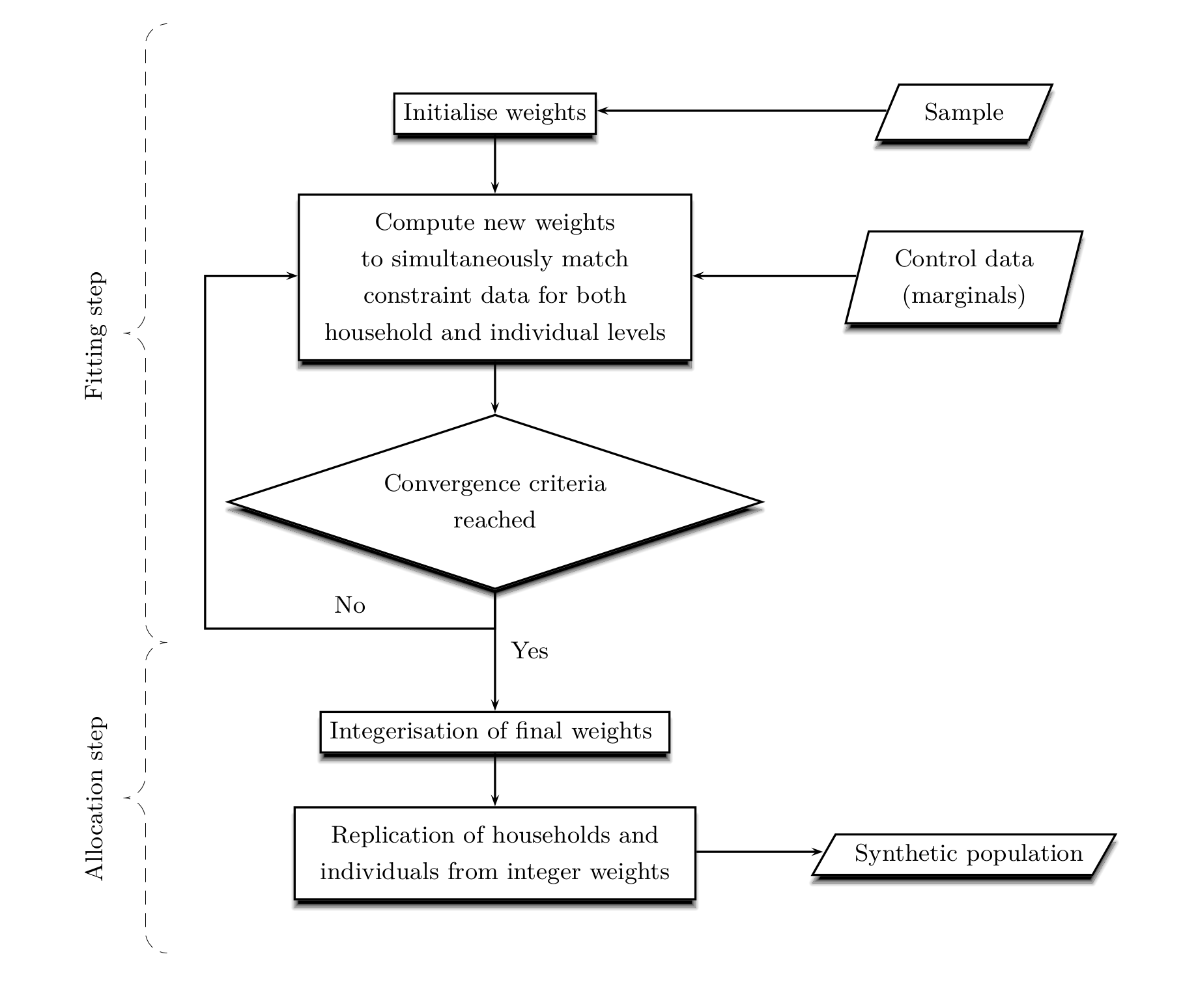
This category of methods is the most widely used to generate synthetic populations. A synthetic population is produced according to a two-step procedure: fitting and allocation. The fitting step involves assigning positive weights to the individuals and households contained in the sample with the resulting weights typically being non-integers. During the allocation step, these non-integer weights are converted into integer weights in order to replicate individuals and households.
SR methods are deterministic methods, meaning that depending on the sample studied, the weights obtained during the fitting step never vary. The prerequisite to applying SR methods is to possess both a sample and aggregate data. The underlying assumptions here are twofold: the sample represents the true correlation structure among the attributes (Farooq et al. 2013); and the interactions present in the sample are, to a great extent, preserved for the synthetic agents (Müller & Axhausen 2010). The sample therefore needs to be consistent, representative and composed of at least one observation for each type of individual in the actual population.
One of the commonly used SR techniques is Iterative Proportional Fitting (IPF) (Beckman et al. 1996; Pritchard & Miller 2012), which adjusts a contingency table constructed from the sample so as to match marginal distributions.
In its original formulation, IPF cannot simultaneously estimate both household and individual-level attributes. Some IPF-based algorithms have attempted to address both household and individual attributes (Arentze et al. 2007; Auld & Mohammadian 2010; Guo & Bhat 2007; Pritchard & Miller 2012; Zhu & Ferreira Jr 2014). However, in all these studies, the joint distribution of household and individual-level attributes is fitted either separately or sequentially which fails to guarantee the consistency between these two levels. Another approach consists of a fitting stage using IPF and a simulation stage where individuals are grouped into households with a household allocation procedure using the concept of "spouse matching" and "kids matching" (Rich 2018).
In order to generate a two-layered synthetic population, four main algorithms have been proposed: Iterative Proportional Update (IPU) (Ye et al. 2009), Hierarchical Iterative Proportional Fitting (HIPF) (Müller 2017; Müller & Axhausen 2012), relative entropy minimization (ent) (Lee & Fu 2011), and Generalized Raking (GR) (Deville et al. 1993). In effect, these techniques generate populations of individuals grouped into households by computing household-level weights that satisfy the marginals at both the household and individual levels. Such algorithms will prove to be the most appropriate for the case study presented below, in considering the available input data, and will be presented in greater detail in the third section.
Combinatorial optimization
The second category of approaches falls under to Combinatorial Optimization (CO) techniques. CO based techniques are two-layered since they can directly generate a list of households and individuals (Ma & Srinivasan 2015).
Similar to SR methods, CO requires information on both the sample and marginal level, with the synthetic population being obtained by replicating individuals (without explicitly determining the joint distribution across all controlled attributes). But unlike SR methods, Combinatorial Optimization is a stochastic process. The data requirements for CO methods are less restrictive than those for SR methods (Templ et al. 2017), though on the other hand they do suffer from computational complexity when the population size is large (Lee & Fu 2011). A description of this method has been given by Voas & Williamson (2000) and Templ et al. (2017).
Statistical learning
The third approach available to generate a two-layered synthetic population is Statistical Learning (SL), also known as the simulation-based approach. SL focuses on the joint distribution of all attributes in the sample by directly estimating a probability for each combination, including those not observed in the sample (Sun et al. 2018).
SL methods offer greater flexibility in terms of data requirements and data sources; in general, they display good performance both in treating the lack of heterogeneity problem encountered in SR and CO (Sun et al. 2018) and with small samples (Borysov et al. 2019; Sun et al. 2018). However, a major drawback of SL methods is their inability to satisfy the conditional distributions while satisfying the marginal distributions of all variables simultaneously. During the population synthesis process, when marginals are available, it is indeed necessary to precisely match the observed marginal distributions with the population generated at the zonal level. Some of the two-layered SL-based algorithms derived for synthetic population generation include: the hierarchical Chain Monte Carlo method (hMCMC) (Farooq et al. 2013), the Bayesian Networks-based method (Sun & Erath 2015; Zhang et al. 2019), hierarchical mixture modeling (HM) (Sun et al. 2018), and deep generative modeling based on a Variational Autoencoder (VAE)(Borysov et al. 2019).@ye2019consistent proposed a tensor decomposition method to guarantee the consistency between three levels of constraints: individual, household and enterprise.
A comparison of methods
Two-layered SR methods (IPU, HIPF, ent and GR) can generate high-quality two-layered synthetic populations that closely represent the actual population. Nonetheless, such techniques require a major preprocessing effort and are very stringent in terms of data needs. In fact, they require a representative sample and aggregate statistics at both the individual and household levels (Chapuis & Taillandier 2019). CO methods are less restrictive on data quality than SR methods for generating a two-layered synthetic population, yet they cannot always guarantee the optimal solution with respect to matching marginals and moreover require too much computing time. This CO category is better suited for generating small synthetic populations. SL methods are able to produce consistent results even for small sample sizes and generate a synthetic population from sample data only when necessary. On the other hand, SL methods make it impossible to satisfy marginal distributions of variables, which constitutes a major drawback when these marginals are available. In some configurations, combining SR and SL methods could be the most relevant option to have an accurate synthetic population satisfying marginal distributions. For example, combining a Variational Autoencoder model with IPF and quota-based random sampling (Borysov et al. 2019) or Bayesian Networks with Generalized Raking techniques (Sun & Erath 2015).
The aim of this paper is to generate two-layered synthetic populations using French census data. The particularity of this dataset is the availability of a representative sample at the municipality level. The sample size is roughly 30% of the total municipal population; furthermore, aggregate statistics for both individual and household attributes are available which ensures data consistency. The data requirements for using SR methods in order to generate a synthetic population of individuals and households are therefore being met. Hence, SR methods are best suited since neither CO nor SL methods will not provide any advantage over SR. CO methods will in fact limit the population size potentially generated while SL methods prevent fitting to the marginals. The SR methods adopted to generate the synthetic population will be detailed in the next section.
Synthetic Population Generation Methodology
The synthetic population is generated using a two-step procedure: 1- fitting, and 2- allocation (see Figure 1). In the first subsection, the four two-layered SR methods (Iterative Proportional Update (IPU), Hierarchical Iterative Proportional Fitting (HIPF), relative entropy minimization (ent) and Generalized Raking (GR)) available for use during the first step are presented. The second subsection then describes the two methods (proportional probabilities approach and TRS method) that convert non-integer weights resulting from the fitting step into integer weights in order to replicate individuals and households.
The fitting step
The objective of this step is to find the vector of household weights: \(W=(w_{h})\), where \({h=1\ldots n^s_{h}}\). \(n^s_{h}\) is the number of households in the sample and \(w_{h}\) is a positive real measuring the importance of the corresponding household. This weight will be used in the allocation step to repeat or draw its corresponding household. Marginals are modeled as constraints on the weights vector.
We propose formulating this problem within the framework of the regularization of ill-posed inverse problems1 in order to clarify the comparison among the various algorithms. From this point of view, the objective here is to find \(W\) that satisfies the marginal constraints, i.e.:
| \[\begin{gathered} O^H\cdot W=M^{H}\\ O^I\cdot W=M^{I}\\ W\geq 0 \end{gathered} \] | \[(1)\] |
This problem is ill-posed inasmuch as there are more variables than constraints (\(n_{m}= n_{mh}+ n_{mi}< n^s_{h}\)). The constraints are often inconsistent with one another. The solution therefore must be regularized. An intuitive regularization consists of seeking a solution that is not too far removed from the sample, i.e. the vector solution \(\hat{W}\) is not too distant from the vector of the prior weights, \(W^{prior}\), which models the sample. The following optimization problem serves to translate this idea.
| \[\hat{W} = \operatorname*{arg\,min}_{\substack{ W\geq 0 \\ O^H\cdot W\simeq M^{H}\\ O^I\cdot W\simeq M^{I}}} \mathop{\mathrm{dist}}(W, W^{prior}) \] | \[(2)\] |
The Statistical Reconstruction (SR) methods described in this paper, i.e. Iterative Proportional Update (IPU), Hierarchical Iterative Proportional Fitting (HIPF), Relative Entropy Minimization (ent) and Generalized Raking (GR), can all be interpreted within this common framework: these methods are in fact different views of the regularized Problem 2 of ill-posed Problem 1. For ent and GR, the minimization is explicit though the distance measurement differs. For IPU and HIPF, the minimization is implicit.
- Iterative Proportional Update offers a geometric point of view of Problem 2. The IPU method starts from the sample, with initial weights being uniform. This vector is projected onto the hyperplane corresponding to household constraints before being projected onto a second hyperplane corresponding to the constraints on individuals. The process is iterative in support of the purpose of this algorithm to find a solution which is not too far removed from the initial sample and consistent with the constraints. It can be interpreted as a heuristic solution of Problem 2. IPU has been proven to have some limitations when generating a synthetic population at both individual and household levels. In particular, Ye et al. (2020) have shown that theoretically, IPU is unable to converge to an optimal population distribution that simultaneously satisfies the constraints from individual and household levels. The authors have proposed an extension of IPU in order to address IPU failures. However, in our use case, IPU generates suitable solutions because the sample is large.
- Hierarchical Iterative Proportional Fitting presents a dual view of Problem 2: it minimizes the distance to both constraint types on households and individuals, starting from uniform initial weights. The weights are modified as little as possible while optimizing the distance to the constraints.
- Relative Entropy Minimization conveys a probabilistic point of view of Problem 2. The objective is to determine a probability, \(\mathop{\mathrm{p}}_{h}\), associated with each household that can be interpreted as the weight, \(w_{h}\), divided by the number of households in the target population, \(n_{h}\). The solution must satisfy the marginal constraints and minimize the relative entropy to a prior, nearly uniform probability. By dividing in Problem 2, the weights vectors by the size of the target population and then by replacing the distance operator \(\mathop{\mathrm{dist}}(\mathop{\mathrm{p}}_{h},\mathop{\mathrm{p}}_{h}^{prior})\) by \(\mathop{\mathrm{p}}_{h}\log(\frac{\mathop{\mathrm{p}}_{h}}{\mathop{\mathrm{p}}_{h}^{prior}})\), the entropy formulation can be derived.
- Generalized Raking provides an optimization point of view of Problem 2. It proposes solving this problem by setting up the Lagrangian.
After this more comprehensive introduction of the framework for treating inverse problems, the various methods will now be presented in greater depth.
Iterative proportional update
The Iterative Proportional Update (IPU), developed by Ye et al. (2009), is an iterative heuristic algorithm that simultaneously controls individual and household-level marginals during the fitting procedure. The corresponding mathematical optimization problem can be formulated with the following objective function (Ye et al. 2009):
| \[\min_{\substack{w_{h}}} \quad\sum_{j}\left[\left(\sum_{h}o_{j,h}w_{h}- m_{j}\right)/m_{j}\right]^2\quad\] | \[(3)\] |
The objective function measures the inconsistency between the weighted sample and the given constraints. At the first iteration, all households have a weight of one. IPU typically starts by adjusting weights to satisfy household constraints first, then updating them to satisfy individual constraints. At each iteration, a statistical measurement \(\delta\) provides a goodness-of-fit result; it is the average of the absolute value of the relative difference between the weighted sum and the constraints, i.e.:
| \[\delta= \frac{ \sum_{j}\left[\left|\left(\sum_{h}o_{j,h}w_{h}- m_{j}\right)\right|/m_{j}\right]}{n_{m}}\] | \[(4)\] |
The gain in fit between two consecutive iterations is then calculated (\(\Delta=\lvert \delta_a-\delta_b \rvert\)). The entire process is continued until the gain in fit is negligible or below a preset tolerance level. This tolerance level serves as the convergence criterion for terminating the algorithm (Ye et al. 2009).
Hierarchical iterative proportional fitting
The HIPF algorithm (Müller 2017; Müller & Axhausen 2011) converts the household-level weights into individual-level weights and vice versa. It also proceeds in iterations and the procedure can be defined as follows (Müller & Axhausen 2011):
- \(k \leftarrow 0\)
- \(w_{h}^{0} \leftarrow 1\) for all \(\quad h \in S\)
repeat - \(w_{h}^{(k+1)} \leftarrow\text{FIT} ( w_{h}^{(k)},m^{h}_a,m^{h}_b,...)\) for all \(\quad h \in S\)
- \(w_{hi}^{(k+2)} \leftarrow w_{h}^{(k+1)} \quad\) for all\(\quad i \in S \quad\) for all \(\quad i \in I(h)\)
- \(w_{hi}^{(k+3)} \leftarrow \text{FIT} ( w_{hi}^{(k+2)} ,m^{i}_\alpha,m^{i}_\beta,...)\quad\) for all \(\quad h \in S\) for all \(\quad i \in I(h)\)
- \(w_{h}^{(k+4)} \leftarrow \frac{1}{n_{mi}(h)}\sum_{i\in I(h)}w_{hi}^{(k+3)} \quad\) for all \(\quad h \in S\)
- estimate \(w_{h}^{(k+5)} \quad \text{from}\quad w_{h}^{(k+4)} \quad\) by adjusting the individuals-per-household
ratio using the relative entropy minimizing. - \(k\leftarrow k+5\)
until convergence
return \(w_{h}^{(k)}\)
In the above algorithm, \(h\) denotes a household, \(i\) an individual, \(k\) the iteration number, \(w_{h}^{(k)}\) the weight attributed to the h\(^{th}\) household, \(w_{hi}^{(k)}\) the weight attributed to the i\(^{th}\) individual in household \(h\), \(m^{h}_a\) and \(m^{h}_b\) are household-level control totals, and \(m^{i}_\alpha\) and \(m^{i}_\beta\) individual-level control totals. Moreover, \(S=\{1\ldots n^s_{h}\}\) with \(n^s_{h}\) being the number of households in the sample. \(P(h) = \{1 \ldots n_{mi}(h) \}\), whereby \(n_{mi}(h)\) is the number of individuals in household \(h\).
At the first iteration, all households have a weight of one. For all households, weights are computed to fit household-level control totals and converted to individual-level weights. These weights are then used as initial values to estimate new individual-level weights to fit the individual-level control totals. The next step (Step 5) is to convert these new individual-level weights to household-level weights by considering that the weight of each household equals the average of the sum of the weights of the individuals in that household.
The sixth step consists of recomputing new household weights (\(w_{h}^{(k+5)}\)) by minimizing the relative entropy from weights obtained in Step 5 (\(w_{h}^{(k+4)}\)) to these latest weights, as defined below:
| \[\text{D}\left(w_{h}^{(k+5)} || w_{h}^{(k+4)}\right)=\sum_h w_{h}^{(k+5)}\ln \frac{w_{h}^{(k+5)}}{w_{h}^{(k+4)}} \] | \[(5)\] |
| \[\sum_{h=1}^{n^s_{h}} w_{h}^{(k+5)}= n_{h}\] | \[(6)\] |
| \[\sum_{h=1}^{n^s_{h}} \sum_{i=1}^{n_{mi}(h)} w_{hi}^{(k+5)} = n \] | \[(7)\] |
Entropy minimization
A mathematical formulation, using the relative entropy minimization function as the objective function, to generate synthetic data was proposed by Bar-Gera et al. (2009) and Lee & Fu (2011). According to this approach, both household and individual-level characteristics are contained in the constraints. The entropy optimization (ent) method described in this section closely follows that of Lee & Fu (2011).
Let’s consider the following notations: \(n_{h}\) and \(n\) are respectively the total number of households and total population in the research area; \(n_v\) and \(n_u\) respectively the number of household-level and individual-level characteristics (factors); \(\alpha\) and \(\beta\) are two subsets of respectively \(\{1, 2,\dots, n_v\}\) and \(\{1, 2,\dots, n_u\}\) (\(\alpha\) and \(\beta\) will be used to model the marginals); \(x^{h}_{v}\) represents one household-level characteristic and \(x^{i}_{u}\) represents one individual-level characteristic; \(x^{h}_{\alpha}\) represents the household-level characteristics associated with subset \(\alpha\) (\(x^{h}_{\alpha}\) = \((x^{h}_{v})_{v\in \alpha}\)), while \(x^{i}_{\beta}\) represents individual-level characteristics associated with \(\beta\) (\(x^{i}_{\beta}\) = \((x^{i}_{u})_{u\in\beta}\)).
Furthermore, let’s consider:
- \(nx^{i}_{u}\) is the number of people in household \(h\) with person-level characteristic \(x^{i}_{u}\) where \(nx^{i}_{u}\in \mathbb{N}\) and where \(u=1,2,\dots,n_u\); \(nx^{i}\), is the vector of possible number of people in a household with a given individual-level characteristic and \(nx^{i}\) equals \(\{nx^{i}_1,\dots,nx^{i}_u,\dots,nx^{i}_{n_u}\}\);
- \(h_{v}\) denotes one possible value of \(x^{h}_{v}\), where \(h_{v}\in \Omega_v\), and \(\Omega_v\) is a finite domain of values of \(x^{h}_{v}\), where \(v\) is equal to \(1,2,\dots, n_v\); \(h_{\alpha}\) denotes one possible value of \(x^{h}_{\alpha}\), where \(h_{\alpha} \in \prod_{v\in \alpha} \Omega_v\); and \(h\) is the vector of all possible values of \(x^{h}\);
- \(nx^{i}_{\beta}\) is the number of people in household h with person-level characteristics \(x^{i}_{\beta}\), where \(nx^{i}_{\beta} \in \prod_{u \in \beta}\mathbb{N}\).
Using the above notations, \(\widetilde{\mathop{\mathrm{p}}}_{\alpha}(h_{\alpha})\), \(\widetilde{E}_{\beta}(nx^{i}_{\beta})\), and \(\mathop{\mathrm{p}}_{[h,nx^{i}]}\) are defined as follows:
- \(\widetilde{\mathop{\mathrm{p}}}_{\alpha}(h_{\alpha})\) = joint distribution across household-level characteristics \(x_{\boldsymbol{\alpha}}\), where \(\widetilde{\mathop{\mathrm{p}}}_{\alpha}(h_{\alpha})\) = \(m^{h}(h_{\boldsymbol{\alpha}})/n_{h}\) and where \(m^{h}(h_{\boldsymbol{\alpha}})\) is the aggregate summary count across household-level characteristic \(x^{h}_{\alpha}\);
- \(\widetilde{E}_{\beta}(nx^{i}_{\beta})\) = expected number of people in one household across person-level characteristics \(x^{i}_{\beta}\), where \(\widetilde{E}_{\beta}(nx^{i}_{\beta}))\) = \(m^{i}(x^{i}_{\beta})/n_{h}\); and \(m^{i}(x^{i}_{\beta})\) is the count of person-level characteristics \(x^{i}_{\beta}\), with \(\sum_{\beta} m^{i}(x^{i}_{\beta})\) = \(n\);
- \(\mathop{\mathrm{p}}_{[h,nx^{i}]}\) = multiway proportion of households in the research area with household-level characteristics \(h\) = \(\{h_1,\dots, h_v,\dots, h_{n_v} \}\) and number of individuals with person-level characteristics \(x^{i}\), \(nx^{i}= \{nx^{i}_1,\dots ,nx^{i}_u,\dots, nx^{i}_{n_u}\}\) and \(u=1,2,\dots,n_u\).
- \(\mathop{\mathrm{p}}_{[h,nx^{i}]}^{prior}\)= prior \(\mathop{\mathrm{p}}_{[h,nx^{i}]}\), easily computed from the disaggregated sample.
The objective is to minimize the relative entropy between \(\mathop{\mathrm{p}}_{[h,nx^{i}]}\) and \(\mathop{\mathrm{p}}_{[h,nx^{i}]}^{prior}\) (i.e. the estimation of \(\mathop{\mathrm{p}}_{[h,nx^{i}]}\) must be discriminated from \(\mathop{\mathrm{p}}_{[h,nx^{i}]}^{prior}\) with a minimum difference).3
This objective function can be written as follows:
| \[\min_{\substack{\mathop{\mathrm{p}}_{[h,nx^{i}]}}} \quad \text{D}({\mathrm{p}}_{[h,nx^{i}]}|| {\mathrm{p}}_{[h,nx^{i}]}^{prior})=\sum_{h,nx^{i}} {\mathrm{p}}_{[h,nx^{i}]}\ln\left(\frac{{\mathrm{p}}_{[h,nx^{i}]}}{\mathop{\mathrm{p}}_{[h,nx^{i}]}^{prior}}\right) \] | \[(8)\] |
| \[\sum_{\{h, nx^{i}| v \notin \alpha\}}\mathop{\mathrm{p}}_{[h,nx^{i}]}=\widetilde{\mathop{\mathrm{p}}}_{\alpha}(h_{\alpha}) \quad\forall h_v \in \Omega_v,\quad v=1,2,...,n_v,\quad h_\alpha \in \prod_{v\in \alpha} \Omega_v \] | \[(9)\] |
| \[\sum_{ nx^{i}_\beta} nx^{i}_\beta \left( \sum_{\{h, nx^{i}| u\notin \beta\}}\mathop{\mathrm{p}}_{[h,nx^{i}]}\right)=\widetilde{E}_{\beta}(nx^{i}_{\beta})\quad \forall nx^{i}_{u}\in \mathbb{N},\quad \quad u=1,2,...,n_u, \quad nx^{i}_{\beta} \in \prod_{u \in \beta} \mathbb{N} \] | \[(10)\] |
| \[\mathop{\mathrm{p}}_{[h,nx^{i}]}\geq0 \quad \sum_{h, nx^{i}} \mathop{\mathrm{p}}_{[h,nx^{i}]}=1 \] | \[(11)\] |
This formulation is an implementation of Problem 2, in considering probability \(\mathop{\mathrm{p}}_{[h,nx^{i}]}\) instead of weight \(w_{h}\), by inputting in Equation 9 and 10 the constraints on households and on individuals and by instantiating the distance measurement \(\mathop{\mathrm{dist}}\left(\mathop{\mathrm{p}}_{h},\mathop{\mathrm{p}}_{h}^{prior}\right)\) with \(\mathop{\mathrm{p}}_{h}\log\left(\frac{\mathop{\mathrm{p}}_{h}}{\mathop{\mathrm{p}}_{h}^{prior}}\right)\).
Generalized raking
The Generalized Raking (GR) techniques were developed by Deville et al. (1993) to generate a synthetic population of both individuals and households. These techniques allow adjusting sampling weights in order to match known population totals. The problem formulation aligns with that of Deville et al. (1993) and Müller (2017).
Let’s now consider a finite population U = \(\{1,\dots,h,\dots, n_{h}\}\) with a response variable \(y_h \in \mathbb{R}\). A sample \(s\) of size \(n^s_{h}\) is drawn from U with a given sampling design such that the inclusion probabilities \(\mathop{\mathrm{p}}_{h,x}^{inclusion}= P(x \in s)\) are known. Let \(y_h\) be the value of a variable of interest \(y\) , for the h\(^{th}\) population element. The objective then is to estimate the finite population total \(t_y= \sum_{h\in U} y_h\). An unbiased commonly used estimator of \(y\) is the Horvitz–Thompson estimator:
| \[{\hat{y}} = \sum_{h\in s}\frac{1}{\mathop{\mathrm{p}}_{h,x}^{inclusion}} y_h = \sum_{h\in s} w_{h}^{prior}y_h \] | \[(12)\] |
| \[\min_{\substack{ w_{h}}} \sum_{h \in s} w_{h}^{prior}G (w_{h}/w_{h}^{prior}) \] | \[(13)\] |
| \[\sum_{h \in s} w_{h}\boldsymbol{X}_h = M \] | \[(14)\] |
This problem can now be solved by introducing a vector of Lagrange multipliers as demonstrated in Deville et al. (1993).
This formulation is an implementation of Problem 2, by instantiating the distance measurement \(\mathop{\mathrm{dist}}\left( w_{h},w_{h}^{prior}\right)\) with \(w_{h}^{prior}G(\frac{w_{h}}{w_{h}^{prior}})\) and by identifying \(\boldsymbol{X}_h\) with the occurrence matrix \(O\).
Generation process comparison across the four methods
Iterative Proportional Update (IPU), Hierarchical Iterative Proportional Fitting (HIPF) and relative entropy minimization (ent) all generate populations of individuals grouped into households by computing household-level weights that satisfy the marginals at both the household and individual levels. The HIPF algorithm constantly switches between household and individual domains, in employing an entropy-optimizing adjustment step (Müller & Axhausen 2011). With the IPU and ent algorithms, weights are adjusted to satisfy household-level constraints first and then updated to satisfy individual-level constraints. The difference between IPU and ent lies in the procedure applied to adjust weights for a given individual-level control: if a household contains two or more individuals of the same category, ent reweights this household more heavily than a household with just one individual from this category, while IPU makes no distinction (Müller 2017). The Generalized Raking method directly adjusts weights to satisfy both individual and household-level constraints.
The allocation step
All the methods described above generate fractional weights of households and individuals, making the results difficult to analyse. To construct the final population, we thus need to integerize these weights. The integerization process refers to converting these fractional weights into integer weights. To achieve this, two probabilistic methods are used: the proportional probabilities approach, and the truncate replicate sample (TRS) method. According to Lovelace et al. (2015), both of them outperform deterministic methods (simple rounding, threshold approach) in terms of final population counts and accuracy.
The proportional probabilities approach
The proportional probabilities (PP) approach considers fractional weights as probabilities (Joubert 2018; Lovelace et al. 2015). For example, the probability \(p_h\) of a given household lies in the final synthetic population is thus given by: \(p_h=w_{h}/\sum w_{h}\). The higher the fractional weight, the more likely an individual/household lies in the final population. As a result, an individual with a very high weight may be replicated several times, while one with a very low weight might not be included in the final synthetic population.
The TRS approach
The TRS approach (Lovelace & Ballas 2013) combines deterministic and probabilistic sampling in order to generate integer weights according to a three-step process: truncation, replication, and sampling.
- The truncation step yields integer values by removing all information to the right of the decimal point. The decimal remainders (between 0 and 1) are then kept. As an illustration, a household with a weight of 4.65 will have a truncated value of 4. Its decimal remainder is 0.65.
- During the second step, individuals/households are replicated depending on their integer weights obtained during the truncation step. Only truncated weights greater than 0 are replicated. For example, the household with a weight of 4.65 will be replicated 4 times. Another household with a weight of 0.99 would not be replicated in this step (its truncated value is 0). When performing truncation and replication, no chance of oversampling exists (i.e. the sum of all integer weights will always be less than the population size).
- During the last step, only the decimal weight remainders are included in applying a weighted random sampling without replacement. The rest of the individuals/households are selected from the entire sample, with selection probabilities set equal to the decimal weight remainders. In our example, the household with the starting weight of 4.65 will have a 0.65 probability of being chosen again, while the other household will have a 0.99 probability.
Case Study
The performance of the various methods described above will now be assessed using data drawn from the French census. This dataset has been collected by the French National Institute of Statistics and Economic Studies (INSEE). Since 2004, this census has covered all municipalities and is valid over a five-year period. By compiling successive five-year surveys, an array of population statistics could be obtained. To build a more robust database, the collected data were then adjusted to a single reference date, thus ensuring that all municipalities were being treated equally. This reference date was set on January 1\(^{st}\) of the median five-year survey period.4
The data provided by INSEE are available in two distinct forms: a sample of individuals and households, and control variables, both at the level of an IRIS (acronym for "aggregated units for statistical information"), which represents the basic unit for dissemination of intra-municipal data. Municipalities with over 10,000 inhabitants, and a large proportion of those with 5,000 to 10,000 population, are divided into several IRIS units and, by extension, all municipalities not divided into IRIS units constitute IRIS units in themselves.
We are specifically using census data from the Nantes Urban Area5 (NUA) from 2015 (these data were collected from 2013 to 2017). The total population of the NUA was approximately 949,000 individuals, residing in 418,000 households within 307 IRIS or equivalent units. The sample included 287,000 individuals and 136,000 households. Each observation in the sample represents a unique individual with his or her personal characteristics, as well as the household and main residence characteristics. Table 1 describes the attributes used in the generation process.
Descriptive statistics
Table 1 describes the variables collected for all 307 IRIS included in the sample. For our analysis, we considered 5 variables at the individual level and 4 variables at the household level. An IRIS contains on average of 1,363.3 households (\(\pm 631.3\)) and 3,092.2 individuals (\(\pm 1,334.6\)); the samples contain on average 32.30% of households (\(\pm 11.36\)) and 30.87% of individuals (\(\pm 9.96\)) from the actual population.
| Level | Variable | Definition [number of categories] | Categories |
| Household | Fam | Family composition [5] | Single member; The nuclear family is a couple without children; The nuclear family is a couple with children; The nuclear family is a single-parent family; Other composition |
| ProfRP | Profession of the reference person [7] | Farmers, tradespeople; Executive; Intermediate occupations; Clerical support workers; Lower-skilled technical occupations; Retiree; Unemployed | |
| Size | Household size [2] | One person; Two persons or more | |
| Cars | Number of cars [3] | No car; One; Two or more | |
| Individual | Age | Age [12] | 0-2; 3-5; 6-10; 11-14; 15-17; 18-24; 25-29; 30-39; 40-54; 55-64; 65-79; 80/+ |
| Sex | Gender [2] | Female; Male | |
| Relate | Relationship to the household reference person [2] | Household reference person; Other household member | |
| Prof | Profession [7] | Farmers, tradespeople; Executive; Intermediate occupations; Clerical support workers; Lower-skilled technical occupations; Retiree; Unemployed | |
| Wstat | Work status [7] | In fixed-term employment; Permanent employment; Self-employed; Unpaid apprenticeships for those 15 or older; Unemployed; Under 15 years old; Other non-active persons | |
| Wtime | Working time [3] | Full-time worker; Part-time worker; Not applicable |
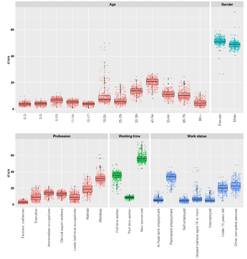
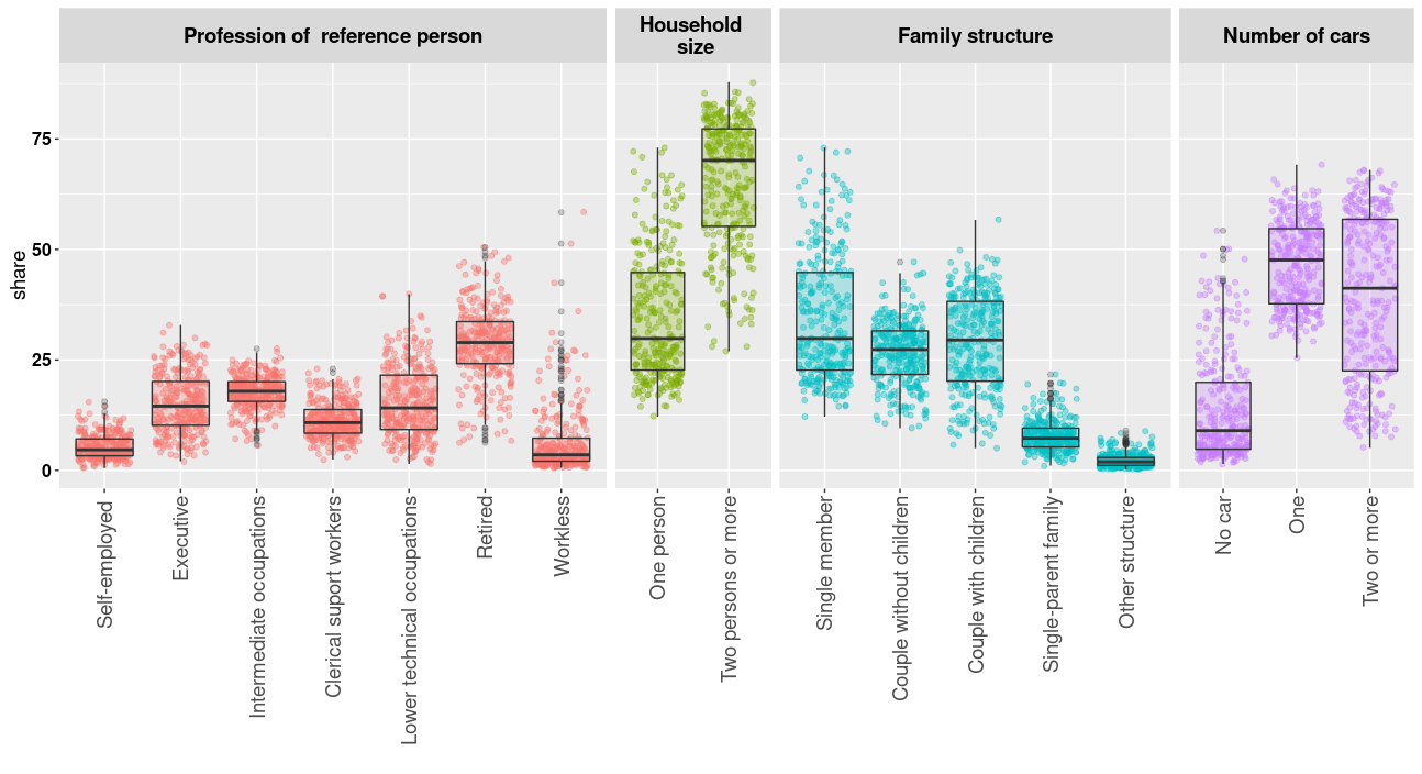
Figure 2 and 3 display the distributions of the shares of the various categories of individual-level and household-level variables within the 307 IRIS. For most of these distributions, a fairly large variability can be observed.
Validation
The next section will compare the four previously described approaches to generating a synthetic population of households and individuals: IPU, HIPF, ent and Generalized Raking.6 For each of these, we have used the proportional probabilities (PP) and truncate replicate sample (TRS) methods to integerize the weights. We have thus evaluated not only the performance of the four generation approaches but also that of the two integerization techniques.
Two main aspects can be considered regarding an evaluation of the accuracy of a synthetic population: internal validation and external validation. Internal validation consists of comparing the variables of the synthetic population with the marginals in order to test the reliability of the generated data (e.g. does the estimated distribution of family composition correspond to distribution given by the census data?). In other words, an internal validation tests the ability of the population to fit with aggregate data. A validation is external if the estimated variables of the synthetic population are compared with another data source not used in the estimation process. Our case study does not feature a data source external to the French census at the IRIS level. Hence, we have solely focused on the internal validation.
According to the literature, internal validation can be carried out on either variables (marginals are compared with corresponding ones in the synthetic population), cells or the entire synthetic population. Many quantitative methods are available for internal validation (Lovelace et al. 2015; Timmins et al. 2016). The following performance metrics have been considered herein:
- The coefficient of determination \(R^2\) is the square of the Pearson correlation; it is a quantitative indicator that varies between 0 and 1 and moreover reveals how closely the simulated values fit the census data. An \(R^2\) value of 1 denotes a perfect fit, while an \(R^2\) value close to zero suggests no correspondence between constraints and simulated values (Lovelace et al. 2015).
- Total absolute error (TAE) and the standardized absolute error (SAE). TAE is the sum of the difference between simulated values and the marginals and SAE is TAE divided by the total population.
- Standardized Root Mean Squared Error (SRMSE). This indicator focuses on error dispersion and is used to evaluate the goodness of fit between the estimated synthetic population and the marginals; it is the one of the most common indicators used (Lee & Fu 2011; Lovelace et al. 2015; Saadi et al. 2016; Sun & Erath 2015). A zero value indicates a perfect match between census data and synthetic population, while a high SRMSE value suggests a poor fit.
- The Bland-Altman method. Widely employed in healthcare studies to compare two measurements of the same variable, this graphical method can also be used to complement the other indicators (Timmins et al. 2016). The Bland-Altman method consists of plotting of the difference between simulated and census counts versus the averages of the two counts.
Results and Discussion
This section presents the results of the internal validation procedure. The four SR algorithms have been implemented in the open-source MultiLevelIPF7 extension to the R statistical software package.8 A synthetic population has been generated for each IRIS of the NUA.
Internal validation with \(R^2\), TAE, SAE and SRMSE
The validation results show that all the proposed methods produce synthetic populations that are representative of the actual population, yet some methods prove to be more efficient. The first indicator, \(R^2\), revealed that even though all methods tested performed well, the TRS integerization method yielded better results than the proportional probabilities method. Moreover, the results of the Generalized Raking method results were less accurate compared than the other three generation methods. A more detailed description of the \(R^2\) results follows:
- HIPF or IPU combined with TRS (HIPF+TRS or IPU+TRS) yields coefficients above 0.99 for all individual and household-level variables;
- HIPF or IPU combined with the proportional probabilities method (HIPF+PP or IPU+PP) and entropy minimization combined with either the TRS or proportional probabilities method (ent+TRS or ent+PP) yield coefficients greater than or equal to 0.98 for all individual and household-level variables;
- GR combined with either TRS or proportional probabilities method (GR+TRS or GR+PP) yield coefficients greater than or equal to 0.91 for all individual and household-level variables.
The \(R^2\) validation method merely provides an indication of fit and is influenced by outliers. A further analysis based on three other indicators (TAE, SAE and SRMSE), is therefore displayed in Table 2. These results confirm that all methods are globally efficient, but entropy minimization and HIPF do outperform the others.
| Individual-level | Household-level | |||||
| Method | TAE | SAE (%) | SRMSE | TAE | SAE (%) | SRMSE |
| IPU+TRS | 87,046 | 1.53 | 0.0024 | 17,082 | 1.02 | 0.0012 |
| IPU+PP | 188,191 | 3.30 | 0.0032 | 56,529 | 3.3 | 0.0027 |
| HIPF+TRS | 53,436 | 0.94 | 0.0013 | 14,134 | 0.84 | 0.0007 |
| HIPF+PP | 176,612 | 3.10 | 0.0027 | 54,564 | 3.26 | 0.0025 |
| ent+TRS | 50,412 | 0.88 | 0.0008 | 16,621 | 0.99 | 0.0009 |
| ent+PP | 168,567 | 2.96 | 0.0024 | 55,830 | 3.33 | 0.0026 |
| GR+TRS | 252,621 | 4.43 | 0.0090 | 71,778 | 4.28 | 0.0098 |
| GR+PP | 337,630 | 5.93 | 0.0093 | 108,368 | 6.47 | 0.0128 |
Based on Table 2, the method can be ranked in the following order from most to least accurate:
- entropy minimization, HIPF, IPU and GR for the individual level;
- HIPF, entropy minimization, IPU and GR for the household level;
- TRS and proportional probabilities.
According to all the validation indicators considered (\(R^2\), TAE, SAE and SRMSE), it can be concluded as regards the generation methods, slight differences exist between entropy minimization and HIPF. Moreover, these two methods outperform IPU and GR. For the integerization methods, the TRS approach outperforms the proportional probabilities approach. HIPF and entropy minimization combined with TRS therefore provide the best possible approximation of the actual population.
IRIS-level analysis
In addition to the global analysis given above, a local analysis, IRIS by IRIS, has been conducted in order to identify the zones with the highest errors (i.e. IRIS with the highest SAE values). For each method tested, whether at the individual or household level, three IRIS always stood out. Table ¿tbl:bad_iris? presents the values for the two best methods.
| Individual-level | Household-level | ||
| Method | Iris Id | SAE (%) | SAE (%) |
| 136 | 35.25 | 6.63 | |
| HIPF+TRS | 237 | 13.71 | 2.82 |
| 162 | 10.08 | 3.09 | |
| 136 | 14.22 | 36.20 | |
| ent+TRS | 237 | 3.71 | 10.37 |
| 62 | 2.40 | 7.51 |
A qualitative analysis of the constraints from these three IRIS underscores their particular characteristics. IRIS 136 and 237 are activity zones with a small number of households and individuals. The population of IRIS 136 (resp. 237) is 359 (resp. 327) households and 964 (resp. 810) individuals. In these two IRIS, 67% (resp. 51%) of households have just one member; also, most of the inhabitants of these IRIS are men (73% (resp. 62%)) and belong to the 18-54 age group. IRIS 162 is a residential area with 1,163 households and 2,133 individuals. However, a significant portion of the territory is occupied by a psychiatric hospital. In this IRIS, 65% of the households are single-member and 65% of the individuals are between 15 and 64 years old. In conclusion, the simulation runs prove to be accurate for all IRIS except a few due to the particular population breakdown of these IRIS.
Bland-Altman approach
A Bland-Altman plot analysis of the data has been performed for comparing the census and simulated values of each IRIS for a given variable. This graphical method studies the mean difference and constructs limits of agreement (Bland & Altman 1999). The X-axis corresponds to the mean of the two values, and the Y-axis is the difference between these two values. The limits of agreement are defined by \(\pm\) 1.96 \(\times\) the standard deviation of the mean difference. Analysis of the plot can help to identify some anomalies such as systematic overestimation or underestimation of census values by a synthetic reconstruction approach (Kalra & others 2017).
Our analysis has been applied to the 400 possible cases (50 categories of variables \(\times\) 8 synthetic reconstruction approaches). The average of the differences (in both real and absolute terms) between simulated and census values by category for each of method has been computed. Figure 4 shows the mean and standard deviation of these mean values for each fitting method. Let us note that the average of the differences between simulated values and census values, expressed in real terms lies close to zero for the HIPF and entropy methods with a rather low standard deviation. The two measurements listed in Figure 4 would seem to confirm the HIPF and entropy methods outperform Generalized Raking and IPU.
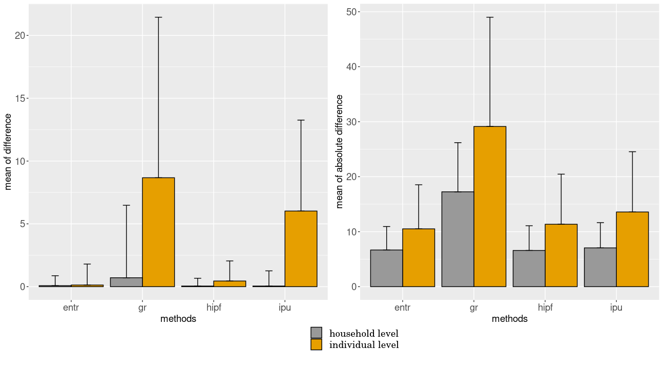
Middle line: mean difference between simulated and census values. Top and bottom lines: limits of agreement.
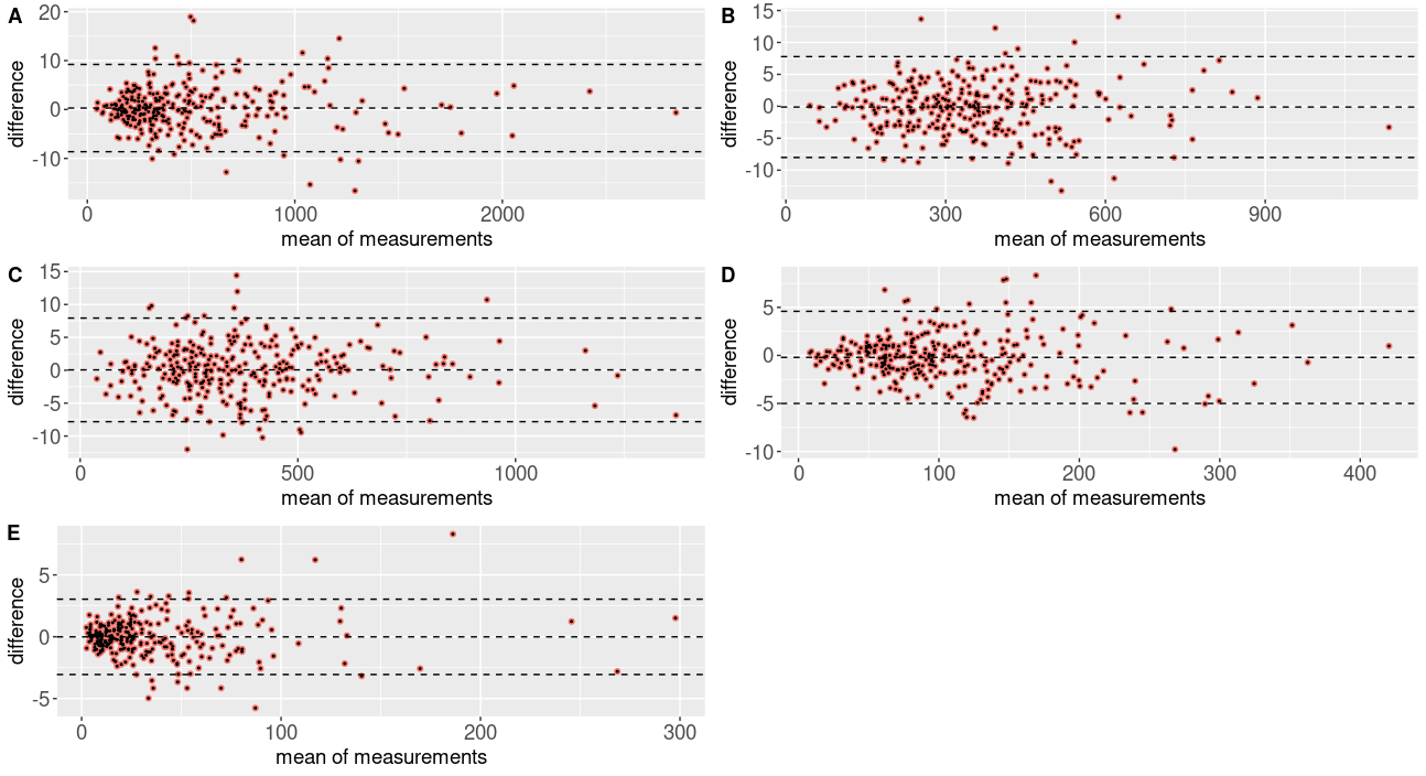
For purposes of illustration, Figure 5 plots Bland-Altman values for the five categories of the household-level variable "Family composition", generated with the HIPF method (in association with TRS allocation approach). The Y-axis shows the difference between the two populations (synthetic and actual), while the X-axis depicts the average of the two values. Depending on the IRIS, the simulated values are in some cases higher and in other cases lower than the census values. The average of the differences (middle line) is close to zero. 95% of the data points lie within the ‘limits of agreement’(top and bottom lines) which indicates that there is agreement between census and simulated values. Depending on the IRIS, the simulated values are in some cases higher and in other cases lower than the census values. This suggests that there is no consistent bias.
Conclusions
This paper has provided a synopsis of the synthetic methods aimed at generating a population of individuals and households. We offered a detailed description of four synthetic reconstruction methods for the fitting step through use of a common framework. These methods are Hierarchical Iterative Proportional Fitting (HIPF), Iterative Proportional Update (IPU), Generalized Raking (GR), and relative entropy minimization (ent). Two integerization methods were also discussed, namely proportional probabilities and truncation replication and sampling (TRS). Next, an evaluation was performed of the most relevant method for generating a two-layered synthetic population. These methods were implemented using the R language. A case study involving the synthesis of agents (418,000 households, 949,000 individuals) from the Nantes Urban Area (western France) was considered, beginning with a sample of 136,000 households, including 287,000 individuals and 15,350 marginals. The synthetic population was generated with four household-level attributes and six individual-level attributes.
Results were evaluated using four indicators: \(R^2\), TAE, SAE, and SRMSE. The validation findings indicate that all methods considered yield good results, i.e. a two-layered synthetic population whose aggregate characteristics lie close to the census marginals. However, some methods output better results than others. For the fitting step, entropy minimization (ent) and Hierarchical Iterative Proportional Fitting (HIPF) prove to be the most efficient methods. For the allocation step, the truncation, replication and sampling (TRS) approach outperforms proportional probabilities.
We believe that the comparison of different statistical reconstruction (SR) algorithms performed in this paper with common notations and a common theoretical framework will facilitate a better dissemination of existing algorithms. This common framework will stimulate the development of new algorithms and position them with respect to existing methods.
The next step is to spatially allocate households or add to the demographic characteristics of households and individuals other socio-economic variables such as income by using other databases, e.g. fiscal database. The mathematical model used in this article inspires our current research to propose data fusion algorithms that enrich the synthetic population.
Appendix: Model Documentation
In this appendix, we describe in five steps the approach used in the paper in a more detailed fashion with an R script. The first step presents the databases used and how to download them. The other steps describe the statistical analyses performed with a toy model. Interested readers can directly contact the authors to get the complete codes.
Step 1: Databases access
The databases used are available under the following links (consulted on 6 November 2020):
- sample data: https://www.insee.fr/fr/statistiques/3625223?sommaire=3558417
- aggregate data from which the control variables are extracted:
- Couple-family-households database: https://www.insee.fr/fr/statistiques/3565598
- Residents’activities database: https://www.insee.fr/fr/statistiques/3627009
- Evolution and structure of the population database: https://www.insee.fr/fr/statistiques/3564100
- Housing database: https://www.insee.fr/fr/statistiques/3564300
Step 2: Data processing
Inputs : downloaded databases
Outputs :
- A R dataframe for the sample.
- For each control variable, we must have a R dataframe. In our case study, we have 10 variables, so we must have 10 R dataframes.
Conditions:
Ensure data consistency.
Each row of the sample dataframe must represent an individual with his or her personal and households characteristics, a unique personnal ID number, a household ID and IRIS ID.
Each row of a control variable dataframe must represent a category with the number of people/households in this category and iris ID.
Step 3 : Fitting step
Use of the four two-layered SR methods (Iterative Proportional Update (IPU), Hierarchical Iterative Proportional Fitting (HIPF), relative entropy minimization (ent) and Generalized Raking (GR)).
Conditions:
-Install MultiLevelIPF package under the following link: devtools::install\(\_\)github("krlmlr/MultiLevelIPF") and then call library(MultiLevelIPF).
Outputs: households weights for each algorithm.
Step 4 : Allocation step
Use of TRS method.
Outputs: synthetic population of households to merge with individuals by household ID.
Step 5 : Validation step
Use of classical performance metrics (\(R^2\), TAE, SRMSE and Bland-Altman) to compare algorithms.
Notes
An abundance of literature exists of this subject ever since the seminal work by Tikhonov & Arsenin (1977).↩︎
In this paper, distance is not intended in its strict mathematical definition.↩︎
In the literature on synthetic population generation, this method is often called cross-entropy minimization; from a strictly mathematical point of view, it is not valid. We have chosen to replace the term cross-entropy by relative entropy, also known as Kullback-Leibler divergence, which is correct and consistent with the notation of D for the measurement of this relative entropy.↩︎
https://www.insee.fr/fr/information/2383265, Consulted on 22 April 2020.↩︎
According to the INSEE Institute, an urban area is a group of adjoining municipalities, without pockets of clear land, encompassing an urban centre (urban unit) providing at least 10 000 jobs, and whose neighboring rural districts or suburban units (urban periphery) account for at least 40% of the employed residents working in the center or in the municipalities attracted by this center.↩︎
For the Generalized Raking approach, four distance functions G can be used: the linear method, the raking ratio method, the logit method, and the truncated linear method. We tested all these functions, but convergence was only achieved for the logit method.↩︎
https://github.com/krlmlr/MultiLevelIPF, Consulted on 24 April 2020↩︎
We used a computer of 2 x 2.60GHz CPU cores and 16 GB RAM.↩︎
References
ARENTZE, T., Timmermans, H., & Hofman, F. (2007). Creating synthetic household populations: Problems and approach. Transportation Research Record, 2014(1), 85–91.
AULD, J., & Mohammadian, A. (2010). Efficient methodology for generating synthetic populations with multiple control levels. Transportation Research Record, 2175(1), 138–147.
AVRAM, S., Figari, F., Leventi, C., Levy, H., Navicke, J., Matsaganis, M., Militaru, E., Paulus, A., Rastringina, O., & Sutherland, H. (2013). The distributional effects of fiscal consolidation in nine EU countries. 88th Annual Meeting of the Transportation Research Board, Washington, DC.
BAR-GERA, H., Konduri, K., Sana, B., Ye, X., & Pendyala, R. M. (2009). Estimating survey weights with multiple constraints using entropy optimization methods.
BECKMAN, R. J., Baggerly, K. A., & McKay, M. D. (1996). Creating synthetic baseline populations. Transportation Research Part A: Policy and Practice, 30(6), 415–429.
BLAND, J. M., & Altman, D. G. (1999). Measuring agreement in method comparison studies. Statistical Methods in Medical Research, 8(2), 135–160.
BORYSOV, S. S., Rich, J., & Pereira, F. C. (2019). How to generate micro-agents? A deep generative modeling approach to population synthesis. Transportation Research Part C: Emerging Technologies, 106, 73–97.
CHAPUIS, K., & Taillandier, P. (2019). A brief review of synthetic population generation practices in agent-based social simulation. SSC2019, Social Simulation Conference.
DEVILLE, J. C., Särndal, C. E., & Sautory, O. (1993). Generalized raking procedures in survey sampling. Journal of the American Statistical Association, 88(423), 1013–1020.
EDWARDS, K. L., & Clarke, G. (2013). 'SimObesity: Combinatorial optimisation (deterministic) model.' In R. Tanton & K. Edwards (Eds.), Spatial Microsimulation: A Reference Guide for Users (pp. 69–85). Berlin Heidelberg: Springer.
FAROOQ, B., Bierlaire, M., Hurtubia, R., & Flötteröd, G. (2013). Simulation based population synthesis. Transportation Research Part B: Methodological, 58, 243–263.
GUO, J. Y., & Bhat, C. R. (2007). Population synthesis for microsimulating travel behavior. Transportation Research Record, 2014(1), 92–101.
HÖRL, S., Balac, M., & Axhausen, K. W. (2018). A first look at bridging discrete choice modeling and agent-based microsimulation in MATSim. Procedia Computer Science, 130, 900–907.
JOUBERT, J. W. (2018). Synthetic populations of South African urban areas. Data in Brief, 19, 1012–1020.
KALRA, A., & others. (2017). Decoding the Bland-Altman plot: Basic review. Journal of the Practice of Cardiovascular Sciences, 3(1), 36.
KICKHÖFER, B., & Kern, J. (2015). Pricing local emission exposure of road traffic: An agent-based approach. Transportation Research Part D: Transport and Environment, 37, 14–28.
LEE, D. H., & Fu, Y. (2011). Cross-entropy optimization model for population synthesis in activity-based microsimulation models. Transportation Research Record, 2255(1), 20–27.
LOVELACE, R., & Ballas, D. (2013). “Truncate, replicate, sample”: A method for creating integer weights for spatial microsimulation. Computers, Environment and Urban Systems, 41, 1–11.
LOVELACE, R., Birkin, M., Ballas, D., & Leeuwen, E. van. (2015). Evaluating the performance of iterative proportional fitting for spatial microsimulation: New tests for an established technique. Journal of Artificial Societies and Social Simulation, 18(2), 21: https://www.jasss.org/18/2/21.html.
MA, L., & Srinivasan, S. (2015). Synthetic population generation with multilevel controls: A fitness-based synthesis approach and validations. Computer-Aided Civil and Infrastructure Engineering, 30(2), 135–150.
MÜLLER, K. (2017). A generalized approach to population synthesis.
MÜLLER, K., & Axhausen, K. W. (2010). Population synthesis for microsimulation: State of the art. Arbeitsberichte Verkehrs-und Raumplanung, 638.
MÜLLER, K., & Axhausen, K. W. (2011). Hierarchical IPF: Generating a synthetic population for Switzerland. PhD Thesis, ETH Zurich.
MÜLLER, K., & Axhausen, K. W. (2012). Multi-level fitting algorithms for population synthesis. Arbeitsberichte Verkehrs-und Raumplanung, 821.
MÜNNICH, R., & Schürle, J. (2003). On the simulation of complex universes in the case of applying the German microcensus. DACSEIS Research Paper Series No. 4, University of Tübingen.
O’SULLIVAN, D. (2008). Geographical information science: Agent-based models. Progress in Human Geography, 32(4), 541–550.
PRITCHARD, D. R., & Miller, E. J. (2012). Advances in population synthesis: Fitting many attributes per agent and fitting to household and person margins simultaneously. Transportation, 39(3), 685–704.
RICH, J. (2018). Large-scale spatial population synthesis for Denmark. European Transport Research Review, 10(2), 63.
SUN, L., & Erath, A. (2015). A Bayesian network approach for population synthesis. Transportation Research Part C: Emerging Technologies, 61, 49–62.
SUN, L., Erath, A., & Cai, M. (2018). A hierarchical mixture modeling framework for population synthesis. Transportation Research Part B: Methodological, 114, 199–212.
SUTHERLAND, H., & Figari, F. (2013). EUROMOD: The European Union tax-benefit microsimulation model. International Journal of Microsimulation, 6(1), 4–26.
TEMPL, M., Meindl, B., Kowarik, A., & Dupriez, O. (2017). Simulation of synthetic complex data: The R package simPop. Journal of Statistical Software, 79(10), 1–38.
TIKHONOV, A. N., & Arsenin, V. Y. (1977). Solutions of Ill Posed Problems. New York, NY: V. H. Winston and Sons (Wiley).
TIMMINS, K. A., Edwards, K. L., & others. (2016). Validation of spatial microsimulation models: A proposal to adopt the Bland-Altman method. International Journal of Microsimulation, 9(2), 106–122.
TOMINTZ, M. N., Clarke, G. P., & Rigby, J. E. (2008). The geography of smoking in Leeds: Estimating individual smoking rates and the implications for the location of stop smoking services. Area, 40(3), 341–353.
VOAS, D., & Williamson, P. (2000). An evaluation of the combinatorial optimisation approach to the creation of synthetic microdata. International Journal of Population Geography, 6(5), 349–366.
YAMÉOGO, B. F., Gastineau, P., Hankach, P., & Vandanjon, P. O. (2021). Comparing methods for generating a two-layered synthetic population. Transportation Research Record, 2675(1), 136–147.
YE, P., Tian, B., Lv, Y., Li, Q., & Wang, F.-Y. (2020). On iterative proportional updating: Limitations and improvements for general population synthesis. IEEE Transactions on Cybernetics, 1–10.
YE, X., Konduri, K., Pendyala, R. M., Sana, B., & Waddell, P. (2009). A methodology to match distributions of both household and person attributes in the generation of synthetic populations. 88th Annual Meeting of the Transportation Research Board, Washington, DC.
ZHANG, D., Cao, J., Feygin, S., Tang, D., Shen, Z.-J. M., & Pozdnoukhov, A. (2019). Connected population synthesis for transportation simulation. Transportation Research Part C: Emerging Technologies, 103, 1–16.
ZHU, Y., & Ferreira Jr, J. (2014). Synthetic population generation at disaggregated spatial scales for land use and transportation microsimulation. Transportation Research Record, 2429(1), 168–177.